Employing functional interactions for characterization and detection of sparse complexes from yeast PPI networks

Abstract

Over the last few years, several computational techniques have been devised to recover protein complexes from the protein interaction (PPI) networks of organisms. These techniques model “dense” subnetworks within PPI networks as complexes. However, our comprehensive evaluations revealed that these techniques fail to reconstruct many ‘gold standard’ complexes that are “sparse” in the networks (only $71$ recovered out of $123$ known yeast complexes embedded in a network of $9704$ interactions among $1622$ proteins). In this work, we propose a novel index called Component-Edge (CE) score to quantitatively measure the notion of “complex derivability” from PPI networks. Using this index, we theoretically categorize complexes as “sparse” or “dense” with respect to a given network. We then devise an algorithm SPARC that selectively employs functional interactions to improve the CE scores of predicted complexes, and thereby elevates many of the “sparse” complexes to “dense”. This empowers existing methods to detect these “sparse” complexes. We demonstrate that our approach is effective in reconstructing significantly many complexes missed previously (104 recovered out of the 123 known complexes or $\sim$47% improvement). Availability: http://www.comp.nus.edu.sg/$\sim$leonghw/MCL-CAw/

Sparse complexes; complex prediction; protein interaction networks; functional interactions.

1 Introduction

Stoichiometrically stable complexes are formed by proteins that physically interact to achieve biological functions within the cell. These complexes interact with individual proteins or other complexes to form functional modules and pathways that drive the cellular machinery. Therefore, a faithful reconstruction of the entire set of complexes is essential to not only understand complex formations, but also the higher level organization of the cell.

Recent advances in high-throughput techniques have enabled to catalogue enormous amounts of physical interaction data particularly in organisms such as Saccharomyces cerevisiae (budding yeast). Typically these interactions are arranged in the form of a protein interaction network (or PPI network) and mined for complexes using computational techniques. From a topological perspective, these complexes are typically interpreted as regions in the network where proteins are densely connected to each other than to the rest of the network (Zhang et al., 2008). Accordingly, several computational methods have been proposed that depend primarily on the topologies of PPI networks, and model dense regions as complexes; for a survey, see (Li et al., 2010; Srihari et al., 2010). For example, MCL (Pereira-Leal et al., 2004) simulates a series of random walks (called a flow), the principle being that when the walks reach a dense region, with high probability, they will continue to remain in that region. By repeated iterations of inflation (thickness) and expansion (spread) of the flow, MCL identifies complexes. MCODE (Bader and Hogue, 2003), on the other hand, identifies “seed” proteins in the network using clustering coefficients and greedily expands in the neighborhood of these seeds to build complexes. CMC (Liu et al., 2009) first generates maximal cliques from the network, and then merges highly interconnected cliques to assemble complexes. HACO (Wang et al., 2009) performs agglomerative clustering by generating small clusters and hierarchically merging them into complexes. HACO improves upon the traditional hierarchical agglomerative clustering (HAC) by allowing for overlaps among the generated complexes. Finally, MCL-CAw (Srihari et al., 2010) produces initial clusters using MCL and then refines these clusters by incorporating core-attachment structure to generate complexes.

We performed comprehensive evaluations (Srihari et al., 2010) of these methods, particularly MCL, MCL-CAw, CMC and HACO, on a variety of yeast PPI networks ranging from raw to highly-filtered and under varying levels of natural as well as artificial noise, and found that these methods failed to detect many known complexes catalogued in the MIPS (Mewes et al., 2006) database. For example, MCL missed 65 out of the 123 MIPS complexes present in the Consolidated_3.19 network from Collins et al. (2007). Even the “union” of these methods missed 52 out of the 123 complexes. Since the goal here is to study genome-wide compositions of complexes (the “complexosome”), failure to detect even the known subset of complexes reflects severe limitations in current methods.

1.1 Insights into the topologies of undetected complexes

In order to understand the characteristics of these missed complexes, we “superimposed” yeast complexes taken from the MIPS benchmark (Mewes et al., 2006) onto the high-confidence Consolidated_3.19 yeast PPI network (Collins et al., 2007) (#proteins: 1622, #interactions: 9704, average node degree: 11.187). This “superimposition” involves identifying the proteins of the benchmark complex in the PPI network, and extracting out the subnetwork induced by those proteins. Figure 1 in Supplementary materials shows this “superimposition” visualized using Cytoscape (Shannon et al., 2003).

The immediate observation, which is of course typical to most PPI networks, was that the network comprised of one main large component and multiple disjoint smaller components of sizes 2 to 50. Out of the 123 MIPS complexes containing at least four proteins in the network, 89 were completely embedded in the main component, and the remaining 34 were “scattered” among more than one components. When we ran MCL on this network, it was able to recover only 58 of these 123 complexes. Of the 65 undetected complexes, 27 complexes were the ones that were “scattered”, and 34 complexes, though intact, had very low interaction densities ($<0.50$) in the network. In fact, some of these complexes lacked internal connectivities to an extent that it was impossible for any algorithm to assemble back these disconnected pieces into whole complexes solely based on topological information. For example, the MIPS complex 510.190.110 (CCR4 complex) had seven proteins in the network scattered among four disjoint components. (shown within ellipses in Figure 1 in Supplementary materials). This complex remained disconnected with a low density of 0.1905, and naturally went undetected by all the four algorithms (a few more examples are available from Supplementary materials).

Further, most MIPS complexes being small (sizes $\leq$ 10-15), lacking in just a few proteins or interactions easily rendered many complexes disconnected or with low interaction densities, resulting in them going undetected. All these findings revealed that a potentially strong correlation existed between the “network constitution” of a complex (the number of member proteins in the network and their connectivities) and the possibility of it being detected using existing algorithms.

This work is strongly motivated by the limitations in existing complex detection methods in successfully detecting complexes, and the aforesaid revelations on the topologies of these undetected complexes within PPI networks. The purpose of our work therefore is two-fold: (i) to characterize these undetected complexes, that is, to quantitatively measure their “network constitution”; and (ii) to propose a novel algorithm employing functional interactions to enhance the “derivability” of sparse complexes, which in turn empowers existing methods in detecting these complexes satisfactorily.

2 Methods

We represent our PPI network as $G=(V,E)$, where $V$ is the set of proteins and $E$ is the set of interactions between the proteins. Each interaction $e=(u,v)\in E$ is assigned a weight $0\leq w(u,v)\leq 1$ that reflects the confidence of the interaction, which is usually determined using an affinity weighting scheme (the weight it is set to 1 if no scheme is used). For any $u\in V$, $\mathcal{N}(u)$ refers to the set of neighbors of $u$. Let $\mathcal{B}=\{B_{1},B_{2},...,B_{m}\}$ be the set of benchmark complexes.

We propose the term sparse complexes for the undetected complexes and “very broadly” define them as follows:

Definition 2.1

Sparse complexes: Given a PPI network $G$ and a set of benchmark complexes $\mathcal{B}$ known to be embedded in $G$, the subset $\mathcal{B}^{\prime}\subseteq\mathcal{B}$ of complexes that cannot be satisfactorily detected from $G$ by existing methods are called sparse complexes.

2.1 Indices for complex derivability from PPI networks

We next propose indices that measure the “derivability” of a benchmark complex from a given PPI network. These indices capture whether or not a benchmark complex is derivable from a given PPI network, and if so, to what extent. We propose two kinds of indices here. The first kind defines definitive criteria to categorize a given benchmark complex as derivable or not from the PPI network, and provides derivability bounds on the number of such complexes in the network. The second kind does not strictly categorize the benchmark complex as derivable or not, but instead assigns a derivability score to the complex.

2.1.1 Derivability indices with bounds

To begin with, a naive yet natural way to categorize a benchmark complex as derivable from a PPI network is if it satisfies two criteria: (i) it has sufficient number of proteins in the network; and (ii) it is connected within the network.

We consider a benchmark complex $B_{i}\in\mathcal{B}$ to be $k$-protein-derivable from $G$ if at least $k>0$ of its member proteins are present in $G$. We consider a $k$-protein-derivable complex to be $k$-network-derivable from $G$ if these member proteins form a connected subnetwork within $G$.

Definition 2.2

$k$-protein-derivable complex: A benchmark complex $B_{i}\in\mathcal{B}$ is $k$-protein-derivable from network $G=(V,E)$ if $|B_{i}\cap V|\geq k$, for some $k>0$.

The set of $k$-protein-derivable complexes in $G$ is represented by $D_{P}(\mathcal{B},G,k)$, and the $k$-protein-derivability index of $G$ is $|D_{P}(\mathcal{B},G,k)|$.

Definition 2.3

$k$-network-derivable complex: A benchmark complex $B_{i}\in\mathcal{B}$ is $k$-network-derivable from $G=(V,E)$ if $|B_{i}\cap V|\geq k$ for some $k>0$, and $B_{i}\cap V$ forms a connected subnetwork in $G$.

The set of $k$-network-derivable complexes in $G$ is represented by $D_{N}(\mathcal{B},G,k)$, and the $k$-network-derivability index of $G$ is $|D_{N}(\mathcal{B},G,k)|$.

2.1.2 Derivability indices with scores

From our extensive experiments (details omitted due to lack of space), we found that two factors strongly contributed to the “derivability” of a given complex from the network - the presence of a significant fraction of complex proteins within the same connected component, and the density of the complex relative to its local neighborhood. Based on these two factors we next define indices that assign derivability scores to each benchmark complex to reflect the confidence or extent to which the complex is derivable from the network.

Component Score $CS(B_{i},G)$: In the network $G$, let any $k$-protein-derivable complex $B_{i}$ be decomposed into several connected components, $\{S_{1}(B_{i},G),S_{2}(B_{i},G),...,S_{r}(B_{i},G)\}$, ordered in non-increasing order of size. We define $CS(B_{i},G)$ as the fraction of proteins within the maximal component $S_{1}(B_{i},G)$ among all non-isolated proteins in $B_{i}$:

$$CS(B_{i},G)=\frac{|S_{1}(B_{i},G)|}{|B_{i}^{\prime}|}\textrm{ for }|B_{i}^{\prime}|>0,\textrm{ else }CS(B_{i},G)=0,$$ (1)

where $B_{i}^{\prime}=\{p:p\in B_{i},\exists q\in B_{i},(p,q)\in E\}$.

Edge Score $ES(B_{i},G)$: We define $ES(B_{i},G)$ as the ratio of the weight of interactions within $B_{i}$ to the total weight of interactions within $B_{i}$ and its immediate neighborhood in $G$:

$$ES(B_{i},G)=\frac{\sum_{e\in E(B_{i})}{w(e)}}{\sum_{e\in E(NB_{i})}{w(e)}}\textrm{ for }E(NB_{i})\neq\emptyset,\textrm{ else }ES(B_{i},G)=0.$$ (2)

The denominator is the weight of interactions in the subnetwork of $G$ induced by the member proteins of $B_{i}$ and their direct neighbors, given by: $V(NB_{i})=\{p:p\in B_{i}\}\bigcup\{q:q\in\mathcal{N}(p),p\in B_{i}\}$ and $E(NB_{i})=\{(p,q):p,q\in V(NB_{i}),(p,q)\in E\}$. Note that the edge score is different from the absolute edge density of $B_{i}$, which is defined as: $d(B_{i},G)=\sum_{e\in E(B_{i})}{w(e)}/(|V(B_{i})|.(|V(B_{i})|-1))$.

We define the Component-Edge score $CE(B_{i},G)$ as the product of the component and edge scores of $B_{i}$:

$$CE(B_{i},G)=CS(B_{i},G)*ES(B_{i},G).$$ (3)

Definition 2.4

$k$-ce-derivable complex: Given a threshold $0\leq t_{ce}\leq 1$, a $k$-protein-derivable complex $B_{i}$ is $k$-$CE$-derivable if $CE(B_{i},G)\geq t_{ce}$.

Therefore, the set of $k$-$CE$-derivable complexes in $G$ is given by: $D_{CE}(\mathcal{B},G,k,t_{ce})=\{B_{i}:B_{i}\in D_{P}(\mathcal{B},G,k),CE(B_{i},G)\geq t_{ce}\}$, and the $k$-CE-derivability index of $G$ is $|D_{CE}(\mathcal{B},G,k,t_{ce})|$.

2.1.3 Relationships among the derivability indices

For any $k>0$, by definition $D_{N}(\mathcal{B},G,k)\subseteq D_{P}(\mathcal{B},G,k)$. Given a threshold $0\leq t_{ce}\leq 1$, the relationships between $D_{P}(\mathcal{B},G,k)$ and $D_{N}(\mathcal{B},G,k)$ with $D_{CE}(\mathcal{B},G,k,t_{ce})$ are as follows. When $t_{ce}=0$, all $k$-$CE$-derivable complexes are also $k$-protein-derivable, but because they may not be connected we can say, $D_{N}(\mathcal{B},G,k)\subseteq D_{CE}(\mathcal{B},G,k,t_{ce}=0)\subseteq D_{P}(\mathcal{B},G,k)$. When $t_{ce}=1$, all $k$-$CE$-derivable complexes are connected complexes that are disjoint, therefore $D_{CE}(\mathcal{B},G,k,t_{ce}=1)\subseteq D_{N}(\mathcal{B},G,k)\subseteq D_{P}(\mathcal{B},G,k)$. Intuitively, $t_{ce}$ can be varied in the entire range $[0,1]$ to include the “hardest” complexes to detect (without any internal connectivities) to only the “easiest” complexes to detect (disjoint connected complexes). These “hardest” complexes to detect can form “holes” in the network by having zero interactions among their member proteins but having interactions with their immediate neighbors (see Supplementary materials for a visual representation of these complex sets).

2.1.4 Validating the derivability indices against ground truth

We now validate the derivability scores ($CS$, $ES$, $CE$ scores and absolute edge density) of benchmark complexes with respect to the PPI network against the accuracies with which these complexes are actually derived using existing methods. This will reveal how effective each of these indices are in capturing actual complex derivability using existing methods.

Table 1: Comparing $CE$-score with edge density: Correlation between the edge density / $CE$-scores of MIPS complexes and their Jaccard accuracies when actually derived from the Consolidated network using MCL.

The Consolidated3.19 network: #p 1622, #i 9704
	Pearson correlation
	with Jaccard accuracy
		Our indices
Method	Edge density	$CE$	$CS$	$ES$
MCL	0.101	0.719	0.511	0.518
MCL-CAw	0.196	0.785	0.492	0.628
CMC	0.174	0.649	0.471	0.477
HACO	0.159	0.786	0.472	0.608

We use two PPI networks for this validation, the Consolidated_3.19 network (a weighted network) from Collins et al. (2007), and the ‘Filtered Yeast Interaction’ (FYI) network (a literature-validated but unweighted network) from Han et al. (2004). We use complexes from the MIPS and Wodak catalogues as our benchmark complexes. Table 1 shows the Pearson correlation values between the derivability scores and the Jaccard accuracies obtained from four complex detection methods, MCL, MCL-CAw, CMC and HACO (the complete set of results are available from the Supplementary materials). The results show the $CE$-scores and Jaccard accuracies are strongly correlated (Pearson: 0.719 using MCL), better than the correlation between absolute edge densities and Jaccard accuracies (Pearson: 101 using MCL). This means our proposed $CE$-score is a stronger indicator of actual complex derivability compared to the traditionally adopted indicators like edge density. (Even the individual scores, $CS$ and $ES$ show reasonable correlation with Jaccard accuracies. Also, there are a few other indices like global and local modularity (Newman and Girvan, 2006), but these do not capture the notion of proteins being part of the same connected component, and they perform similar to our edge-score $ES$).

2.2 A measure of sparse complexes

We can now employ our proposed $CE$-score to give a more quantitative definition for sparse complexes.

Definition 2.5

Sparse complexes: Given a PPI network $G$, a benchmark complex $B_{i}$ and a threshold $0\leq t_{ce}\leq 1$, the complex $B_{i}$ is called sparse with respect to $G$ if $CE(B_{i},G)<t_{ce}$.

Notice how the two definitions 2.1 and 2.5 can be “linked” using our $CE$-score and threshold $t_{ce}$, which offer a quantitative value to the derivability of complexes. If this value is less than a certain threshold, the complex is highly likely to go undetected from existing methods and therefore it is sparse, else it is highly likely to be detected and therefore it is dense. In general, for the benchmark complexes $\mathcal{B}$, the set of sparse complexes is given by $\mathcal{S}(\mathcal{B},G,k,t_{ce})=\{B_{i}:B_{i}\in D_{P}(\mathcal{B},G,k),CE(B_{i},G)<t_{ce}\}$, and its complementary set $\mathcal{D}(\mathcal{B},G,k,t_{ce})=\{B_{i}:B_{i}\in D_{P}(\mathcal{B},G,k),CE(B_{i},G)\geq t_{ce}\}$ forms the dense complexes. The threshold $t_{ce}$ defines this “boundary” between the sparse and dense benchmark complexes in the network. Since we do not know at which value of $t_{ce}$ existing methods operate, we propose an approach that “packs” higher number of dense complexes for all values of $t_{ce}\in[0,1]$ or at least for the larger values of $t_{ce}$.

2.3 Detecting sparse complexes

We noted in Section 1.1 that existing methods are severely constrained by “gaps” in crucial topological information required to ensure the two required criteria for complex derivability namely, component-based connectivity and relative edge density. In fact, any new method based solely on PPI networks would also face these constraints. Due to these reasons, a natural approach to aid existing methods or devise new methods would be to first fill these “topological gaps” in existing PPI networks.

Even though this seems like a simple enough solution to pursue, we are severely lacking in the interaction data required to fill these gaps. Current estimates on yeast (Cusick et al., 2008), put the verified fraction of the physical interactome to $\sim$70%, which means we are still lacking in $\sim$30% reliable interaction data, mainly due to limitations in existing experimental and computational techniques. Consequently, a novel solution is to look beyond physical interactions to fill these topological gaps. In our work, we propose to use functional interactions for this purpose, specifically aimed at improving complex prediction.

2.3.1 Employing functional interactions to detect sparse complexes

Functional interactions or associations are logical interactions among proteins that share similar functions (von Mering et al., 2003). These interactions can be inferred among proteins participating in the same multi-protein assemblies (complexes, functional modules and pathways), or annotated to similar biological functions and processes, or encoded by genes maintained and regulated together or genes having the same ‘phylogenetic profile’ (present or absent together across several genomes), etc. (von Mering et al., 2003). Therefore, these interactions “encode” information beyond just direct physical interactions. In fact many of the computational methods developed to predict protein interactions mainly manage to predict functional interactions.

Functional interactions can be considered more “general” or a “superset” of direct physical interactions: two proteins involved in a stable physical interaction are functionally related, but two proteins involved in a functional interaction may not necessarily interact physically. This means functional interactions have a potential to effectively complement physical interactions. We capitalize on this complementarity by non-randomly adding functional interactions to ensure the two required criteria: (i) Some functional interactions may be direct physical interactions missing in the physical datasets - these are directly useful to “pull-in” disconnected proteins; and (ii) Even if some functional interactions do not correspond to direct physical interactions, if they fall within the same complex, they can “artificially” increase the density of that complex.

2.3.2 The SPARC algorithm for employing functional interactions

Here, we propose a post-processing based algorithm SPARC to empower existing methods in detecting SPARse Complexes by using functional interactions. SPARC works as follows. Let $G_{P}=(V_{P},E_{P})$ be the PPI network and $G_{F}=(V_{F},E_{F})$ be the functional network.

Step 1: The input to the algorithm is the set of physical clusters $\mathcal{C}_{P}$ from network $G_{P}$ generated using an existing method. It then calculates the $CE$-score $CE(G_{P},C_{i})$ for each cluster $C_{i}\in\mathcal{C}_{P}$. All clusters with $CE$-scores above a threshold $\delta$, that is, $\{C_{i}\in\mathcal{C}_{P}:CE(C_{i},G_{P})\geq\delta\}$, are output as predicted complexes, while the remaining are reserved for further processing.

Step 2: We then add-in the interactions of $G_{F}$ to $G_{P}$ to produce a larger network $G_{A}=(V_{A},E_{A})$, where $V_{A}=V_{P}\cup V_{F}$ and $E_{A}=E_{P}\cup E_{F}$.

Step 3 (iterative): For each reserved cluster $C_{j}$, the $CE$-score is recalculated with respect to $G_{A}$. If for the cluster $C_{j}$, the $CE$-score improves beyond $\delta$, that is, $CE(C_{j},G_{A})\geq\delta$, it is output as a predicted complex. If not, we explore in the neighborhood of $C_{j}$ to include proteins that can potentially improve $CE(C_{j},G_{A})$. We consider the set of direct neighbors $\mathcal{N}(C_{j},G_{A})$, and sort them in non-increasing order of their interaction weights to $C_{j}$. We then repeatedly consider a protein $p\in\mathcal{N}(C_{j},G_{A})$ in that order such that $CE(C_{j}\cup\{p\},G_{A})>CE(C_{j},G_{A})$ and add it to $C_{j}$, till the $CE$-score cannot be improved any further. If the improved $CE$-score manages to cross $\delta$, we output the cluster $C_{j}$ as a predicted complex.

The key idea behind SPARC is as follows. Many complexes have low $CE$-scores in the PPI network. If adding functional interactions can either increase their internal connectivities or “pull in” the disconnected proteins, we can increase the $CE$-scores of these complexes. However, blindly adding functional interactions can result in many false positive predictions. Therefore, here we selectively utilize functional interactions only to improve the $CE$-scores of clusters predicted out of the physical network. Those clusters that show the improvement correspond to real complexes.

3 Experimental results and discussion

3.1 Preparation of experimental data

We gathered physical interactions from Saccharomyces cerevisiae (budding yeast) inferred from the following yeast two-hybrid and affinity purification experiments, deposited in Biogrid (Breitkreutz, et al., 2003): Uetz (2000), Ito (2001), Gavin (2002, 2006), Krogan (2006), Collins (2007) and Yu (2008), to build the protein interaction network, which we call the Physical network $P$. The interactions of $P$ are not scored.

Next, high-confidence functional interactions from yeast were gathered from the String database (von Mering et al., 2003) to build the Functional network $F$. These functional interactions showed confidence scores $\geq$ 0.90 in at least two of the following evidences: gene neighborhood, co-occurrence, co-expression and text mining (these scores are available from String).

We combined the two networks to generate a larger network which we call the Augmented Physical+Functional network $P+F$. Table 2 shows some properties of these networks. The overlaps between $P$ and $F$ are as follows: $|V(P)\cap V(F)|=2928$ and $|E(P)\cap E(F)|=1296$.

Table 2: Properties of the physical and functional networks obtained from yeast.

Network	# Proteins	# Interactions	Avg node degree
Physical $(P)$	4113	26518	12.89
Functional $(F)$	3960	18683	10.12
Augmented $(P+F)$	5145	43905	17.07

The presence of noise (false positives) is a severe limiting factor in publicly available interaction datasets in spite of gathering only high-confidence datasets. Therefore, we further filtered these datasets, which involves assigning each interaction a confidence score (between 0 and 1) that reflects its reliability, and discarding interactions with low scores ($<0.20$). Here, we (re)scored the networks using three scoring schemes, two of which were based on network topology namely, FS-Weight devised by Chua et al. (2008) and Iterative-CD devised by Liu et al. (2009), while the third was based on evidences from Gene Ontology (GO) (Ashburner et al., 2000), called TCSS devised by Jain and Bader (2010).

3.1.1 Benchmark complexes and GO annotations

The benchmark or reference set of complexes was assembled from two sources: 313 complexes of MIPS (Mewes et al., 2006) and 408 complexes of the Wodak lab CYC2008 catalogue (Pu et al., 2009). The properties of these benchmark sets are shown in Table 3. For the evaluation, we considered only the 4-protein-derivable complexes out of these sets. This is because it is typically difficult to predict very small complexes (size $<4$) with high accuracy by using primarily topological information (Liu et al., 2009; Srihari et al., 2010).

Table 3: Properties of hand-curated (benchmark) yeast complexes from the MIPS and Wodak CYC2008 catalogues.

		Size distribution
Benchmark	#Complexes	$<$ 3	3-10	11-25	$>$ 25
MIPS	313	106	138	42	27
Wodak	408	172	204	27	5

The GO annotations for yeast proteins were downloaded from the Saccharomyces Genome Database (SGD) (Cherry et al., 1998), which include the annotations (not considering the Inferred from Electronic Annotations or IEA) for three ontologies - Cellular Component (CC), Biological Process (BP) and Molecular Function (MF). These annotations were used as evidences in the TCSS scheme (Jain and Bader, 2010). We excluded the branch corresponding to the GO term ‘macromolecular complex’ (GO:0032991) to avoid any bias coming from the GO complexes.

3.2 Complex detection algorithms and evaluation metrics

We used four complex detecting algorithms mentioned previously, MCL (Pereira-Leal et al., 2004), CMC (Liu et al., 2009), HACO (Wang et al., 2009) and MCL-CAw (Srihari et al., 2010). Some of their properties and the preset parameter values are summarized in Table 4. These methods are different from one another in the algorithmic techniques employed, and therefore form a good mix of methods for our evaluation.

Table 4: Existing complex detection methods used in the evaluation.

Property	MCL	MCL-CAw	CMC	HACO
Principle	Flow	Core-attach	Maximal	Hier agglo
	simulation	refinement	clique	cluster with
		over MCL	merging	overlaps
Parameters	$I$	$I$, $\alpha$, $\gamma$	Merge $m$,	UPGMA
(preset values)	(2.5)	(2.5, 1.5, 0.75 )	Overlap $t$,	cutoff
			Min clust size	(0.2)
			(0.5, 0.4, 4)

Usually, recall $Rc$ (coverage) and precision $Pr$ (sensitivity) are used to evaluate the performance of methods against benchmark complexes. Here, we use previously reported (Liu et al., 2009) definitions for these measures. Let $\mathcal{B}=\{B_{1},B_{2},...,B_{m}\}$ and $\mathcal{C}=\{C_{1},C_{2},...,C_{n}\}$ be the sets of benchmark and predicted complexes, respectively. We use the Jaccard coefficient $J$ to quantify the overlap between a $B_{i}$ and a $C_{j}$: $J(B_{i},C_{j})=|B_{i}\cap C_{j}|/|B_{i}\cup C_{j}|$.

We consider $B_{i}$ to be covered by $C_{j}$, if $J(B_{i},C_{j})\geq$ overlap threshold $J_{min}$. In our experiments, we set the threshold $J_{min}=0.50$, which requires $|B_{i}\cap C_{j}|\geq\frac{|B_{i}|+|C_{j}|}{3}$. For example, if $|B_{i}|=|C_{j}|=8$, then the overlap between $B_{i}$ and $C_{j}$ should be at least 6. Based on this the recall $Rc$ is given by:

$$Rc\mathcal{(B,P)}=\frac{|\{B_{i}|B_{i}\in\mathcal{B}\wedge\exists C_{j}\in\mathcal{C};J(B_{i},C_{j})\geq J_{min}\}|}{|\mathcal{B}|}.$$ (4)

Here, $|\{B_{i}|B_{i}\in\mathcal{B}\wedge\exists C_{j}\in\mathcal{C};J(B_{i},C_{j})\geq J_{min}\}|$ gives the number of derived benchmarks. And the precision $Pr$ is given by:

$$Pr\mathcal{(B,P)}=\frac{|\{C_{j}|C_{j}\in\mathcal{C}\wedge\exists B_{i}\in\mathcal{B};J(B_{i},C_{j})\geq J_{min}\}|}{|\mathcal{C}|}.$$ (5)

Here, $|\{C_{j}|C_{j}\in\mathcal{C}\wedge\exists B_{i}\in\mathcal{B};J(B_{i},C_{j})\geq J_{min}\}|$ gives the number of matched predictions.

3.3 Impact of adding functional interactions on complex derivability

To begin with, we measured the number of derivable benchmark complexes from the Physical $(P)$, Functional $(F)$, Augmented $(P+F)$ networks and their scored versions, $ICD(P+F)$, $FSW(P+F)$ and $TCSS(P+F)$, using our proposed derivability indices.

Table 5 shows the number of protein-derivable and network-derivable benchmark complexes from these networks. The findings can be summarized as follows: (a) The network-derivable complexes were significantly fewer than the protein-derivable complexes further supporting the claim (Section 1) that many benchmark complexes remained disconnected within the networks. (b) The number of protein-derivable and network-derivable complexes were higher for the $P+F$ network than the individual $P$ and $F$ networks. The significance of this increase was gauged against a random network $R$ built using the same set of proteins and the average node degree in $F$. The $P+R$ network showed fewer network-derivable complexes compared to $P+F$. This indicated that $F$ added more interactions to “complexed” regions in $P$ compared to what the $R$ network added. (c) The number of protein-derivable and network-derivable complexes in the scored networks, $ICD(P+F)$, $FSW(P+F)$ and $TCSS(P+F)$, were fewer than the $P+F$ network. This is not a concern because filtering usually discards interaction data leading to smaller networks. (d) Even though protein-derivable complexes in the scored networks were fewer than the $P+F$ network, the corresponding decrease in network-derivable complexes was relatively marginal. This indicated that the scoring schemes retained most interactions among complexed proteins, and discarded mainly the noisy ones.

Table 5: Impact of adding functional interactions on protein-derivability and network-derivability of MIPS complexes.

MIPS: #313; $k=4$
	#Protein-	#Network-
Network	derivable	derivable
Physical $P$	155	59
Functional $F$	153	28
P+Random	164	61
P+F	164	68
ICD(P+F)	122	64
FSW(P+F)	119	64
TCSS(P+F)	158	68

Table 6: Impact of adding functional interactions on $CE$-derivability of MIPS complexes.

MIPS: #313; $k=4$
	# Complexes with $CE$-score $\geq t_{ce}$
Threshold $t_{ce}$	P	F	P+F	ICD(P+F)	FSW(P+F)	TCSS(P+F)
0.00	155	153	164	152	119	162
0.10	153	151	162	148	116	160
0.20	149	136	158	145	113	157
0.30	140	108	149	142	110	154
0.40	129	81	135	137	108	148
0.50	101	54	102	112	101	126
0.60	81	21	70	93	87	101
0.70	62	9	55	71	69	86
0.80	39	0	34	44	42	59
0.90	19	0	14	21	21	35
1.00	6	0	3	11	10	18

Next, Table 6 shows the number of $CE$-derivable benchmark complexes from these networks for all threshold values $t_{ce}\in[0,1]$. This table does a more fine-scale dissection of the improvement shown before. For lower values of $t_{ce}$, the number of $CE$-derivable complexes was higher for $P+F$ compared to $P$. But, for higher values of $t_{ce}$, the number was lower compared to $P$. Similarly, for lower values of $t_{ce}$, the number of $CE$-derivable complexes was higher for $P+F$ compared to the three scored networks. But, for higher values of $t_{ce}$, the three scored networks showed considerably higher $CE$-derivable complexes than both the $P$ and $P+F$ networks. These findings indicate that noise had a sizable impact on the $CE$-scores of complexes: the improvement obtained by adding functional interactions was completely canceled out by noise, leading to lower performance of the $P+F$ network. But, affinity scoring (filtering) considerably alleviated this impact of noise, thereby improving the $CE$-derivability of the networks.

Improvement in complex detection using SPARC

Table 7 shows the performance of the four methods MCL, MCL-CAw, CMC and HACO on the raw physical and scored physical networks (we do not show the results on $F$ because functional interactions are only used to improve the physical clusters, and not for complex detection by themselves - many of the functional clusters do not correspond to physical complexes). It shows that scoring helped to reconstruct significantly more complexes and with better accuracies (also noted in Srihari et al. (2010)).

Next, Table 8 shows the performance after refining the physical clusters using functional interactions by applying SPARC ($\delta=0.40$). It shows that post-processing using raw functional interactions $(P+F)$ led to many noisy clusters, resulting in lower precision and recall. But, using filtered (scored) functional interactions helped to reconstruct significantly more complexes out of the physical clusters.

One interesting point to note is that the compositions of predicted complexes vary based on the scoring scheme used (also noted in Srihari et al. (2010)), and therefore we had to construct a consensus set of complexes from the three scoring schemes for each of the methods. To do this, we employed a three-way agreement scheme based on Jaccard overlaps. Let $\{A,B,C\}$ be a complex triplet, each complex predicted from a different scored network by the same method. If at least two complex pairs from $\{(A,B),(B,C),(C,A)\}$ achieve significant Jaccard overlaps $(\geq 0.70)$, then the proteins of $A$, $B$ and $C$ are merged together into a single consensus complex $T$. Only the proteins originating from at least two complexes are included in $T$. We noticed that this consensus operation further improves the accuracies of the predictions leading to better reconstruction of benchmark complexes.

Table 7: Impact of scoring on complex detection methods (evaluation against MIPS). ‘Derivable’ refers to 4-protein-derivable complexes.

		Matched against MIPS complexes. Jaccard threshold $J_{min}=0.50$.
Method	Network	#Predicted	#Matched	#Derivable	#Derived	$Pr$	$Rc$
	Physical P	294	29	155	38	0.098	0.245
MCL	FSW(P)	156	31	102	40	0.198	0.333
	ICD(P)	167	32	109	40	0.191	0.293
	TCSS(P)	172	39	112	41	0.226	0.366
	Physical P	297	39	155	49	0.131	0.316
MCL	FSW(P)	149	38	102	51	0.255	0.392
-CAw	ICD(P)	162	41	109	52	0.253	0.376
	TCSS(P)	168	41	112	54	0.244	0.366
	Physical P	156	41	155	56	0.263	0.361
CMC	FSW(P)	144	31	102	59	0.215	0.313
	ICD(P)	165	43	109	60	0.260	0.394
	TCSS(P)	128	39	112	59	0.304	0.357
	Physical P	414	34	155	41	0.082	0.264
HACO	FSW(P)	221	32	102	44	0.144	0.313
	ICD(P)	248	37	109	45	0.149	0.339
	TCSS(P)	253	46	112	45	0.181	0.410

Table 8: Impact of adding functional interactions using SPARC on complex detection methods (evaluation against MIPS). ‘Derivable’ refers to 4-protein-derivable complexes.

		Matched against MIPS complexes. Jaccard threshold $J_{min}=0.50$.
Method	Network	#Predicted	Size	#Matched	#Derivable	#Derived	$Pr$	$Rc$
	P	294	7.96	29	155	38	0.098	0.245
	P+F	338	8.66	19	164	23	0.056	0.140
MCL	FSW(P+F)	102	15.88	29	119	38	0.284	0.319
	ICD(P+F)	138	17.14	33	122	44	0.239	0.361
	TCSS(P+F)	261	10.52	42	158	54	0.161	0.342
	Consensus	429	13.01	57	164	56	0.133	0.341
	P	297	7.94	39	155	49	0.131	0.316
	P+F	342	8.34	25	164	29	0.073	0.177
MCL	FSW(P+F)	136	9.46	41	119	57	0.301	0.479
-CAw	ICD(P+F)	141	7.44	48	122	61	0.340	0.500
	TCSS(P+F)	296	9.98	49	158	61	0.166	0.386
	Consensus	484	8.72	81	164	71	0.167	0.432
	P	156	11.42	41	155	56	0.263	0.361
	P+F	306	14.39	33	164	41	0.108	0.250
CMC	FSW(P+F)	136	12.44	36	119	48	0.265	0.403
	ICD(P+F)	252	8.91	51	122	63	0.202	0.516
	TCSS(P+F)	127	11.66	45	158	60	0.354	0.380
	Consensus	429	9.80	80	164	66	0.186	0.402
	P	414	5.98	34	155	41	0.082	0.264
	P+F	510	6.68	28	164	34	0.055	0.207
HACO	FSW(P+F)	111	10.17	39	119	54	0.351	0.454
	ICD(P+F)	131	8.90	43	122	60	0.328	0.492
	TCSS(P+F)	269	7.49	55	158	67	0.204	0.424
	Consensus	419	7.61	79	164	74	0.189	0.451

Finally, Table 9 compares the number of benchmark complexes successfully reconstructed by sparse clusters before and after the SPARC-based post-processing. It clearly demonstrates that many physical clusters were in fact sparse ($CE$-score $<0.40$), many of which underwent post-processing by SPARC. These post-processed clusters were able to reconstruct significantly higher number of benchmark complexes. Figure 5 in Supplementary materials correlates the improvement in $CE$-scores of these sparse clusters with the improvement in their Jaccard accuracies when matched to benchmark complexes.

Table 9: The number of benchmark complexes recovered by sparse clusters before and after the SPARC-based processing.

		#Predicted clusters				#Benchmarks
			Sparse		Final	Derived	Derived
Method	Network	Initial	($CE<0.40$)	Processed	(Size $\geq 4$)	(Before)	(After)
	$P$	638	269	8	338	0	2
MCL	FSW(P+F)	188	42	16	102	1	9
	ICD(P+F)	258	57	18	138	2	9
	TCSS(P+F)	380	102	19	261	2	10
	$P$	472	212	8	342	0	2
MCL-	FSW(P+F)	255	37	19	136	2	11
CAw	ICD(P+F)	258	39	21	141	2	13
	TCSS(P+F)	408	97	26	296	3	16
	$P$	424	186	20	306	0	8
CMC	FSW(P+F)	251	32	23	136	2	18
	ICD(P+F)	354	44	36	252	2	21
	TCSS(P+F)	224	56	41	127	4	27
	$P$	389	25	510	338	1	10
HACO	FSW(P+F)	53	29	111	102	2	21
	ICD(P+F)	59	31	131	138	3	23
	TCSS(P+F)	66	43	269	261	6	36

Some case studies of detected complexes

We performed in-depth analysis of some of the predicted complexes using Cytoscape (Shannon et al., 2003). For example, the CCR4-NOT complex is a multifunctional complex that regulates transcription, plays a role in mRNA degradation, and also regulates cellular functions in response to changes in environmental signals in yeast (Panasenko et al., 2006). This complex was “scattered” among multiple disjoint components of the Physical network, and therefore went undetected from all four methods. The addition of functional interactions facilitated linking together of these components, enabling the methods to detect it successfully (see Figure 1).

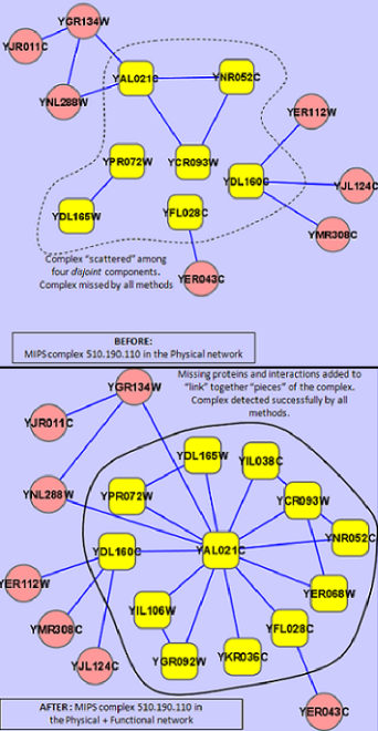
Figure 1: MIPS 510.190.110 complex before and after refinement using functional interactions by SPARC, and the effect on its detection using existing methods. BEFORE: The complex was “scattered” among four components; $CE$-score = 0.1905. AFTER: The four components were linked together into a single component; $CE$-score = 0.623.

While many additional complexes were detected using SPARC-based refinement, there were a few complexes that were missed as well (see Supplementary materials for a list). For example, the RNA polymerase complexes I, II and III, that are involved in the formation of RNA chains during transcription (Hurwitz, 2005), were bundled into a large dense module together with some of the TBP-associated factors and TFIID complexes, which are also involved in transcription (Green, 2000). Due to the functional similarity between the subunits of all these complexes, several functional interactions were added among them. Consequently, the methods recovered a large dense module housing all these complexes from which the individual complexes could not be segregated. The same was the case with the multi-eIF complexes and the SAGA-SLIK-ADA-TFIID complexes. The increase in the average cluster sizes in Table 8 further depict this effect.

Discussion

Functional interactions can be considered a “superset” of physical interactions. However, the low overlaps between the $P$ and $F$ networks seems to be projecting a suprisingly different picture ($|V(P)\cap V(F)|=2928$ and $|E(P)\cap E(F)|=1296$). The differential curation of the two datasets - the Physical dataset is inferred predominantly from experimental techniques while the Functional dataset is inferred predominantly from computational techniques - along with the presence of many missing (true negatives) and spurious (false positives) interactions, give rise to these low overlaps. Though this is an observation from only the two yeast datasets considered here, it may be worthwhile investigating how far away are we from the “ideal” picture of physical interactions being a proper subset of functional interactions in order to make most effective use of the two.

4 Conclusions

In this work, we attempt to reconstruct “sparse” complexes from PPI networks, a problem which has not been explored in previous works (see the recent survey by Li et al. (2010)) mainly because of the overused assumption that complexes form “dense” regions within the networks. Though this assumption might be valid, relying too much on it in the wake of insufficient PPI data makes it ineffective to detect sparse complexes. To counter this, we employ functional interactions, which again has not been tried before. This approach will particularly be effective in detecting complexes where a significant portion of the physical interactions are unknown or unreliable, for instance, in human. In addition to these, we also develop some theory around “complex derivability” (the CE score) that could be useful for developing new computational methods. For example, in the future we will looking at devising a new computational approach that selectively uses functional interactions by treating them differently from physical interactions.

References

- Ashburner et al. (2000) Ashburner, M., Ball C.A., Blake J.A., Botstein, D., Butler, H., Cherry, M., Davis, A.P., Dolinski, K., Dwight, S.S., Epigg, J., Harris, M.A., Hill, D.P., Issel-Tarver, L., Kasarkis, A., Lewis, S., Matase, J.C., Richardson, J., Ringwald, M., Rubin, G.M., Sherlock, G. (2010) ‘Gene ontology: a tool for the unification of biology’, Nature Genetics, Vol. 25, pp.25–29.
- Bader and Hogue (2003) Bader, G.D., Hogue, C.W.V. (2003) ‘Analyzing yeast protein-protein interaction data obtained from different sources’, Nature Biotechnology, Vol. 20, pp.991–997.
- Breitkreutz, et al. (2003) Breitkreutz, B., Stark, C., Tyers, M. (2003) ‘The GRID: The General Repository for Interaction Datasets’, Genome Biology, Vol. 4, pp.23.
- Cherry et al. (1998) Cherry, J.M., Adler, C., Chervitz S.A., Dwight S.S., Jia, Y., Juvik, G., Roe, T., Schroeder, M., Weng, S., Botstein, D. (1998) ‘SGD: Saccharomyces Genome Database’, Nucleic Acids Research, Vol. 26, pp.73–79.
- Chua et al. (2008) Chua, H., Ning, K., Sung, W., Leong, H., Wong, L. (2008) ‘Using indirect protein-protein interactions for protein complex prediction’, J. Bioinformatics and Computational Biology, Vol. 6, pp.435–466.
- Collins et al. (2007) Collins, S.R., Kemmeren P., Zhao, X.C., Greenbalt, J.F., Spencer F., Holstege, F., Weissman, J., Krogan, N.J. (2007) ‘Toward a comprehensive atlas of the physical interactome of Saccharomyces cerevisiae’, Mol. Cell. Proteomics, Vol. 6, pp.439–450.
- Cusick et al. (2008) Cusick, M.E., Yu, H., Smolyar, A., Venkatesan, K., Carvunis, A-R., Simonis, N., Rual, J-F., Borick, H., Braun, P., Dreze, M., Vandenhaute, J., Galli, M., Yazaki, J., Hill, D.E., Ecker, J.R., Roth, F.P., Vidal, M (2008) ‘Literature-curated protein interaction datasets’, Nature Methods, Vol. 6(1), pp.39–46.
- Green (2000) Green M.R. (2000) ‘TBP-associated factors (TAFIIs): multiple, selective transcriptional mediators in common complexes’, Trends Biochem Sci, Vol. 25, pp.59–63.
- Han et al. (2004) Han, J.D., Bertin, N., Hao, T., Goldberg, D., Berriz, G., Zhang, L.V., Dupuy, D., Walhout, A., Cusick, M.E., Roth, F., Vidal, M. (2004) ‘Evidence for dynamically organized modularity in the yeast protein-protein interaction network’, Nature, Vol 430, pp.88-93.
- Hurwitz (2005) Hurwitz, J. (2005) ‘The discovery of RNA polymerase’, J. Biological Chemistry, Vol. 280, pp.42477–42485.
- Jain and Bader (2010) Jain, S., Bader, G. (2010) ‘An improved method for scoring protein-protein interactions using semantic similarity within the gene ontology’, BMC Bioinformatics, Vol. 11, pp.562.
- Li et al. (2010) Li, X.L., Wu, M., Kwoh, C-K., Ng, S-K (2010) ‘Computational approaches for detecting protein complexes from protein interaction networks: a survey’, BMC Genomics, Vol. 11(S3).
- Liu et al. (2009) Liu, G., Wong, L., Chua, H.N. (2009) ‘Complex discovery from weighted PPI networks’, Bioinformatics, Vol. 25, pp.1891–1897.
- Mewes et al. (2006) Mewes, H.W., Amid, C., Arnold, R., Frishman, D., Guldener, U., Mannhaupt, G., Munsterkotter, M., Pagel, P., Strack, N., Stumpflen, V., Warfsmann, J., Ruepp, A. (2006) ‘MIPS: analysis and annotation of proteins from whole genomes’, Nucleic Acids Research, Vol. 34, pp.D169–D172.
- Newman and Girvan (2006) Newman, M.J., Girvan, M. (2004) ‘Finding and evaluating community structure in networks’, Physical Review, Vol. 69, pp.26113.
- Panasenko et al. (2006) Panasenko, O., Landrieux, E., Feuermann, M., Finka, A., Paquet, N., Collart, M. (2006) ‘The yeast CCR-NOT complex controls ubiquitination of the nascent-associated polypeptide (NAC-EGD) complex’, J. Biological Chemistry, Vol. 281, pp.31389–31398.
- Pereira-Leal et al. (2004) Pereira-Leal, J.B., Enright, A.J., Ouzounis, C.A. (2004) ‘Detection of functional modules from protein interaction networks’, Proteins, Vol. 54, pp.49–57.
- Pu et al. (2009) Pu, S., Wong, J., Turner, B., Cho, E., Wodak, S. (2009) ‘Up-to-date catalogues of yeast protein complexes’, Nucleic Acids Research, Vol. 37, pp.825–831.
- Shannon et al. (2003) Shannon, P., Markiel, A., Ozier O., Baliga, N.S., Wang, J., Ramage, D., Amin, N., Schwikowski, B., Ideker, T. (2003) ‘Cytoscape: a software environment for integrated models of biomolecular interaction networks’, Genome Research, Vol. 13, pp.2498–2504.
- Srihari et al. (2010) Srihari, S., Ning, K., Leong, H.W. (2010) ‘MCL-CAw: a refinement of MCL for detecting yeast complexes from weighted PPI networks by incorporating core-attachment structure’, BMC Bioinformatics, Vol. 11, pp.504.
- von Mering et al. (2003) von Mering, C., Huynen, M., Jaeggi, D., Schmidt, S., Bork, P., Snel, B. (2003) ‘STRING: a database of predicted functional associations between proteins’, Nucleic Acids Research, Vol. 12(1), pp.258–261.
- Wang et al. (2009) Wang, H., Kakaradov B., Collins S.R., Karotki, L., Fiedler, D., Shales M., Shokat, K.M., Walter, T., Krogan N.J., Koller, D. (2009) ‘A complex-based reconstruction of the Saccharomyces cerevisiae interactome’, Mol. Cell. Proteomics, Vol. 8, pp.1361–1377.
- Zhang et al. (2008) Zhang, B., Park, B.H., Karpinets, T., Samatova, N. (1998) ‘From pull-down data to protein interaction networks and complexes with biological relevance’, Systems Biology, Vol. 24, pp.979–986.