Gravitational lensing effects on sub-millimetre galaxy counts

Abstract

We study the effects on the number counts of sub-millimetre galaxies due to gravitational lensing. We explore the effects on the magnification cross section due to halo density profiles, ellipticity and cosmological parameter (the power-spectrum normalisation $\sigma_{8}$). We show that the ellipticity does not strongly affect the magnification cross section in gravitational lensing while the halo radial profiles do. Since the baryonic cooling effect is stronger in galaxies than clusters, galactic haloes are more concentrated. In light of this, a new scenario of two halo population model is explored where galaxies are modeled as a singular isothermal sphere profile and clusters as a Navarro, Frenk and White (NFW) profile. We find the transition mass between the two has modest effects on the lensing probability. The cosmological parameter $\sigma_{8}$ alters the abundance of haloes and therefore affects our results. Compared with other methods, our model is simpler and more realistic. The conclusions of previous works is confirm that gravitational lensing is a natural explanation for the number count excess at the bright end.

1 Introduction

Sub-millimetre galaxies (SMGs) at high redshift appear to be the counterparts of the most luminous star-forming galaxies in the local Universe. The high luminosity of these galaxies is presumed to be the result of large amounts of star formation, $100-1000\,h^{-1}\,M_{\odot}\,{\rm yr}^{-1}$ and warm dust (Blain et al. 2002). The millimetre and sub-millimetre wavelengths surveys have provided an important complement to the optical and radio searches for distant galaxies. In recent surveys, a significant population of high luminosity, high redshift galaxies have been discovered (Coppin et al. 2006; Negrello et al. 2007). The redshift distribution of the SMGs has a narrow distribution with a probable median redshift of $2-3$ (Chapman et al. 2005; Aretxaga et al. 2007). Surveys at sub-millimetre wavelengths show that the SMG population has a sharp falloff at the bright luminosity end of their luminosity function. Gravitational lensing by intervening galaxy clusters and groups modifies the observed number counts significantly (Blain 1996; Lima et al. 2010b; Jain & Lima 2011; Hezaveh & Holder 2011). Recently it has become possible to identify the lensed SMGs, e.g. from the ground with the South Pole Telescope (SPT) (Vieira et al. 2010), and from space with Herschel (González-Nuevo et al. 2012).

Gravitational lensing probes the cosmology, the mass distribution in the universe, and provides a way to study the high redshift objects (see Treu 2010 for a review). In the statistical study of cosmological gravitational lensing, several aspects have been studied: the lensing probability of separation of multiple images (e.g. Keeton & Madau 2001; Li et al. 2007); the number of giant arcs formed by gravitational lensing (e.g. Bartelmann et al. 1998; Li et al. 2005; Horesh et al. 2011) and the modified luminosity function (LF) of background sources (e.g. Lima et al. 2010b; Hezaveh & Holder 2011; Wyithe et al. 2011; Wardlow et al. 2012).

In this paper, we will focus on the LF of high redshift SMGs. There are a relatively large number of SMGs, and their redshift is likely high ($z>2$), both of which help to create an excellent source population for lensing studies (Chapman et al. 2005). To predict the observed source counts, the intrinsic LF needs to be known. Furthermore, in order to determine the probability (total cross section) of gravitational lensing, we need to know several properties of lens haloes, e.g. their abundance and internal structure, which are affected by the cosmological parameters of the universe. More specifically, the cross section due to gravitational lensing may be affected by halo ellipticity (e.g. Rusin & Tegmark 2001; Huterer et al. 2005), the radial profile of the lens halo (Li & Ostriker 2002; Oguri & Keeton 2004) as well as the size of background galaxies (Perrotta et al. 2002; Hezaveh & Holder 2011). In Lima et al. (2010a), haloes are modelled with NFW profiles, while ellipticity is added to their lensing potential to increase the lensing probability. More recently, Lapi et al. (2012), considered a composite model for galactic sized halo, where dark matter is modelled as NFW and the stellar component by a Sersic profile (Sérsic 1963). It is in fact close to the isothermal profile. They also use the public code GLAFIC from Oguri (2010) to study the effect of halo ellipticity on the lensing cross section and find that the ellipticity only weakly affects the cross section of the isothermal halo lens. Our analytical results confirm their finding.

Axisymmetric lensing models offer simplicity in the study of lens statistics. Several spherical lenses have been studied, such as the Singular Isothermal Sphere (SIS) and the Navarro-Frenk-White profile (e.g. Li & Ostriker 2002; Oguri & Keeton 2004). Due to baryonic cooling, clusters and galaxies will have different mass profiles. Therefore, a combination of two population halo mass profiles will be studied in this work. The statistical effect of lensing will be affected by the cooling mass scale $M_{\rm cool}$ (see, e.g., the study on multiple images and image splitting by Li & Ostriker 2002; Chen 2004). A cooling mass scale of $\sim 10^{13}\,h^{-1}\,M_{\odot}$ has been suggested (see, e.g., Porciani & Madau 2000; Kochanek & White 2001). On large scales the mass function of dark haloes relates to the primordial fluctuations of the universe, which can be characterised by the power-spectrum normalisation parameter $\sigma_{8}$. Thus, the total cross section will be sensitive to this parameter as well. Moreover, previous studies have shown that different aspects also affect the lensing efficiency, like the substructures within the dark haloes (Oguri 2006), central massive black holes (Mao & Witt 2012; Li et al. 2012) and external shear (Huterer et al. 2005). Most of them probably do not play significant roles, and so they will not be considered in this paper.

We will study the lensing efficiency, i.e. the magnification cross section in this paper. We start from a single lens halo for different halo profiles, and present the lensing cross section dependence on halo properties. We show that the halo ellipticity does not affect the cross section significantly, while the halo density profile does. As we mentioned before, a combination of halo profiles is more physical and we find such a scenario can produce a higher lensing probability than a single universal NFW profile. We present our calculation and employ it to study the luminosity function in Section 3; we further discuss our results in Section 4. The cosmology that we adopt in this paper is a $\Lambda$CDM model with parameters based on the results of the Wilkinson Microwave Anisotropy Probe seven year data (Komatsu et al. 2011): $\Omega_{\Lambda}=0.734$, $\Omega_{\rm m}=0.266$, $\Omega_{\rm b}=0.0449$, $n=0.963$, a Hubble constant $H_{0}=100h$ km s^-1 Mpc^-1 and $h=0.71$. We allow the $\sigma_{8}$ parameter to vary, but use the WMAP7 value $\sigma_{8}=0.8$ if not mentioned.

2 Basic Formalism

The fundamentals of gravitational lensing can be found in Bartelmann & Schneider (2001). For its elegance and brevity, we shall use the complex notation. The thin-lens approximation is adopted, implying that the lensing mass distribution can be projected onto the lens plane perpendicular to the line-of-sight. We introduce angular coordinates $\theta$ with respect to the line-of-sight. The lensing convergence, that is the dimensionless projected surface-mass density, can be written as

$$\kappa(\mbox{\boldmath$\theta$})=\Sigma(\mbox{\boldmath$\theta$})/\Sigma_{\rm cr},\;\;\;{\rm where}\;\;\;\Sigma_{\rm cr}=\frac{c^{2}}{4\pi G}\frac{D_{\rm s}}{D_{\rm d}D_{\rm ds}}\;$$ (1)

is the critical surface mass density depending on the angular-diameter distances $D_{\rm s}$, $D_{\rm d}$ and $D_{\rm ds}$ from the observer to the source, the observer to the lens, and the lens to the source, respectively. $\Sigma(\mbox{\boldmath$\theta$})$ is the projected surface-mass density of the lens. All lensing quantities can be derived from the effective lensing potential $\psi$,

$$\psi(\mbox{\boldmath$\theta$})=\frac{1}{\pi}\int_{{\cal R}^{2}}\mathrm{d}^{2}\theta^{\prime}\kappa(\mbox{\boldmath$\theta$}^{\prime})\;{\rm ln}|\mbox{\boldmath$\theta$}-\mbox{\boldmath$\theta$}^{\prime}|\;.$$ (2)

To the lowest order, image distortions caused by gravitational lensing are described by the complex shear

$$\gamma=\frac{1}{2}\left(\partial_{1}^{2}\psi-\partial_{2}^{2}\psi\right)+{\rm i}\partial_{1}\partial_{2}\psi\;.$$ (3)

The magnification for a point source is given by

$$\mu=\dfrac{1}{(1-\kappa)^{2}\,-\,|\gamma|^{2}}.$$ (4)

2.1 Lensing properties of different dark matter halo profiles

Having laid out a general formalism, we will present the basic lensing properties of two different dark matter halo profiles that will be used in this paper (see below). They are Singular Isothermal Sphere (SIS) and Navarro-Frenk-White (NFW, Navarro et al. 1997) profiles.

The dimensionless surface mass density and shear for an SIS halo are

$$\kappa=\frac{\theta_{\rm E}}{2\theta}\;,\;\;\;\;\;\gamma=-{\theta_{\rm E}\over 2\theta}{\rm e}^{2\mathrm{i}\phi},$$ (5)

where $\phi$ is the position angle around the lens, $\theta=\sqrt{\theta_{1}^{2}+\theta_{2}^{2}}$ is the angular separation, and $\theta_{\rm E}$ is the Einstein angular radius, which is calculated by

$$\theta_{\rm E}=4\pi\left(\sigma_{v}\over c\right)^{2}{D_{\rm ds}\over D_{\rm s}},$$ (6)

where $\sigma_{v}$ is the one-dimensional velocity dispersion, and $c$ is the speed of light. In the rest of the paper, $c$ is used as the concentration parameter. The lensing properties of the NFW profile has been calculated by Bartelmann (1996). The convergence is analytically given by

$$\kappa=2\kappa_{s}{f(x)\over x^{2}-1},$$ (7)

where $x=\theta D_{\rm d}/r_{s}$ (or $x=\theta/\theta_{s},\theta_{s}=r_{s}/D_{\rm d}$) is the dimensionless radius, and the function $f(x)$ is defined as

$$f(x)=\begin{cases}1-\dfrac{{\rm arcsech}x}{\sqrt{1-x^{2}}}\;\;(x<1);\\ \\ 0\quad\quad\quad\quad\quad\;\;\;(x=1);\\ \\ 1-\dfrac{{\rm arcsec}x}{\sqrt{x^{2}-1}}\;\;(x>1).\\ \end{cases}$$ (8)

The physical properties of the halo are contained in the parameter $\kappa_{s}=\rho_{\rm crit}\Delta_{c}r_{s}/\Sigma_{\rm cr}$, where $\Delta_{c}$ is the dimensionless characteristic density and $\rho_{\rm crit}$ is the critical density. The halo mass is defined as $M_{200}=800/3\rho_{\rm crit}\pi r_{200}^{3}$, where $r_{200}=r_{s}\,c$ and $c$ is the concentration parameter (see the appendix in Navarro et al. 1997). More lensing properties of the NFW halo profile can be found in Wright & Brainerd (2000).

2.2 Lensing cross sections of dark matter haloes

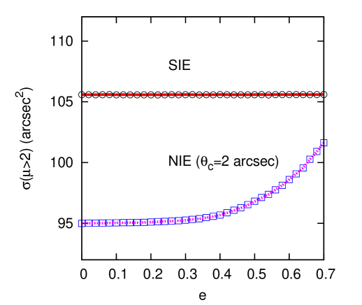
Figure 1: Cross section $\sigma(\mu>2)$ vs. halo ellipticity for the SIE and NIE halo profiles. The solid line is the analytical result for the SIE halo given by Eq. 10. The open circles and dashed line are the cross section using cell counts in the magnification map, where the magnification is derived by Eqs. 9 and 28 for SIE and NIE model respectively. The open squares represent the numerical results for the NIE halo which magnification is derived numerically (Appendix B). $\theta_{\rm E}=5.5$ arcsec is used here for all cases (which corresponds to the halo mass of $M_{200}=10^{14}\,h^{-1}\,M_{\odot}$). For the NIE halo, a core radius $\theta_{c}=2$ arcsec is used.

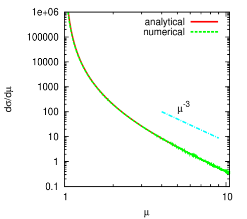
Figure 2: Differential lensing cross section as a function of magnification $\mu$ for the SIE halo. $\theta_{\rm E}=5.5$ arcsec is used as in Fig. 1. The solid and dashed lines are the analytical and numerical results, which almost overlap. The dot-dashed line shows the expected asymptotic behaviour.

We will calculate the cross section of different halo profiles, and present their dependence on different parameters, e.g. halo ellipticity and concentration etc. Some previous studies have shown that the magnification cross section increases with halo ellipticity dramatically (e.g. Lima et al. 2010a). We, however, find that this is mainly because the halo mass is also changed. We start with an elliptical surface density for which the mass within an ellipse is identical with that of the axis-symmetric one. In general, the corresponding magnification can be calculated numerically (Schramm 1990).

We first perform a series of tests for the cross section of the halo ellipticity. The halo ellipticity is characterised by $e=1-q$, where $q=\theta_{a}/\theta_{b}$ is the axis ratio, $\theta_{a}$ and $\theta_{b}$ are the major and minor axes, respectively. The angular separation $\theta$ will be replaced by $\Theta=\sqrt{q\theta_{1}^{2}+\theta_{2}^{2}/q}$ (uppercase $\Theta$ is used for the elliptical coordinate) in Eq. 5 to calculate $\kappa$ and $\gamma$ for a Singular Isothermal Ellipsoid (SIE) halo (see Keeton & Kochanek 1998 for more details on the lensing properties of an SIE halo). It is a radial coordinate and will be constant on elliptical contours (thus $x=\Theta D_{\rm d}/r_{s}$ in the NFW model). The total mass within a given $\Theta$ is invariant with the ellipticity $e$. Following Eq. 28, the magnification of an SIE halo has an analytical expression

$$\mu={\Theta\over\Theta-\theta_{\rm E}}.$$ (9)

For a given magnification $\mu_{\rm min}$, the cross section $\sigma(\mu)$ is the area inside which the magnification of a source is equal to or larger than $\mu_{\rm min}$ on the source plane. For the SIE halo, the cross section can be given analytically

$$\sigma(\mu)=\pi\theta_{\rm E}^{2}\left({1\over(\mu-1)^{2}}+{1\over(\mu+1)^{2}}\right).$$ (10)

Notice that at large magnification, the cross section follows the predicted asymptotic power-law $1/\mu^{2}$ for $\mu\gg 1$ (Schneider et al. 1992).

The mass of the SIE halo is related to $\theta_{\rm E}$. For the SIE model the mass is related to the rotation velocity, which can be calculated using $M_{200}=V_{c}^{3}/(10GH(z))$ (Mo et al. 1998). The relation between the rotation velocity and velocity dispersion is complicated and may be different for different types of galaxies. We use the approximate relation between the rotation velocity and the velocity dispersion $\sigma_{v}=V_{c}/\sqrt{2}$, which is suggested by Chae (2010). The cross section has an expression of mass and distance

$$\sigma(\mu) = {16\pi^{3}\over c^{4}}\left(25\over 2\right)^{2/3}\left(GHM_{200}\right)^{4/3}\left(D_{\rm ds}\over D_{\rm s}\right)^{2}$$ (11)

$$\left({1\over(\mu-1)^{2}}+{1\over(\mu+1)^{2}}\right).$$

In our definition of the ellipticity, the mass and the cross section do not change with ellipticity. We can see that only the halo mass and the redshifts of lens and source affect the cross section. In the appendix, one can find more analytical results for the magnification and cross section of SIE and Non-singular Isothermal Ellipsoid (NIE) profiles.

To check the accuracy of Eq. 10, we create a magnification map using Eq. 9 and sum up the pixels following Eq. 29. A halo with mass of $M_{200}=10^{14}\,h^{-1}\,M_{\odot}$ is used, which gives $\theta_{\rm E}=5.5$ arcsec for $z_{\rm d}=0.5$ and $z_{\rm s}=2.0$. The resolution of the magnification grid is $\Theta_{\rm E}/500$. We increase the lens halo ellipticity to see its effect to the cross section. For simplicity, we use a constant halo ellipticity as a function of radius. The numerical results are shown by the open circles in Fig. 1 and the red solid line shows the prediction of Eq. 10. We can see that the results agree well with each other. It encourages us to explore whether such an independence is also valid for other kinds of mass distribution models. Fig. 2 presents the probability of cross section as a function of magnification for the SIE halo ($\mathrm{d}\sigma/\mathrm{d}\mu$). The solid line represents the theoretical prediction, while the dashed line is obtained by numerical calculation. One can see that the numerical result closely follows the theoretical prediction. As expected, at small $\mu$ the probability density distribution rapidly decreases; at large $\mu$, it becomes close to the asymptotic relation $\propto\mu^{-3}$.

By adding a core of $\theta_{c}=2$ arcsec into the SIE model, we extend our test to the NIE model. In Appendix A, we show an analytical expression of the magnification (Eq. 28). By summing up the pixels in the magnification map as before, we show the “theoretical” cross section as a dashed line in Fig. 1. We call it the theoretical cross section because the magnification is calculated analytically. We also show the result where the magnification is calculated numerically. One can see that the cross section of NIE halo increases with the ellipticity by a few percent for the parameters considered here.

For most elliptical mass distribution models, the magnification can not be derived analytically, e.g., the Einasto model (Retana-Montenegro et al. 2012), the Hernquist model (Baes & Dejonghe 2002) and the NFW model. Schramm (1990) proposed a way to calculate the lensing properties for any kind of elliptical mass model. This algorithm is summarised in Keeton (2001) and revised for our definition of elliptical coordinate in Appendix B. Following this approach, we recalculate the magnification numerically for the NIE halo and plot the results in Fig. 1 as the open squares. The good agreement between the dashed line and the open squares guarantees the accuracy of the numerically calculated magnification and confirms the weak dependence between the cross section and the ellipticity.

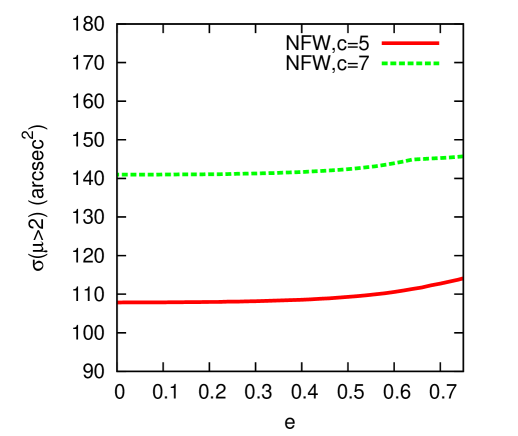
Figure 3: Cumulative cross section $\sigma(\mu>2)$ vs. halo ellipticity for the NFW halo profiles: The solid (dashed) line is the result for the NFW halo profile with concentration $c=5$ ($c=7$). The same condition, halo mass $M_{200}=10^{14}\,h^{-1}\,M_{\odot}$ and redshift $z_{d}=0.5$, $z_{s}=2.0$ are used for all the figures in this section.

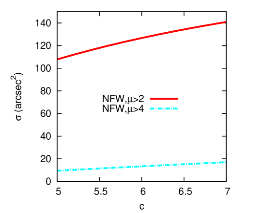
Figure 4: Lensing cross section vs. concentration for the NFW profiles. The solid line is the normalised cross section of $\mu>2$ for NFW profiles. The dotted line is for the cross section with $\mu>4$. The same halo mass $M_{200}=10^{14}\,h^{-1}\,M_{\odot}$ is used.

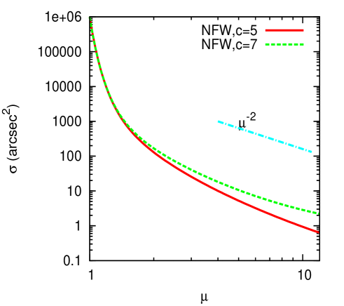
Figure 5: Lensing cross section vs. $\mu$ for the NFW profile. The solid and dashed lines represent the results for the NFW profile with $c=5,7$. Again a halo mass $M_{200}=10^{14}\,h^{-1}\,M_{\odot}$ is used.

For an elliptical NFW (eNFW) halo, the lensing properties, e.g. shear, magnification and the cross section, can be calculated numerically as above. We perform similar numerical tests for the cross section $\sigma(\mu)$ using eNFW halo profiles. The same mass $M_{200}=10^{14}\,h^{-1}\,M_{\odot}$ and redshifts ($z_{d}=0.5$, $z_{s}=2.0$) are used.

In Fig. 3, we show the cross section $\sigma(\mu>2)$ variation with halo ellipticity. Two different concentration parameters $c=5,7$ are used for NFW halo profiles. We find that there is a weak dependence on the halo ellipticity of $\sigma$ (less than $5$ percent). Fig. 4 shows the cross section variation with the concentration parameter $c$ for the NFW profiles. As expected, with a higher concentration the lensing efficiency is higher. Fig. 5 shows the cross section $\sigma(\mu)$ dependence on the magnification $\mu$. At high magnification, there is a significant difference in cross section between two concentration parameters for the NFW profile.

There are a number of complications we have ignored (see also the discussion). The numerical tests we performed only take into account the projected shape, and assumed the ellipticity is constant as a function of radius. In reality, this may not be true. In particular, irregular shape lens haloes may have different cross sections and probability of generating multiple images especially for the massive haloes not long after the merging event. Other properties, such as the substructures may also affect the cross section. The finite source size may smooth the magnification and lowers the lensing efficiency (see the end of Section 3). Thus, in reality, the lensing halo may have slightly different cross sections, which need to be further studied using numerical simulation, although the required spatial and mass resolutions may be challenging. As the effect of ellipticity on the lensing cross section seems to be relatively small, in this paper, for simplicity we will adopt the spherical lens model in the following calculations.

2.3 Probability function of magnification

The probability distribution $P(\mu)$ can be estimated either by ray-tracing simulations (e.g. Hilbert et al. 2007), or by semi-analytical methods (e.g. Lima et al. 2010b), which integrates all the halo contributions along the line of sight from us to the source redshift. We will adopt the latter approach, which allows us to easily test the dependence on parameters, e.g. $\sigma_{8}$ and $M_{\rm cool}$.

Different halo density profiles will be employed for lens haloes, i.e. SIS and NFW. The mass-concentration relation for the NFW halo profile has been studied by several authors (e.g. Bullock et al. 2001; Zhao et al. 2009). In this paper, we adopt the simple model

$$c(M,z)={9\over 1+z}\left(M\over M_{*}\right)^{-0.13},$$ (12)

where $M_{*}$ is calculated by $\sigma_{m}(M_{*})=\delta_{c}$. $\sigma_{m}^{2}(M)$ is the variance of the linear density field (Eq. 15), and $\delta_{c}$ is the linearly extrapolated density contrast threshold at redshift $z$ in spherical collapse, here we use $\delta_{c}(z=0)=1.686$.

The halo mass function (Press & Schechter 1974), which determines the number of haloes given a mass at each redshift $n(M,z)$, can be written as

$${\mathrm{d}n\over\mathrm{d}M}\mathrm{d}M={\bar{\rho}\over M}f(\nu)\mathrm{d}\nu,$$ (13)

where $\bar{\rho}$ is the comoving mean matter density of the Universe and $\nu=\delta_{c}/\sigma_{m}(M)$. In the Sheth & Tormen (1999) formalism, we have,

$$\nu f(\nu)=A\sqrt{\dfrac{2}{\pi}a\nu^{2}}\left[1+(a\nu^{2})^{-p}\right]{\rm exp}\left[-a\nu^{2}/2\right].$$ (14)

Here $\sigma_{m}^{2}(M)$ is the variance of the linear density field in a top hat of radius $r$ that encloses $M=4\pi r^{3}\rho_{m}/3$ at the background density

$$\sigma_{m}^{2}(r)=\int\dfrac{\mathrm{d}^{3}k}{(2\pi)^{3}}|W(kr)|^{2}P_{L}(k),$$ (15)

where $P_{L}(k)$ is the linear power spectrum

$$P_{L}(k,z)\propto k^{n}D^{2}(z)T^{2}(k),$$ (16)

and $W(kr)$ is the Fourier transform of the top hat window function. The fitting formula of the linear transfer function including baryons (Eisenstein & Hu 1998) is used here and we use the WMAP 7-year cosmology (Komatsu et al. 2011). Alternative models for the shape of $n(M,z)$ are available in the literature (e.g. Matarrese et al. 2000), we will not consider these since Eq. (14) provides a good description of the mass function in numerical simulations. We however use another form of Eq. (14) which is easier to implement in numerical integration

$$f(\sigma,z)\equiv{M\over\bar{\rho}}{\mathrm{d}n\over\mathrm{d}{\rm ln}\sigma^{-1}}.$$ (17)

It has a fitting formula of

$$f(\sigma)=0.315\,{\exp}(-|{\ln}\,\sigma^{-1}+0.61|^{0.38})$$ (18)

in the range $-1.2\leq{\ln}\,\sigma^{-1}\leq 1.05$ (Jenkins et al. 2001).

The lensing cross section $\sigma(>\mu,z_{d},M)$ for a single halo will be calculated as a function of mass. The halo mass is used as $M_{200}$. The cross section of the SIS halo can be calculated analytically (Eq. 10) and that of the NFW halo will be performed numerically. The sum of all cross sections in the Universe can be written as (Lima et al. 2010a)

$$\sigma_{\rm tot}(\mu)=4\pi\int{D_{A}^{2}(z_{d})\over H(z_{d})}\,\mathrm{d}z_{d}\int\mathrm{d}M{\mathrm{d}n(z_{d},M)\over\mathrm{d}M}\;\sigma(>\mu,z_{d},M),$$ (19)

where $D_{A}$ is the comoving angular diameter distance, and we make a simplification that the source SMGs are distributed at a fixed redshift. We place the sub-millimetre source galaxies mostly at redshift $z_{s}=3.0$ (Chapman et al. 2005; Yan et al. 2007), but will later allow it to vary between $2-4$ (see Section 3). The lens haloes are distributed between the sources and us ($0.001<z_{d}<1.5$).

The total cross section is integrated using Eq. 19, then the cumulative probability that a source at $z_{s}$ is magnified by a factor greater than $\mu_{\rm min}$ is then

$$P(\mu)={\sigma_{\rm tot}(\mu)\over 4\pi}.$$ (20)

The probability density can be obtained by $p(\mu)=-\mathrm{d}P(\mu)/\mathrm{d}\mu$. The magnification probability function will be affected by several aspects, e.g. the lens halo profile, halo mass function, and the lens and the source redshifts etc. We will study several factors. First of all, the cross section of a single halo $\sigma(>\mu,z_{d},M)$ can be calculated using different models. We perform the calculation for three profiles: 1) the SIS halo profile, 2) the NFW halo profile, and 3) a two population combination of SIS and NFW profiles where the transition occurs at the cooling mass scale $M_{\rm cool}$ between galaxies and clusters.

In the left panel of Fig. 6, one can see that the lens halo profile will affect the probability function $p(\mu)$. All the results follow $p(\mu)\propto\mu^{-3}$ as expected when $\mu\gg 1$. At small $\mu$, all the profiles generate similar lensing probability and all the curves drop rapidly with increasing $\mu$. The SIS model will generate a larger probability for large $\mu$; when $\mu$ approaches to $1$, the SIS model has a slightly smaller probability than the NFW profile. The result using SIS+NFW however is close to that of the NFW profile. The reason is that the main difference between SIS and NFW is for large $\mu$, and the main contribution to large $\mu$ is from massive haloes, i.e. the NFW haloes here.

As expected, the transition mass $M_{\rm cool}$ also affects the probability function. For a larger $M_{\rm cool}$, there will be more lenses modeled as SIS, as a result one will obtain a higher probability at large $\mu$ (middle panel in Fig. 6). In particular, we find that the probability is about $10\%$ lower if we use $M_{\rm cool}=10^{12}\,h^{-1}\,M_{\odot}$ at large $\mu$ than the case with $M_{\rm cool}=10^{13}\,h^{-1}\,M_{\odot}$; at small $\mu$ there is a few percent difference. In the right panel of Fig. 6, one can see that a larger $\sigma_{8}$ increases the lensing probability due to a larger number of massive structures. The difference exists for most $\mu$, although it is more significant for large $\mu$ ( $\sim 25\%$) than for smaller $\mu$ ($\sim 10\%$).

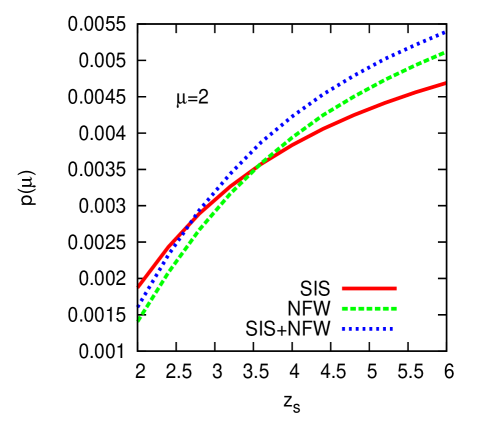
Figure 7: Lensing probability density $p(\mu=2)$ from intervening haloes ($0.001<z_{d}<1.5$) for different source redshift $z_{s}$. The solid, dashed and dotted lines represent the probabilities for the SIS, NFW and SIS+NFW profiles respectively.

In addition, we use different source redshifts. The same lens halo redshifts are used ($0.001<z_{\rm d}<1.5$), since at high redshift, the number density of lens halo will dramatically decrease. In Fig. 7, we can see that the lensing probability increases with the source redshift; at large redshift it increases more slowly. At very high redshifts (e.g., $z_{s}>5.0$), the luminous source number density is low, thus high redshift sources will not strongly affect our result. Moreover, different halo profiles have different source redshift dependence. The probability of NFW profiles increase faster than that of SIS profile.

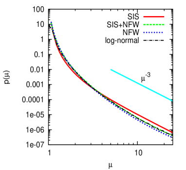
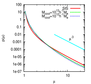
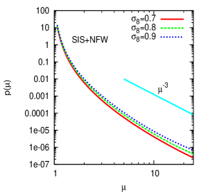
Figure 6: Lensing probability density $p(\mu)$ along the line of sight up to $z_{s}=3.0$ from all intervening haloes. Left: Results using different halo profiles of SIS, SIS+NFW and NFW are shown as the red solid, green dashed, and blue short dashed lines respectively. $M_{\rm cool}=10^{13}\,h^{-1}\,M_{\odot}$ is used. The black dot-dashed line represents the combined probability of log-normal approximation (Hilbert et al. 2011) and SIS+NFW. Middle: Results for the SIS+NFW halo profile using different $M_{\rm cool}$’s: $10^{13}\,h^{-1}\,M_{\odot}$ (green dashed line), $10^{12}\,h^{-1}\,M_{\odot}$ (blue short dashed line). Right: Results for SIS+NFW halo profile using different $\sigma_{8}$’s: $\sigma_{8}=0.7$ (red solid line), $\sigma_{8}=0.8$ (green dashed line), $\sigma_{8}=0.9$ (blue short dashed line). In all three panels, the green dashed line represents the result using the same parameters (SIS+NFW halo, $M_{\rm cool}=10^{13}\,h^{-1}\,M_{\odot}$ and $\sigma_{8}=0.8$) for better comparisons.

3 Number counts of sub-millimetre galaxies

The intrinsic number density distribution of a population of galaxies can be fitted by empirical or semi-analytical models (Baugh et al. 2005). In this paper we adopt a Schechter (1976) form for the intrinsic luminosity function:

$${\mathrm{d}n\over\mathrm{d}S}={n^{*}\over S^{*}}\left(S\over S^{*}\right)^{\alpha}{\rm e}^{-S/S^{*}},$$ (21)

where $n^{*}$, $S^{*}$, and $\alpha$ are free parameters. Lensing by intervening haloes changes the intrinsic $\mathrm{d}n/\mathrm{d}S$ to its observed counterpart. In addition to making sources appear brighter, gravitational lensing also dilutes the source number density by magnifying the observed solid angle. As discussed in Jain & Lima (2011), the observed number counts for the whole population is

$${\mathrm{d}n\over\mathrm{d}S}={1\over\langle\mu\rangle}\int{1\over\mu^{\prime}}{\mathrm{d}p\over\mathrm{d}\mu^{\prime}}{\mathrm{d}n^{\prime}\over\mathrm{d}S^{\prime}}\left(S^{\prime}=S/\mu^{\prime}\right)\mathrm{d}\mu^{\prime}.$$ (22)

The probability at small magnification is difficult to calculate using the halo model. We perform the integral (Eq.22) from $\mu_{\rm min}=1.1$ to $\mu_{\rm max}=30$, and use probability $(1-P_{0})\delta(\mu=1)$ for $\mu<\mu_{\rm min}$, where $P_{0}$ is the cumulative probability in image plane from $\mu_{\rm min}$ to $\mu_{\rm max}$, and $\delta(\mu=1)$ is the Dirac function. We discuss how the choice of $\mu_{\rm min}$ affects the results at the end of this section.

First, we compare our prediction with the results given in the right panel of Fig. 2 in Lima et al. (2010b). We used the rescaled intrinsic Schechter function

$${\mathrm{d}N^{\prime}\over\mathrm{d}S^{\prime}}=S^{\prime\alpha}{\rm e}^{-S^{\prime}},$$ (23)

where $N^{\prime}=n/n^{*}$ and $S^{\prime}=S/S^{*}$. Different $n^{*}$ and $S^{*}$ are used for different wavelengths (for more detail see Lima et al. 2010b). We adopt a combination of spherical NFW and SIS halo profiles for lens and show our prediction in Fig. 8. The rescaled luminosity functions before and after lensing are shown by the lines and the points are the rescaled data using different wavelengths and different surveys. One can see that our result can match the data as well as the model prediction of Lima et al. (2010b). From the view of methodology, our model is simpler and more meaningful. Their model has to adopt a high ellipticity of halo (e.g. $0.4$) to reach the required lensing efficiency. We also show the effect of the transition mass $M_{\rm cool}$. We allow $M_{\rm cool}$ to vary from $10^{12}\,h^{-1}\,M_{\odot}$ to $10^{14}\,h^{-1}\,M_{\odot}$. The predicted uncertainty is shown by the shaded region. The model with a larger $M_{\rm cool}$ will predict a higher number count at the bright end due to more effective SIS halo lenses.

We then apply our method to calculate the sub-millimetre galaxy counts of HerMES observation. We use $n^{*}=5\times 10^{3}/$deg², $S^{*}=10$ mJy and $\alpha=-1.0$ obtained by fitting the low flux data points (Glenn et al. 2010). In Figs. 9 and 10 the lines show the luminosity function before and after lensing. Here we mainly consider a source redshift $z_{s}=3.0$. The SIS profile will generate more lensed images than the NFW profile. The points show the HerMES data (HerMES Collaboration et al. 2012) to compare with our predictions. Similar as Fig. 6, different models are compared. Lensing does not significantly affect the galaxy number counts at low luminosity, while at the bright end, lensing dramatically enhances the number counts. But all the predictions with our model (sources at redshift $z_{s}=3.0$, $\sigma_{8}=0.8$ and $M_{\rm cool}=10^{13}\,h^{-1}\,M_{\odot}$) have lower number counts than that observed by HerMES. Wardlow et al. (2012) also investigated the lensing effect on the HerMES SMG data and find that this discrepancy is mainly due to the contamination from the late-type sprials. Although our lensing efficiency has been enhanced by the SIS halo, the discrepancy is still significant. The number of lensed SMGs in which these sprial galaxies have been subtracted (Wardlow et al. 2012) is shown as the solid points in the figure. Our results confirms that gravitational lensing is a natural way to explain the behaviour of SMG luminosity function at the bright end.

In Fig. 9, the shaded region shows the uncertainty due to source redshift between $2.0$ and $4.0$. All of our predictions with a single source redshift are larger than the lensed data (solid points). In reality, the source will have a redshift distribution. Different source redshift distributions are suggested due to different selection criteria. A significant number of low redshift sources are also found in the Herschel survey (e.g. Casey et al. 2012). Furthermore, the Schechter luminosity function parameters such as $S^{*}$ or $\alpha$ may be different as well. So a more realistic prediction will depend on these unknown parameters, nevertheless the agreement is encouraging.

In Fig. 10, we show the effects due to cosmological parameter $\sigma_{8}$. As one expects, a large $\sigma_{8}$ will increase the halo number density for all masses, which will increase the lensed galaxy number counts at both bright and faint ends. From the shaded regions in Figs. 8, 9 and 10, one can see that the uncertainty of source redshift affects our result the most.

In addition, we perform our calculation using different $\mu_{\rm min}$ ($1.05$ and $1.15$). The effects on the number counts are small, $5\%$ at the bright end and $7\%$ at the faint end. In Hilbert et al. (2011), a log-normal approximation of lensing probability is found using large volume numerical simulations. We use the fitting formula given by Hilbert et al. (2011) to calculate the probability for $\mu<1.1$. We perform the integral from $\mu_{\rm min}=0.01$ to $\mu_{\rm max}=30$ and find that the change to the number counts at the bright end is also small (blue line in Fig. 10). The upper limits $\mu_{\rm max}$ is uncertain as well. Perrotta et al. (2002) consider the SMG population and estimate $\mu_{\rm max}\sim 10-30$. However, a magnification of $\mu\sim 45$ is reported in the cluster Abell 2218 (Kneib et al. 2004). Our results show that it causes a decrease of $50\%$ at the bright end ($S>0.1$ Jy) if we adopt $\mu_{\rm max}=20$ but keep the faint end unchanged. This effects will be blurred if the finite source size of background galaxies is taken into account and therefore needs a more detailed study.

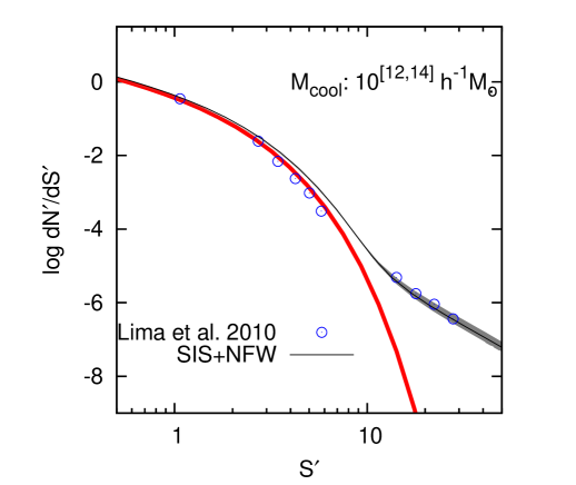
Figure 8: The scaled intrinsic and lensed galaxy number counts $\mathrm{d}N^{\prime}/\mathrm{d}S^{\prime}$: the solid red line is the intrinsic Schechter luminosity function. The black line with grey shaded region represents the lensed galaxy number count due to the combination of halo profiles for sources at redshift $z_{s}=3.0$, and the shaded region displays the range of lensing predictions due to different transition masses $M_{\rm cool}$. The open circles are data points from the right panel of Fig. 2 in Lima et al. (2010b).

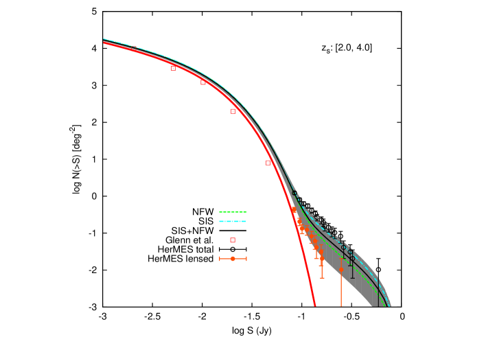
Figure 9: Intrinsic and lensed galaxy number counts: the red thick solid line is the intrinsic Schechter luminosity function describing galaxy number counts. The other lines represent the lensed galaxy number counts due to different lens halo profiles: SIS (cerulean dot-dashed line), NFW (green dashed line) and SIS+NFW (dark solid line), assuming that all the source galaxies are at redshift $z_{s}=3.0$. The shaded region displays the range of prediction due to different source redshifts (from $z_{s}=2.0$ to $z_{s}=4.0$). The points are cumulative $500$ $\mu$m number counts for HerMES blank-field catalogs (Oliver et al. 2010; HerMES Collaboration et al. 2012) and $P(D)$ analysis (Glenn et al. 2010).

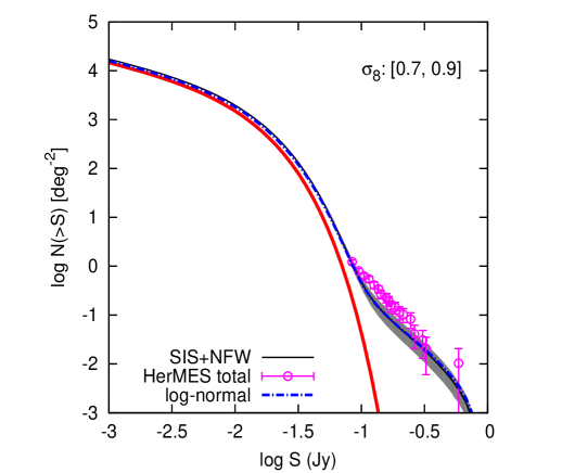
Figure 10: Similar to Fig. 9, comparison of different $\sigma_{8}$’s: the solid dark line is the result of SIS+NFW halo with $\sigma_{8}=0.8$ assuming $z_{s}=3.0$ and $M_{\rm cool}=10^{13}\,h^{-1}\,M_{\odot}$. The shaded region displays the range of predictions due to different $\sigma_{8}$ values (from $\sigma_{8}=0.7$ to $\sigma_{8}=0.9$). The blue line represents the result of combination of log-normal approximation and SIS+NFW (see end of section 3 for more detail).

4 Summary and Discussion

In this paper we have studied the lensing effects of galaxy and cluster haloes, and how lensing will change the luminosity function of high redshift sub-millimetre galaxies. The lensing properties for individual haloes and haloes as a population have been presented. In particular, we find that the halo ellipticity does not affect the lensing efficiency significantly with our definition of ellipse coordinate. On the other hand, as expected, halo mass profiles significantly affect the lensing cross section. Not surprisingly, the NFW profile has lower lensing efficiency than the SIS profile. We argued that a combination of two population of halo profiles is more realistic: we use the SIS model for mass less than $M_{\rm cool}$ and NFW for mass greater than $M_{\rm cool}$. The SIS profile is favoured for galactic sized haloes, due to the baryonic cooling effect. It is also close to the composite profile of an NFW dark halo and a Sersic stellar component Gavazzi et al. (2007); Lapi et al. (2012). Our prediction with simple assumptions (two population, circular symmetric halo profile) can match the observation given in Lima et al. (2010b) quite well. Compared with previous works, our model is simpler and more realistic. For the SMG number counts of (HerMES Collaboration et al. 2012), the excess on the bight end can not be explained by lensing alone. The contamination from local late-type sprial galaxies is non-negligible. On the other hand, the cleaned lensed SMGs sample can be easily fit by lensing. We vary $M_{\rm cool}$ between $10^{12}$ and $10^{13}\,h^{-1}\,M_{\odot}$, and find it only slightly affects the lensing probability. Moreover, our results also show the dependence of the lensing probability on the cosmological parameter, $\sigma_{8}$. This is especially important for large magnifications, since in the halo model, the number density of massive haloes is sensitive to $\sigma_{8}$.

In a simple test of total cross section as a function of halo mass, we find that most contribution to the lensing cross section comes from dark matter haloes with mass between $10^{12}$ and $10^{15}\,h^{-1}\,M_{\odot}$, i.e. massive galaxies or galaxy groups. The upper mass limit is due to the rare number of massive haloes. It also explains why most lenses are at low redshift, since massive haloes have not yet formed at earlier times. The lower limit is due to the small cross sections of individual low-mass lens haloes, because they generate little cross sections.

Our model is simplistic, a number of improvements can be made. (1) We did not take into account the additional matter distribution between the source and observer, i.e. several small haloes may contribute to a modest lensing magnification. The contribution to the cross section appears to be small, e.g. a few percent (Hilbert et al. 2007). (2) We assumed the ellipticity is constant as a function of radius. For relaxed haloes, this may be a fair approximation (Jing & Suto 2002). However, baryons may make the central parts more spherical (Springel et al. 2004). Even more significantly, for merging galaxies or clusters, the cross section may be enhanced. (3) We ignored the finite source size, which may reduce the magnification effect (Hezaveh & Holder 2011). Using a smaller maximum magnification (Perrotta et al. 2002), the predicted number count becomes smaller at the bright end. However, the overall effect to the lensing probability due to finite source size needs a more detailed study. The limited resolution of Herschel may also confuse multiple images as a single one, and thus change the magnification bias. (4) The multiple images due to substructures and external shear may increase the lensing efficiency. A more detailed study with numerical simulations is desirable to address some of these issues.

Appendix A Cross section of SIE and NIE haloes

From Keeton & Kochanek (1998), the surface density for the NIE profile is

$$\kappa(x,y)={b_{\rm I}\over 2\sqrt{q^{2}(x^{2}+s^{2})+y^{2}}}.$$ (24)

Its magnification reads

$$\mu^{-1}=1-{b_{\rm I}\over\psi}+{{b_{\rm I}}^{2}s\over\psi[(\psi+s)^{2}+(1-q^{2})x^{2}]},$$ (25)

where $\psi^{2}=q^{2}(s^{2}+x^{2}+y^{2})$. Now we define an elliptical coordinate, $\Theta=\sqrt{q\theta_{1}^{2}+\theta_{2}^{2}/q}$, and write the surface density as

$$\kappa(\Theta)={\theta_{\rm E}\over 2\sqrt{\Theta^{2}+\theta_{c}^{2}}}.$$ (26)

These definitions keep the total mass within an ellipse invariant with ellipticity, $q$ for given $\Theta_{\rm E},\theta_{c}$ and $\Theta$. We can rewrite Eq. 26 as

$$\kappa={q\theta_{\rm E}\over 2\sqrt{q^{2}[(\sqrt{q}\theta_{1})^{2}+\theta_{c}^{2}]+(\sqrt{q}\theta_{2})^{2}}}.$$ (27)

Comparing Eqs. 24 and 27, the magnification in our definition is

$$\mu^{-1}(\Theta,x)=1-{\theta_{\rm E}\over\Psi}+{{\theta_{\rm E}}^{2}\theta_{c}\over\Psi[q(\Psi+\theta_{c}/q)^{2}+(1-q^{2})\theta_{1}^{2}]},$$ (28)

where $\Psi=\sqrt{\Theta^{2}+\theta_{c}^{2}}$. The cross section for a given magnification threshold is defined as

$$\sigma(\mu_{\rm min})=\int\int_{|\mu|>\mu_{\rm min}}\mathrm{d}^{2}\beta=\int\int_{|\mu|>\mu_{\rm min}}{1\over|\mu|}\;\mathrm{d}^{2}\theta$$ (29)

and it can always be calculated by numerical integration. The SIE model has $\theta_{c}=0$ and has an ellipsoidal magnification distribution. The corresponding cross section can be derived analytically (see Eqs. 9 and 10).

Appendix B Numerical Method for elliptical halo lensing properties

The lensing properties of an elliptical halo can be calculated numerically given an arbitrary surface density profile (Keeton 2001). Scaling coordinates as $x=\sqrt{q}\theta_{1}$ and $y=\sqrt{q}\theta_{2}$, we can rewrite the ellipsoidal distribution as

$$\kappa=\kappa(\Theta),\;\;\;{\rm where}\;\;\;\Theta^{2}=q\theta_{1}^{2}+\theta_{2}^{2}/q=x^{2}+y^{2}/q^{2}.$$ (30)

The lensing properties for a surface density distribution with elliptical symmetry can be written as a set of one-dimensional integrals,

$$\psi(x,y) = {q\over 2}I(x,y)$$ (31)

$$\psi_{x}(x,y) = qxJ_{0}(x,y)$$ (32)

$$\psi_{y}(x,y) = qyJ_{1}(x,y)$$ (33)

$$\psi_{xx}(x,y) = qx^{2}K_{0}(x,y)+qJ_{0}(x,y)$$ (34)

$$\psi_{yy}(x,y) = qy^{2}K_{2}(x,y)+qJ_{1}(x,y)$$ (35)

$$\psi_{xy}(x,y) = qxyK_{1}(x,y).$$ (36)

Here

$$I(x,y) = \int_{0}^{1}\frac{\xi(u)\psi_{r}(\xi(u))}{u\left[1-(1-q^{2})u\right]^{1/2}}\mathrm{d}u,$$ (37)

$$J_{n}(x,y) = \int_{0}^{1}\frac{\kappa(\xi(u))}{\left[1-(1-q^{2})u\right]^{n+1/2}}\mathrm{d}u,$$ (38)

$$K_{n}(x,y) = \int_{0}^{1}\frac{u\,\kappa^{\prime}\,(\xi(u))\,}{\xi(u)[1-(1-q^{2})u]^{n+1/2}}\mathrm{d}u,$$ (39)

are one-dimensional integrals, where $\psi_{r}$ is the circular deflection angle, $q$ is the axis ratio of the lens and $\kappa^{\prime}$ are the first order derivatives of the convergence, i.e. $\kappa^{\prime}(\xi)=\mathrm{d}\kappa(\xi)/\mathrm{d}\xi$. The convergence $\kappa$ is written as a function of the ellipse coordinate $\xi(u)$ given by

$$\xi(u)^{2}=u\left(x^{2}+{y^{2}\over 1-(1-q^{2})u}\right).$$ (40)

Therefore once we know the behavior of $\kappa^{\prime}(r)$ and $\psi_{r}(r)$ of a circular symmetric $\kappa(r)$, the lensing properties of the elliptical mass distribution $\kappa(\Theta)$ can always be obtained through these integrals. The above equations are slightly different from those in Keeton (2001). Considering the scaling relation between coordinates ($x,y$) and ($\theta_{1}$, $\theta_{2}$), we simply have

$$\psi(\theta_{1},\theta_{2}) = \psi(x,y)/q$$ (41)

$$\psi_{\theta_{1}}(\theta_{1},\theta_{2}) = \psi_{x}(x,y)/\sqrt{q}$$ (42)

$$\psi_{\theta_{2}}(\theta_{1},\theta_{2}) = \psi_{y}(x,y)/\sqrt{q}$$ (43)

$$\psi_{\theta_{1}\theta_{1}}(\theta_{1},\theta_{2}) = \psi_{xx}(x,y)$$ (44)

$$\psi_{\theta_{1}\theta_{2}}(\theta_{1},\theta_{2}) = \psi_{xy}(x,y)$$ (45)

$$\psi_{\theta_{2}\theta_{2}}(\theta_{1},\theta_{2}) = \psi_{yy}(x,y).$$ (46)

References

- Aretxaga et al. (2007) Aretxaga, I., Hughes, D. H., Coppin, K., et al. 2007, \mnras, 379, 1571
- Baes & Dejonghe (2002) Baes, M. & Dejonghe, H. 2002, \aap, 393, 485
- Bartelmann (1996) Bartelmann, M. 1996, \aap, 313, 697
- Bartelmann et al. (1998) Bartelmann, M., Huss, A., Colberg, J. M., Jenkins, A., & Pearce, F. R. 1998, \aap, 330, 1
- Bartelmann & Schneider (2001) Bartelmann, M. & Schneider, P. 2001, \physrep, 340, 291
- Baugh et al. (2005) Baugh, C. M., Lacey, C. G., Frenk, C. S., et al. 2005, \mnras, 356, 1191
- Blain (1996) Blain, A. W. 1996, \mnras, 283, 1340
- Blain et al. (2002) Blain, A. W., Smail, I., Ivison, R. J., Kneib, J.-P., & Frayer, D. T. 2002, \physrep, 369, 111
- Bullock et al. (2001) Bullock, J. S., Kolatt, T. S., Sigad, Y., et al. 2001, \mnras, 321, 559
- Casey et al. (2012) Casey, C. M., Berta, S., Béthermin, M., et al. 2012, ArXiv 1210.4928
- Chae (2010) Chae, K.-H. 2010, \mnras, 402, 2031
- Chapman et al. (2005) Chapman, S. C., Blain, A. W., Smail, I., & Ivison, R. J. 2005, \apj, 622, 772
- Chen (2004) Chen, D.-M. 2004, \aap, 418, 387
- Coppin et al. (2006) Coppin, K., Chapin, E. L., Mortier, A. M. J., et al. 2006, \mnras, 372, 1621
- Eisenstein & Hu (1998) Eisenstein, D. J. & Hu, W. 1998, \apj, 496, 605
- Gavazzi et al. (2007) Gavazzi, R., Treu, T., Rhodes, J. D., et al. 2007, \apj, 667, 176
- Glenn et al. (2010) Glenn, J., Conley, A., Béthermin, M., et al. 2010, \mnras, 409, 109
- González-Nuevo et al. (2012) González-Nuevo, J., Lapi, A., Fleuren, S., et al. 2012, \apj, 749, 65
- HerMES Collaboration et al. (2012) HerMES Collaboration, Oliver, S. J., Bock, J., et al. 2012, ArXiv:1203.2562
- Hezaveh & Holder (2011) Hezaveh, Y. D. & Holder, G. P. 2011, \apj, 734, 52
- Hilbert et al. (2011) Hilbert, S., Hartlap, J., & Schneider, P. 2011, \aap, 536, A85
- Hilbert et al. (2007) Hilbert, S., White, S. D. M., Hartlap, J., & Schneider, P. 2007, \mnras, 382, 121
- Horesh et al. (2011) Horesh, A., Maoz, D., Hilbert, S., & Bartelmann, M. 2011, \mnras, 418, 54
- Huterer et al. (2005) Huterer, D., Keeton, C. R., & Ma, C.-P. 2005, \apj, 624, 34
- Jain & Lima (2011) Jain, B. & Lima, M. 2011, \mnras, 411, 2113
- Jenkins et al. (2001) Jenkins, A., Frenk, C. S., White, S. D. M., et al. 2001, \mnras, 321, 372
- Jing & Suto (2002) Jing, Y. P. & Suto, Y. 2002, \apj, 574, 538
- Keeton (2001) Keeton, C. R. 2001, ArXiv:astro-ph/0102341
- Keeton & Kochanek (1998) Keeton, C. R. & Kochanek, C. S. 1998, \apj, 495, 157
- Keeton & Madau (2001) Keeton, C. R. & Madau, P. 2001, \apjl, 549, L25
- Kneib et al. (2004) Kneib, J.-P., van der Werf, P. P., Kraiberg Knudsen, K., et al. 2004, \mnras, 349, 1211
- Kochanek & White (2001) Kochanek, C. S. & White, M. 2001, \apj, 559, 531
- Komatsu et al. (2011) Komatsu, E., Smith, K. M., Dunkley, J., et al. 2011, \apjs, 192, 18
- Lapi et al. (2012) Lapi, A., Negrello, M., González-Nuevo, J., et al. 2012, \apj, 755, 46
- Li et al. (2005) Li, G.-L., Mao, S., Jing, Y. P., et al. 2005, \apj, 635, 795
- Li et al. (2007) Li, G.-L., Mao, S., Jing, Y. P., Lin, W. P., & Oguri, M. 2007, \mnras, 378, 469
- Li & Ostriker (2002) Li, L.-X. & Ostriker, J. P. 2002, \apj, 566, 652
- Li et al. (2012) Li, N., Mao, S., Gao, L., Loeb, A., & di Stefano, R. 2012, \mnras, 419, 2424
- Lima et al. (2010a) Lima, M., Jain, B., & Devlin, M. 2010a, \mnras, 406, 2352
- Lima et al. (2010b) Lima, M., Jain, B., Devlin, M., & Aguirre, J. 2010b, \apjl, 717, L31
- Mao & Witt (2012) Mao, S. & Witt, H. J. 2012, \mnras, 420, 792
- Matarrese et al. (2000) Matarrese, S., Verde, L., & Jimenez, R. 2000, \apj, 541, 10
- Mo et al. (1998) Mo, H. J., Mao, S., & White, S. D. M. 1998, \mnras, 295, 319
- Navarro et al. (1997) Navarro, J. F., Frenk, C. S., & White, S. D. M. 1997, \apj, 490, 493
- Negrello et al. (2007) Negrello, M., Perrotta, F., González-Nuevo, J., et al. 2007, \mnras, 377, 1557
- Oguri (2006) Oguri, M. 2006, \mnras, 367, 1241
- Oguri (2010) Oguri, M. 2010, \pasj, 62, 1017
- Oguri & Keeton (2004) Oguri, M. & Keeton, C. R. 2004, \apj, 610, 663
- Oliver et al. (2010) Oliver, S. J., Wang, L., Smith, A. J., et al. 2010, \aap, 518, L21
- Perrotta et al. (2002) Perrotta, F., Baccigalupi, C., Bartelmann, M., De Zotti, G., & Granato, G. L. 2002, \mnras, 329, 445
- Porciani & Madau (2000) Porciani, C. & Madau, P. 2000, \apj, 532, 679
- Press & Schechter (1974) Press, W. H. & Schechter, P. 1974, \apj, 187, 425
- Retana-Montenegro et al. (2012) Retana-Montenegro, E., Frutos-Alfaro, F., & Baes, M. 2012, \aap, 546, A32
- Rusin & Tegmark (2001) Rusin, D. & Tegmark, M. 2001, \apj, 553, 709
- Schechter (1976) Schechter, P. 1976, \apj, 203, 297
- Schneider et al. (1992) Schneider, P., Ehlers, J., & Falco, E. E. 1992, Gravitational Lenses, ed. P. Schneider, J. Ehlers, & E. E. Falco
- Schramm (1990) Schramm, T. 1990, \aap, 231, 19
- Sérsic (1963) Sérsic, J. L. 1963, Boletin de la Asociacion Argentina de Astronomia La Plata Argentina, 6, 41
- Sheth & Tormen (1999) Sheth, R. K. & Tormen, G. 1999, \mnras, 308, 119
- Springel et al. (2004) Springel, V., White, S. D. M., & Hernquist, L. 2004, in IAU Symposium, Vol. 220, Dark Matter in Galaxies, ed. S. Ryder, D. Pisano, M. Walker, & K. Freeman, 421
- Treu (2010) Treu, T. 2010, \araa, 48, 87
- Vieira et al. (2010) Vieira, J. D., Crawford, T. M., Switzer, E. R., et al. 2010, \apj, 719, 763
- Wardlow et al. (2012) Wardlow, J. L., Cooray, A., De Bernardis, F., et al. 2012, ArXiv:1205.3778
- Wright & Brainerd (2000) Wright, C. O. & Brainerd, T. G. 2000, \apj, 534, 34
- Wyithe et al. (2011) Wyithe, J. S. B., Yan, H., Windhorst, R. A., & Mao, S. 2011, \nat, 469, 181
- Yan et al. (2007) Yan, L., Sajina, A., Fadda, D., et al. 2007, \apj, 658, 778
- Zhao et al. (2009) Zhao, D. H., Jing, Y. P., Mo, H. J., & Börner, G. 2009, \apj, 707, 354