Plasmoid Instability in High-Lundquist-Number Magnetic Reconnection

Abstract

Our understanding of magnetic reconnection in resistive magnetohydrodynamics has gone through a fundamental change in recent years. The conventional wisdom is that magnetic reconnection mediated by resistivity is slow in laminar high Lundquist ($S$) plasmas, constrained by the scaling of the reconnection rate predicted by Sweet-Parker theory. However, recent studies have shown that when $S$ exceeds a critical value $\sim 10^{4}$, the Sweet-Parker current sheet is unstable to a super-Alfvénic plasmoid instability, with a linear growth rate that scales as $S^{1/4}$. In the fully developed statistical steady state of two-dimensional resistive magnetohydrodynamic simulations, the normalized average reconnection rate is approximately $0.01$, nearly independent of $S$, and the distribution function $f(\psi)$ of plasmoid magnetic flux $\psi$ follows a power law $f(\psi)\sim\psi^{-1}$. When Hall effects are included, the plasmoid instability may trigger onset of Hall reconnection even when the conventional criterion for onset is not satisfied. The rich variety of possible reconnection dynamics is organized in the framework of a phase diagram.

I Introduction

Magnetic reconnection is generally believed to be the underlying mechanism that powers explosive events such as flares, substorms, and sawtooth crashes in fusion plasmas.Zweibel and Yamada (2009); Yamada et al. (2010) Traditionally, magnetic reconnection is grossly classified into two categories, i.e. collisional and collisionless reconnection, depending on whether ions and electrons remain coupled or not in the diffusion region. The conventional wisdom is that laminar collisional reconnection is described by the classical Sweet-Parker theory,Sweet (1958); Parker (1957) which assumes an elongated current sheet characterized by a length $L$ of the order of the system size. The governing dimensionless parameter is the Lundquist number $S\equiv V_{A}L/\eta$, where $V_{A}$ is the upstream Alfvén speed, $L$ is the reconnection layer length, and $\eta$ is the resistivity. According to Sweet-Parker theory, the reconnection rate $\sim BV_{A}/\sqrt{S}$, where $B$ is the upstream magnetic field. In many systems of interest, the Lundquist number $S$ is very high (e.g. $S\sim 10^{12}-10^{14}$ in solar corona), and the corresponding Sweet-Parker reconnection rate is too slow to account for energy release events. For this reason, research on fast reconnection in the past two decades has mostly focused on collisionless reconnection, which can yield reconnection rates as fast as $\sim 0.1V_{A}B$.Birn et al. (2001)

The Sweet-Parker theory assumes that the elongated current sheet is stable. However, it has long been known that this assumption may not hold, because the current sheet can become unstable to tearing instability and spontaneously form plasmoids at high-$S$.Jaggi (1963); Bulanov et al. (1979); Lee and Fu (1986); Biskamp (1986); Yan et al. (1992); Shibata and Tanuma (2001); Lapenta (2008) Biskamp estimated the critical Lundquist number $S_{c}$ to be approximately $10^{4}$.Biskamp (1986) Observational evidences of plasmoids have been reported in the Earth’s magnetosphere and the solar atmosphere.Ohyama and Shibata (1998); Kliem et al. (2000); Ko et al. (2003); Asai et al. (2004); Sui et al. (2005); Lin et al. (2008); Nishizuka et al. (2010); Chen et al. (2008a, b); Liu et al. (2010); Bárta et al. (2011a) Although numerical and observational evidences of plasmoids were abundant, precise scalings of of the linear instability (hereafter the plasmoid instability) were not known until recently. In a seminal paper, Loureiro et al. predicted that the linear growth rate $\gamma$ scales as $\gamma\sim S^{1/4}L/V_{A}$, and the number of plasmoids scales as $S^{3/8}$.Loureiro et al. (2007) At first sight, these results are rather counterintuitive, because linear growth rates of most resistive instabilities scale with $S$ to some negative fractional power indices instead of positive ones. The crucial point is to realize that the equilibrium, i.e. the Sweet-Parker current sheet, also scales with $S$. The results of Loureiro et al. can be readily derived once the Sweet-Parker scaling of the current sheet width $\delta_{SP}\sim L/\sqrt{S}$ is incorporated in the classical tearing mode dispersion relation.Bhattacharjee et al. (2009)

While the work of Loureiro et al. drew attention to the surprising scaling properties of the linear plasmoid instability,Loureiro et al. (2007) it is the nonlinear behavior of the instability that has proved to be transformational for traditional reconnection theory. The onset of the linear plasmoid instability would not be nearly as interesting were it not for the fact that it leads to a new nonlinear regime,Bhattacharjee et al. (2009); Loureiro et al. (2009); Cassak et al. (2009); Huang and Bhattacharjee (2010); Uzdensky et al. (2010) entirely unanticipated by Sweet-Parker reconnection theory. Furthermore, the plasmoid instability, which appears to be ubiquitous in high-$S$ plasmas, often leads inevitably to kinetic regimes in which the onset of fast reconnection occurs earlier than was previously thought possible.Daughton et al. (2009); Shepherd and Cassak (2010); Huang et al. (2011) The picture emerging from these recent studies is that large-scale, high-Lundquist-number magnetic reconnection can exhibit complex and rich dynamics that we are only beginning to understand.

The main objective of this paper is to give our perspective of the recent advances in this subject, and address some issues that have arisen during the course of this work but have not been addressed in previous publications. Most of our discussion is limited to two-dimensional (2D) systems. The plasmoid instability in three-dimensional (3D) systems, which is currently an active area of research, will be briefly discussed. This paper is organized as follows. Section II reviews the linear theory, with emphasis on the convective nature of the instability that is one of its key features. Section III discusses plasmoid dynamics in the fully nonlinear regime. Results on reconnection rate and scaling laws are reviewed, and a heuristic argument is given. Section IV discusses statistical descriptions of the plasmoid distribution, which has been a topic of considerable interest and debate in recent years. We approach this problem with a combination of analytical models of plasmoid kinetics and direct numerical simulations (DNS), where the plasmoid distribution function is found to obey a power law of index $-1$ for smaller plasmoids, followed by an exponential falloff for large plasmoids. The condition for transition from the power-law regime to the exponential tail is discussed in great detail, which is crucial for interpreting the numerical results. Section V addresses the role of the plasmoid instability on the onset of collisionless reconnection. A revised phase diagram is presented that explicitly includes the physics of bistability Cassak et al. (2005) and the intermediate regime reported in Ref. Huang et al. (2011). Although these effects were discussed before, they were omitted in our previous rendition of the phase diagram. Finally, open questions and future challenges are summarized in Sec. VI.

II Linear Theory of the Plasmoid Instability

Consider a Harris sheet of width $a$ with the equilibrium magnetic field $\mathbf{B}=B_{0}\tanh(z/a)\mathbf{\hat{x}}$. According to the classical linear tearing instability theory, the tearing mode growth rate for the “constant-$\psi$” and “non- constant-$\psi$” regimes are as follows, respectively:Coppi et al. (1976)

$$\gamma\sim\frac{V_{A}}{a}\times\left\{\begin{array}[]{l}S_{a}^{-3/5}\left(ka\right)^{-2/5}\left(1-k^{2}a^{2}\right)^{4/5},\,ka\gg S_{a}^{-1/4}\\ S_{a}^{-1/3}\left(ka\right)^{2/3},\,ka\ll S_{a}^{-1/4}\end{array}\right.$$ (1)

where $S_{a}=aV_{A}/\eta$ is the Lundquist number based on the current sheet width $a$. The transition from “constant-$\psi$” to “non-constant-$\psi$” modes occurs at $k_{max}a\sim S_{a}^{-1/4}$, where the linear growth rate peaks and scales as $\gamma_{max}\sim S_{a}^{-1/2}(V_{A}/a)$. Note that the linear growth rate is proportional to $S_{a}$ raised to a negative fractional exponent in both regimes. To apply the tearing mode theory to a Sweet-Parker current sheet, it is important to note that the current sheet length $L$ is dictated by the global geometry, and remains approximately the same when $\eta$ varies. On the other hand, the current sheet width $\delta_{SP}$ follows the scaling $\delta_{SP}\sim L/\sqrt{S}$, where the Lundquist number $S\equiv LV_{A}/\eta$ is now defined with the current sheet length. The current sheet width $a$ in should now be replaced by $\delta_{SP}$, and $S_{a}$ is related to $S$ via the relation $S_{a}=\delta_{SP}V_{A}/\eta=S^{1/2}$. After some algebra, the dispersion relation (1) can be rewritten as

$$\gamma\sim\frac{V_{A}}{L}\times\left\{\begin{array}[]{cc}S^{2/5}\kappa^{-2/5}(1-\kappa^{2}\epsilon^{2})^{4/5},&\kappa\gg S^{3/8}\\ \kappa^{2/3},&\kappa\ll S^{3/8}\end{array}\right.,$$ (2)

where $\kappa\equiv kL$ and $\epsilon\equiv\delta_{SP}/L\sim S^{-1/2}$. The peak growth rate occurs at $\kappa_{max}\sim S^{3/8}$, with $\gamma_{max}\sim S^{1/4}(V_{A}/L)$. The number of plasmoids generated in the linear regime can be estimated as $n_{p}^{L}\sim L/\lambda_{max}\sim\kappa_{max}\sim S^{3/8}$, where $\lambda_{max}$ is the wavelength of the fastest growing mode. These scaling relations have been confirmed by numerical studies.Samtaney et al. (2009); Ni et al. (2010); Huang and Bhattacharjee (2010) The plasmoid instability is referred to as a super-Alfvénic instability,Bhattacharjee et al. (2009) because the linear growth rate far exceeds the inverse of the Alfvén time scale $\tau_{A}\equiv L/V_{A}$ along the current sheet in the high-$S$ limit. It should be noted, however, that the growth rate is always slower than the inverse of the Alfvén time scale $\delta_{SP}/V_{A}$ transverse to the current sheet, as is required for the tearing mode analysis.

The above analysis (also the analysis in Ref. Loureiro et al. (2007)) ignores the effects of flow, which is self-consistently generated in a Sweet-Parker current sheet, on the instability. However, it is important to appreciate the convective nature of the instability. Because the outflow speed is of the order of $V_{A}$, disturbance in the current sheet will be convected out at the Alfvén time scale $\tau_{A}$. Based on the scaling $\gamma_{max}\sim S^{1/4}(V_{A}/L)$, the fastest growing mode will be amplified by a factor of $\sim\exp(S^{1/4})$ before being convected out of the layer. If the initial disturbance is sufficiently small, it may not grow to a perceptible size, and the current sheet will appear to be stable. For this reason, we do not expect a clear-cut critical value of $S$ for the instability. Simulations typically give a critical value $S_{c}\sim 10^{4}$,Biskamp (1986); Bhattacharjee et al. (2009); Cassak et al. (2009); Huang and Bhattacharjee (2010); Loureiro et al. (2012) although clean simulations that remain stable up to $S\sim 10^{5}$ have been reported.Ng and Ragunathan (2011) There are also indications that the critical value $S_{c}$ may depend on plasma $\beta$.Ni et al. (2012) Because the linear amplification factor increases rapidly as $S$ becomes large (e.g., $\exp(S^{1/4})\sim 10^{8},10^{14},10^{24}$ at $S=10^{5},10^{6},10^{7}$, respectively), the Sweet-Parker current sheet becomes very fragile at high $S$, and plasmoid formation, which is the consequence of a true physical instability, is unavoidable. For instance, while noise levels significantly lower than $10^{-8}$ of the background field may be sufficient to obtain a stable Sweet-Parker current sheet at $S=10^{5}$, it requires a noise level significantly lower than $10^{-24}$ to achieve a similar level of stability at $S=10^{7}$. An even more stringent upper bound on the noise level is obtained at higher values of $S$. We should point out that the linear amplification factor is introduced here to estimate the requirement on noise in order to keep the Sweet-Parker current sheet stable. It may not be representative of the real amplification, because the initial exponential growth is expected to slow down when nonlinear effects become important, which typically occurs once the the plasmoid size becomes comparable to the current sheet width.Rutherford (1973)

III Effects of Plasmoid Instability in Collisional Magnetic Reconnection

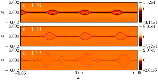
Figure 1: (Color online) Out-of-plane current density at different times shows fractal-like cascade to smaller scales via the plasmoid instability. First, the Sweet-Parker current sheet breaks up to form a chain of plamoids connected by secondary current sheets (top panel). Secondary current sheets are Sweet-Parker like, become unstable again, and generate the next batch of plasmoids (middle panel). This cascade leads to a hierarchy of plasmoids of various sizes (bottom panel). These snapshots present a small portion of the whole simulation box from a $S=10^{7}$ simulation. The reader is referred to Fig. 4 of Ref. Huang and Bhattacharjee (2010) for an illustration of the whole system.

After onset of the plasmoid instability, the reconnection layer changes to a chain of plasmoids connected by secondary current sheets that, in turn, may become unstable again. This process of cascading to smaller scales is reminiscent of fractals.Shibata and Tanuma (2001) If the large-scale configuration evolves slowly, eventually the reconnection layer will tend to a statistical steady state characterized by a hierarchical structure of plasmoids (see Fig. 1 for snapshots of the cascade). Two-dimensional numerical simulations show that reconnection rate becomes nearly independent of $S$ in this regime, with a value $\sim 0.01V_{A}B$.Bhattacharjee et al. (2009); Huang and Bhattacharjee (2010); Loureiro et al. (2012) The number of plasmoids $n_{p}$, the widths $\delta$ and lengths $l$ of secondary current sheets follow scaling relations $n_{p}\propto S$, $\delta\propto 1/S$, and $l\propto 1/S$.Huang and Bhattacharjee (2010) These scaling relations may be understood by assuming that all secondary current sheets are close to marginal stability. The rationale behind the assumption is as follows. Firstly, we note that cascade to smaller scales will stop if the local Lundquist number $lV_{A}/\eta$ of a secondary current sheet is smaller than $S_{c}$. Secondly, secondary current sheets typically get stretched and become longer over time due to gradient in the outflow, which on average increases from zero near the center to $\sim V_{A}$ near the ends of the reconnection layer. Thirdly, when the current sheet length $l$ becomes sufficiently long such that $lV_{A}/\eta>S_{c}$, the current sheet becomes unstable, new plasmoids are generated, and the fragmented current sheets become short again. Consequently, we expect the local Lundquist number $lV_{A}/\eta$ to stay close to $S_{c}$, i.e. $l\sim\eta S_{c}/V_{A}\sim LS_{c}/S$. The corresponding current sheet width $\delta\sim l/\sqrt{S_{c}}\sim LS_{c}^{1/2}/S$, and the number of plasmoids is estimated as $n_{p}\sim L/l\sim S/S_{c}$. Finally, reconnection rate can be estimated by $\eta J\sim\eta B/\delta\sim BV_{A}/\sqrt{S_{c}}\sim 10^{-2}V_{A}B$, which is independent of $S$. These scaling relations are consistent with the simulation results.

IV Statistical Distribution of Plasmoids

Statistical descriptions of plasmoids have drawn considerable interest in recent years, Fermo et al. (2010); Uzdensky et al. (2010); Fermo et al. (2011); Loureiro et al. (2012) partly due to the possible link between plasmoids and energetic particles.Drake et al. (2006); Chen et al. (2008b) The fractal-like fragmentation of current sheets suggests self-similarity across different scales,Shibata and Tanuma (2001) which often gives rise to power laws.Schroeder (1990) A recent heuristic argument by Uzdensky et al. suggests that if we consider the statistical distribution of the plasmoids in terms of their magnetic fluxes $\psi$, the distribution function $f(\psi)$ follows a power law $f(\psi)\sim\psi^{-2}$.Uzdensky et al. (2010) This result can be formally derived by adopting a model of plasmoid kinetics (similar to that given in Ref. Fermo et al. (2010)) and obtaining steady-state solutions of the plasmoid distribution.Huang and Bhattacharjee (2012)

The governing kinetic equation for the time evolution of $f(\psi)$ is written as

$$\frac{\partial f}{\partial t}+\alpha\frac{\partial f}{\partial\psi}=\zeta\delta(\psi)-\frac{fN}{\tau_{A}}-\frac{f}{\tau_{A}},$$ (3)

where $N(\psi)\equiv\int_{\psi}^{\infty}f(\psi^{\prime})d\psi^{\prime}$ is the cumulative distribution function, i.e. the number of plasmoids with fluxes larger than $\psi$. Several idealized assumptions have been made in writing Eq. (3). Firstly, the flux of a plasmoid grows due to reconnection in adjacent secondary current sheets. Following the assumption that all secondary current sheets are close to marginal stability, the flux of a plasmoid grows approximately at a constant rate $\alpha\sim BV_{A}/\sqrt{S_{c}}$. This gives the plasmoid growth term $\alpha\partial f/\partial\psi$ on the left hand side. Secondly, new plasmoids are created when a secondary current sheet becomes longer than the critical length for marginal stability. We assume that when new plasmoids are created, they contain zero flux; this is represented by the source term $\zeta\delta(\psi$), where $\delta(\psi)$ is the Dirac $\delta$-function, and $\zeta$ is the magnitude of the source. This source term sets the boundary condition for $f(\psi)$ at $\psi=0$. Thirdly, plasmoids disappear due to coalescence with larger plasmoids, which is assumed to be instantaneous. Assuming the characteristic relative velocity between plasmoids is of the order of $V_{A}$, the time scale of a plasmoid with flux $\psi$ to encounter a larger plasmoid is estimated as $\sim L/N(\psi)V_{A}\sim\tau_{A}/N(\psi)$. This gives the coalescence loss term $-fN/\tau_{A}$. Note that when two plasmoids coalesce, the flux of the merged plasmoid is equal to the larger of the two original fluxes.Fermo et al. (2010) Therefore, coalescence does not affect the value of $f$ at the larger of the two fluxes. Lastly, plasmoids are advected out from the reconnection layer with speeds $\sim V_{A}$ on a characteristic time scale $\tau_{A}$. This is represented by the advection loss term $-f/\tau_{A}$.

Exact steady-state solutions of Eq. (3) can be found analytically.Huang and Bhattacharjee (2012) However, for the discussion here it is instructive to consider approximate solutions in different regimes. At large $\psi$ when $N\ll 1$, the steady-state equation reduces to $\alpha\partial f/\partial\psi\simeq-f/\tau_{A}$. In this regime $f\sim\exp(-\psi/\alpha\tau_{A})$. On the other hand, when $N\gg 1$, the advection loss term is negligible, and we have $\alpha\partial f/\partial\psi\simeq-fN/\tau_{A}$. In this regime, $N\simeq 2\alpha\tau_{A}\psi^{-1}$ and $f=-\partial N/\partial\psi\simeq 2\alpha\tau_{A}\psi^{-2}$ is the solution. As such, the steady state solution admits both an exponential tail and a $f\sim\psi^{-2}$ power-law regime. The dominant loss mechanism in the former regime is advection, while it is coalescence in the latter. In other words, the plasmoids in the power-law regime must be deep in the hierarchy, whereas large plasmoids follow a distribution that falls off exponentially. Transition from the power-law regime to the exponential tail occurs when $N\simeq 1$, i.e. at $\psi\simeq 2\alpha\tau_{A}$. The distribution function $f(\psi)$ also deviates from the $\psi^{-2}$ power law in the small $\psi$ limit, otherwise the cumulative distribution function $N(\psi)$ will diverge as $\psi\to 0$. Because $N(\psi)\to n_{p}\sim S/S_{c}$ as $\psi\to 0$, the transition occurs when $2\alpha\tau_{A}\psi^{-1}\simeq n_{p}$, i.e. when $\psi\simeq 2\alpha\tau_{A}/n_{p}$. Therefore, the power law holds in the range $2\alpha\tau_{A}/n_{p}\ll\psi\ll 2\alpha\tau_{A}$, which becomes more extended for higher $S$.

This prediction of $f(\psi)\sim\psi^{-2}$ power-law distribution can be tested with numerical simulations. Figure 2 shows the cumulative distribution function $N(\psi)$ (panel (a)) and the distribution function $f(\psi)$ (panel (b)) from a $S=10^{7}$ simulation reported in Ref. Huang and Bhattacharjee (2012). The dataset was constituted of 30507 plasmoids collected from an ensemble of 521 snapshots during the quasi-steady phase with a cadence of 100 snapshots per $\tau_{A}$; an ensemble average was carried out for better statistics. The distribution function $f(\psi)$ exhibits an extended power-law regime; however, the power law is close to $f(\psi)\sim\psi^{-1}$ instead of $f(\psi)\sim\psi^{-2}$. The vertical dotted line denotes where $N(\psi)$ crosses $N=1$, indicating the switch of the dominant loss mechanism from coalescence to advection. From the above analysis, this switch of the dominant loss mechanism is responsible for the transition from a power-law distribution to an exponential falloff. And indeed, where $N(\psi)$ crosses $N=1$ approximately coincides with where the distribution function $f(\psi)$ starts to deviate from $f(\psi)\sim\psi^{-1}$ to a more rapid falloff. Incidentally, this rapidly falling tail was where Loureiro et al. attempted to fit with the $f(\psi)\sim\psi^{-2}$ power law.Loureiro et al. (2012) At smaller $\psi$, their reported distribution also appears to be consistent with $f(\psi)\sim\psi^{-1}$. Because our simulation only lasted a few $\tau_{A}$, the statistics in the large-$\psi$ regime is sufficiently uncertain that it is difficult to make a clear distinction between a $\psi^{-2}$ and an exponential falloff. Observationally, the distribution of the flux transfer events (FTEs) in the magnetopause from Cluster data, collected over a period of two years, appears to be consistent with an exponential tail.Fermo et al. (2011)

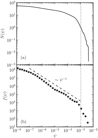
Figure 2: (a) Cumulative distribution function $N(\psi)$ and (b) distribution function $f(\psi)$ of plasmoids from a $S=10^{7}$ simulation. The vertical dotted line denotes where $N(\psi)=1$.

An alternative way to make a distinction between $\psi^{-1}$ and $\psi^{-2}$ distributions is to examine the distribution of the leading digit $d$ of the flux. (For example, if $\psi=2.35\times 10^{-5}$, then $d=2$.) Although the leading digit surely depends on the unit we use, the distribution of the leading digit will remain the same if the underlying distribution is a power law. For the $f(\psi)\sim\psi^{-1}$ distribution, the probability $P(d)$ of the leading digit $d$ follows Benford’s law $P(d)=\log_{10}(1+1/d)$.Benford (1938) On the other hand, the probability will be $P(d)=10/9d(d+1)$ if the distribution is $f(\psi)\sim\psi^{-2}$. Figure 3 shows the distribution of the leading digit, which is in good agreement with Benford’s law, but deviates significantly from the prediction corresponding to the distribution $f(\psi)\sim\psi^{-2}$. Because all plasmoids in the dataset, not just those in the power-law regime, are used in this analysis, the good agreement with Benford’s law reflects the fact that the majority of the plasmoids are in the $f(\psi)\sim\psi^{-1}$ power-law regime.

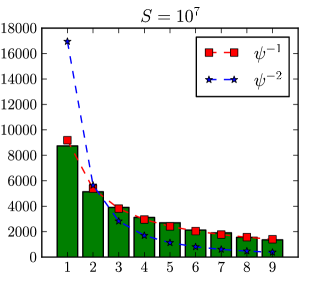
Figure 3: (Color online) The distribution of the leading digit of flux shows good agreement with Benford’s law (for $f(\psi)\sim\psi^{-1}$), but deviates significantly from the prediction based on $f(\psi)\sim\psi^{-2}$.

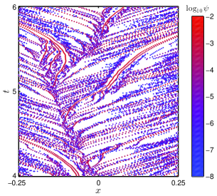
Figure 4: (Color online) Stack plot of plasmoid positions along the outflow direction $x$ during the period $t=4$ to $t=6$. Each dot represents a plasmoid, color coded according to its flux in logarithmic scale.

As we have discussed, the dominant balance in Eq. (3) leading to the $f(\psi)\sim\psi^{-2}$ solution is between the plasmoid growth term and the coalescence loss term, i.e. $\alpha\partial f/\partial\psi\simeq-fN/\tau_{A}$. A key assumption underlying the loss term $-fN/\tau_{A}$ is that the relative speeds of a plasmoid with respect to neighboring plasmoids larger than itself are of the order of $V_{A}$ and are uncorrelated to the flux of the plasmoid. However, that was found not to be the case when we examined the numerical data. Instead, the relative speeds between large plasmoids tend to be lower.Huang and Bhattacharjee (2012) Figure 4 shows the stack plot of plasmoid positions along the outflow direction $x$ over a period of $2\tau_{A}$, where each dot represents a plasmoid, color coded according to its flux in logarithmic scale. The stack plot has a tree-like structure, with branches that represent the trajectories of larger plasmoids shown on the red side of color scale. Those dots (or “leaves”) on the blue side of the color scale are mostly smaller plasmoids that do not show perceivable trajectories. We can clearly see that many branches are nearly parallel to their neighboring branches, indicating low relative speeds between large neighboring plasmoids.

This interesting phenomenon may be understood as follows. Roughly speaking, the flux of a plasmoid is proportional to its age because all plasmoids approximately grow at the same rate $\alpha$. Consequently, a plasmoid can become large only if it has not encountered plasmoids larger than itself for an extended period of time. Those plasmoids moving rapidly relative to their neighbors will encounter larger plasmoids and disappear easily, whereas those with small relative speeds are more likely to survive for a long time and become large. To incorporate this important effect, we have to consider a distribution function not only in flux, but also in velocity as well. Let $F(\psi,v)$ be the new distribution function, where $v$ is interpreted as the plasmoid velocity relative to the mean flow. We propose the following kinetic model for $F(\psi,v)$:

$$\partial_{t}F+\alpha\frac{\partial F}{\partial\psi}=\zeta\delta(\psi)h(v)-\frac{FH}{\tau_{A}}-\frac{F}{\tau_{A}},$$ (4)

where the function $H$ is defined as

$$H(\psi,v)=\int_{\psi}^{\infty}d\psi^{{}^{\prime}}\int_{-\infty}^{\infty}dv^{\prime}\frac{\left|v-v^{\prime}\right|}{V_{A}}F(\psi^{\prime},v^{\prime}),$$ (5)

and $h(v)$ is an arbitrary distribution function in velocity space when new plasmoids are generated. The distribution function $f(\psi)$ can be obtained by integrating $F(\psi,v)$ over velocity space. Eq. (4) differs from Eq. (3) in the coalescence loss term, where the relative speed $\left|v-v^{\prime}\right|$ between two plasmoids is taken into account in the integral operator of Eq. (5). If we replace $\left|v-v^{\prime}\right|$ in Eq. (5) by $V_{A}$, then Eq. (4) reduces to Eq. (3) after integrating over velocity space. By numerically solving for steady-state solutions of Eq. (4), we find that the distribution in the power-law regime is close to $f(\psi)\sim\psi^{-1}$, consistent with DNS results (see Figure 4 of Ref. Huang and Bhattacharjee (2012)). This conclusion does not appear to be sensitive to the specific form of $h(v)$, as long as $h(v)$ covers a broad range of $v$ (typically of the order of $V_{A}$).

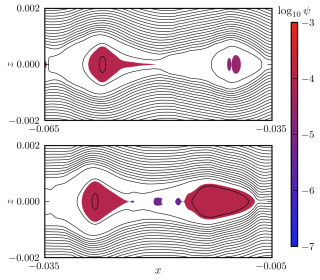
Figure 5: (Color online) Top: On the right hand side of the panel is an example of two partially merged plasmoids, both small in size. Bottom: When the merging is completed, they become a plasmoid much larger in extent. Also there are three new plasmoids generated in the middle. Contour lines represent magnetic field lines, and plasmoids are color coded with fluxes in logarithmic scale. Note that the two panels cover different ranges in the $x$ direction, because the whole structure is moving.

We caution the reader that although the heuristic argument in Sec. III and the kinetic model in this Section appear to account for the numerically observed scaling laws and plasmoid distributions, they are far from complete and satisfactory descriptions of the complex dynamics of a plasmoid-dominated reconnection layer. In particularly, a key building block of the present theory is the assumption that plasmoids are connected by marginally stable current sheets. That is clearly an oversimplification and does not appear to be always (and quite often not) the case upon close examination of simulation data;Huang and Bhattacharjee (2010) therefore, further exploration is warranted.Baty (2012) Some other potentially important effects are also omitted. For instance, plasmoids are treated as point “particles” and coalescence between them is assumed to occur instantaneously, whereas in reality larger plasmoids take longer to merge, and there can be bouncing (or sloshing) between them.Knoll and Chacón (2006); Karimabadi et al. (2011) Furthermore, the velocity $v$ relative to the mean flow is assumed to remain constant throughout the lifetime of a plasmoid, whereas in reality some variation is expected due to the complex dynamics between plasmoids.

The fact that plasmoids can be in a partially merged state can have significant effects on the statistical distribution,Loureiro et al. (2012) and this issue is further complicated by that there are different ways of identifying the extent of a plasmoid among researchers. In our diagnostics, plasmoids are extrema (O-points) of the flux function, which we solve as a primary variable in the simulation code. The extent of a plasmoid is determined by expanding the level set of the flux function from the extremum until it reaches a saddle point (X-point). Note that our convention differs from that adopted by Fermo et al. (see Figure 3 of Ref. Fermo et al. (2011)). Our method treats all plasmoids on equal footing, whereas that of Fermo et al. makes a distinction between the dominant and the lesser plasmoids for partially merged plasmoids. Although our method is mathematically unambiguous, it has a consequence that when two plasmoids are in the process of merging, both shrink in size until the merging is completed and a large plasmoid appears suddenly (Figure 5), whereas in the convention of Fermo et al. the lesser plasmoid shrinks in size and the dominant one keeps growing. This is a subtle point that merits further consideration if we apply the plasmoid distribution functions to the problem of particle energization.

V Roles of Plasmoid Instability in Onset of Collisionless Reconnection

Thus far, our discussion assumes that resistive MHD remains valid down to the smallest scales. This assumption is clearly questionable when current sheet widths reach kinetic scales, when two-fluid (Hall) and kinetic effects become important. Conventional wisdom had it that the onset of fast reconnection occurs when the Sweet-Parker width $\delta_{SP}$ is smaller than the ion inertial length $d_{i}$ (which should be replaced by the ion Larmor radius at the sound speed, $\rho_{s}$, if there is a strong guide field).Aydemir (1992); Ma and Bhattacharjee (1996); Dorelli and Birn (2003); Bhattacharjee (2004); Cassak et al. (2005, 2007) Because secondary current sheets can be much thinner than the Sweet-Parker width, the implication is that collisionless reconnection may set in even when the conventional criterion for onset is not met. This has been confirmed by several recent studies using fully kinetic Daughton et al. (2009) and Hall MHD Shepherd and Cassak (2010); Huang et al. (2011) models. Along with these studies, a practice has emerged of using phase diagrams to describe various possible “phases” of reconnection in the parameter space of $S$ and $\Lambda\equiv L/d_{i}$.Huang et al. (2011); Ji and Daughton (2011); Daughton and Roytershteyn (2012); Cassak and Drake (2013) Figure 6 shows our current rendition of the phase diagram, which is divided into seven regimes (including two history-dependent regimes), and five “phases”, that will be detailed as follows.

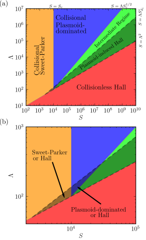
Figure 6: (Color online) (a) Phase diagram of magnetic reconnection that shows the five phases. (b) Expanded view about $S=10^{4}$ and $\Lambda=10^{2}$ shows two history-dependent regimes.

The collisionless Hall phase is realized when the conventional criterion for onset is satisfied, i.e. $\delta_{SP}<d_{i}$. In the parameter space of $S$ and $\Lambda$, that translates to $S>\Lambda^{2}$. This is the regime where reconnection dominated by collisionless effects will surely occur. In the region $S<\Lambda^{2}$, collisional Sweet-Parker reconnection can be realized if the current sheet is stable, i.e. when $S<S_{c}$. However, that is not always the case. An important phenomenon discovered by Cassak et al. is that reconnection is not uniquely determined by the parameters $S$ and $\Lambda$ alone; in a so called “bistable” region of the parameter space, both Sweet-Parker and Hall reconnection are possible, depending on the history in parameter space.Cassak et al. (2005, 2007, 2010); Sullivan et al. (2010) A useful parameter to discuss this hysteresis phenomenon is the Lundquist number based on $d_{i}$, defined as $S_{d_{i}}\equiv V_{A}d_{i}/\eta=S/\Lambda$, which characterizes the effect of resistivity on the $d_{i}$ scale. Disregarding the plasmoid instability, the condition for bistability may be expressed as $\Lambda>S_{d_{i}}>S_{d_{i}}^{c},$ or equivalently

$$\Lambda S_{d_{i}}^{c}<S<\Lambda^{2},$$ (6)

where $S_{d_{i}}^{c}$ is a critical value of $S_{d_{i}}$. The value of $S_{d_{i}}^{c}$ is found to be $\sim O(10^{2})$;Cassak et al. (2005); Huang et al. (2011) however, numerical evidence indicates that $S_{d_{i}}^{c}$ may increase with increasing $\Lambda$,Huang et al. (2011) although the precise scaling is not known. The parameter space defined by Eq. (6) is represented by the shaded region enclosed by dashed lines in Fig. 6, where we have assumed an arbitrary scaling just to show qualitatively the dependence of $S_{d_{i}}^{c}$ on $\Lambda$. The regime in the overlapping region defined by Eq. (6) and $S<S_{c}$ is the true “bistable” regime, where either collisionless Hall or collisional Sweet-Parker reconnection can be realized, depending on the history (see panel (b) of Fig. 6 for a zoom-in view).

When $S>S_{c}$, the Sweet-Parker current sheet is unstable. However, reconnection may remain collisional provided that secondary current sheet widths stay above the $d_{i}$ scale. Using the scaling estimate $\delta\sim LS_{c}^{1/2}/S$, the criterion is

$$S_{c}<S<\Lambda S_{c}^{1/2},$$ (7)

which defines the collisional plasmoid-dominated phase. Note that the there is an overlapping region defined by Eq. (6) and Eq. (7) together (again see panel (b) of Fig. 6 for a zoom-in view). That suggests there may exist a history-dependent regime where both collisionless Hall and collisional plasmoid-dominated reconnection can be realized. Although this regime has not been demonstrated in simulation, it remains an interesting possibility.

The region defined by $\Lambda S_{c}^{1/2}<S<\Lambda^{2}$ is where secondary current sheets can reach the $d_{i}$ scale. Where this region overlaps the “bistable” region defined by Eq. (6) is the “plasmoid-induced Hall” phase. Although this regime is supposed to be bistable according to Eq. (6), Sweet-Parker reconnection ceases to exist due to the plasmoid instability, and collisionless Hall reconnection is the only possibility. The only difference between the “plasmoid-induced Hall” regime and the “collisionless Hall” regime is the process of reaching collisionless Hall reconnection. In the former, onset of Hall reconnection is proceeded by cascading to smaller scales induced by plasmoids, whereas in the latter the primary current sheet will reach the kinetic scales and immediately trigger the onset of Hall reconnection.

The region defined by $\Lambda S_{c}^{1/2}<S<\Lambda S_{d_{i}}^{c}$ is the “intermediate regime” where the system alternates between collisional and collisionless reconnection. On the one hand, secondary current sheets can reach the $d_{i}$ scale and trigger onset of Hall reconnection. On the other hand, after onset of Hall reconnection the system cannot settle down to a localized Hall reconnection geometry because it is physically unrealizable. This regime has been realized in a large scale Hall MHD simulation, where the current sheet becomes extended again after onset of Hall reconnection. That leads to formation of new plasmoids and another onset of Hall reconnection.Huang et al. (2011)

From what we have learned so far, among these phases, the collisional plasmoid-dominated regime gives the slowest reconnection rate, which is approximately $0.01V_{A}B$. The collisional Sweet-Parker regime yields faster reconnection, because resistivity is high. Collisionless Hall reconnection rate typically attains a maximum value $\sim 0.1V_{A}B$, whereas in the intermediate regime the reconnection rate can oscillate between $0.01V_{A}B$ and $0.1V_{A}B$.

There have been different renditions of phase diagrams proposed in recent literature. Huang et al. (2011); Ji and Daughton (2011); Daughton and Roytershteyn (2012); Cassak and Drake (2013) All of them share a great similarity, with some minor differences. Because the parameter space has not been systematically explored, these phase diagrams are necessarily speculative to some extent. Nonetheless, they can serve as a good frame of reference to explore large scale magnetic reconnection, either in choosing simulation parameters Huang et al. (2011) or in planning for future experiments.Ji and Daughton (2011) One should bear in mind that the border lines between different phases are not ironclad, because there is no clear-cut value of $S_{c}$. Furthermore, secondary current sheet widths can deviate from the estimated value $\delta\sim LS_{c}^{1/2}/S$. Finally, both $S_{c}$ and $\delta$ can be affected by Hall effects.Baalrud et al. (2011) More caveats in applying the phase diagrams are discussed in Ref. Cassak and Drake (2013), and a compilation of parameters for various astrophysical, space, and laboratory plasmas can be found in Ref. Ji and Daughton (2011).

VI Discussion and Future Challenges

Although significant advances have been made in recent years on large scale, high-Lundquist-number reconnection, where plasmoids play important roles, many questions remain open. The results presented here are based on 2D studies. To what extent do these 2D results carry over to 3D geometry, where oblique tearing modes have been shown to play an important role?Daughton et al. (2011); Baalrud et al. (2012) The relationship between plasmoid-dominated reconnection and turbulent reconnectionLazarian and Vishniac (1999); Kowal et al. (2009); Eyink et al. (2011); Lazarian et al. (2012) is another issue that needs further investigation. What are their similarities and differences? Will the interaction between overlapping oblique modes in 3D lead to self-generated turbulence and further blur the line between the two?

How do global conditions affect the plasmoid instability and magnetic reconnection in general also needs further assessment. One of the most important results from recent 2D studies is that reconnection rate cannot be significantly slower than $10^{-2}V_{A}B$, therefore is always fast (although this has only been tested up to $S\sim 10^{7}$). This conclusion poses new challenges to theories of solar flares that assume the existence of slow reconnection.Uzdensky (2007a, b); Cassak et al. (2008); Cassak and Shay (2012); Cassak and Drake (2013) However, these studies were done in simple 2D configurations, and it is not clear whether the results can be directly applied to solar corona, where the line-tying effect is thought to play an important role.Gibons and Spicer (1981); Hood (1986, 1992); Longcope and Strauss (1994) Line-tying is known to have stabilizing effect on tearing instability Delzanno and Finn (2008); Huang and Zweibel (2009) and smoothing effect on current sheets.Evstatiev et al. (2006); Huang et al. (2006, 2010) Both effects could significantly affect the plasmoid instability. Although line-tying has been employed in the lower boundary of some recent 2D simulations of the plasmoid instability in coronal current sheets, Bárta et al. (2011b); Shen et al. (2011); Mei et al. (2012) these studies are limited to anti-parallel reconnection, where line-tying stabilization is not effective. Line-tying stabilization of the tearing instability is more effective for component reconnection, with the guide field line-tied to the boundary. Therefore, to study the effects of line-tying on the plasmoid instability, 3D simulations will be needed.

Even in 2D systems, the current understanding is far from complete. The parameter space needs to be systematically explored with higher Lundquist number and larger system size than that have been achieved, to test the proposed phase diagrams. The kinetic model of plasmoid distribution can be further improved by including other coarse-graining variables in addition to $\psi$ and $v$, and the distribution of plasmoids in collisionless regime needs to be further studied.