How to test for mass degenerate Higgs resonances

Abstract

The Higgs-like signal observed at the LHC could be due to several mass degenerate resonances. We show that the number of resonances is related to the rank of a “production and decay” matrix, $R_{if}$. Each entry in this matrix contains the observed rate in a particular production mode $i$ and final state $f$. In the case of $N$ non-interfering resonances, the rank of $R$ is, at most, $N$. If interference plays a role, the maximum rank is generically $N^{2}$, or with a universal phase, $N(N+1)/2$. As an illustration we use the present experimental data to constrain the rank of the corresponding matrix. We estimate the LHC reach of probing two and three resonances under various speculations on future measurements and uncertainties.

I Introduction

At present there is clear evidence for a new boson at the Large Hadron Collider (LHC) with a mass of about 126 GeV :2012gk ; :2012gu . In this paper we are interested in the possibility that the signal is due to two or more mass degenerate states. We are especially interested in the question whether one can tell experimentally if there are more resonances, and perhaps even constrain their number, without actually resolving the resonant peaks. That is, we are interested in the case that the resonances are mass degenerate to better than the experimental resolution.

So far, the observed rates $R_{if}$ of the 126 GeV resonance have been consistent with the Standard Model (SM) Higgs boson, although their central values do exhibit ${\cal O}(1)$ deviations. Here $i$ runs over the production modes: gluon fusion, vector boson fusion, associated production, while the final states $f$ are $\gamma\gamma$, $\tau\tau$, etc. By itself, any deviation from the SM prediction in one element of $R_{if}$ can be explained by some kind of a new physics scenario with one resonance. Some patterns of deviations in $R_{if}$, however, are bound to be inconsistent with the hypothesis of a single resonance, even if one allows for non-SM couplings. This is easily understood using a counting argument. We denote the number of observed production (decay) modes by $n_{i}$ $(n_{f})$. Assuming there is a single resonance, the unknowns are the $n_{i}$ cross sections $\{\sigma_{i}\}$ and $n_{f}$ branching ratios $\{B_{f}\}$. The number of observables is $n_{i}n_{f}$, which are all the entires in $R_{if}$. Thus, the set of equations one has to solve is

$$\sigma_{i}B_{f}=R_{if}.$$ (1)

In this system of equations the number of unknowns, $n_{i}+n_{f}$, can be less than the number of observables, $n_{i}n_{f}$. With enough measurements, this may lead to a system of equations which is overdetermined and potentially inconsistent. Such inconsistency cannot be removed by any type of new physics that affects only the production or decay of a single resonance. We would then be forced to abandon the single resonance hypothesis and conclude that there are more resonances.

The idea of using such inconsistency for detecting two resonances has been pioneered in Ref. Gunion:2012he , where the authors used ratios of the form $R_{ia}/R_{ib}$. For fixed $a$ and $b$ these ratios are independent of $i$, if there is only one resonance. This can then be used to test for the existence of more than one resonance (invoking two resonances to enhance the diphoton rate has been mentioned recently in Gunion:2012gc for the NMSSM and in Ferreira:2012nv ; Drozd:2012vf for two Higgs doublet models). In this paper we generalize the condition above to including any number of resonances, as well as interference effects. Alternatively, the existence of extra resonances may be directly probed using line shapes, see e.g. Ellis:2005fp ; Ellis:2004fs .

Assuming no interference between the resonances we find that ${{{\rm rank}(}R)}$, the rank of the signal matrix $R_{if}$, constitutes a lower bound on the number of resonances required to explain the data. For interfering resonances we find, on the other hand, that this lower bound is relaxed to the integer that is greater or equal to $\sqrt{{{{\rm rank}(}R)}}$ in the most general case or to $\big{(}\sqrt{1+8\,{{{\rm rank}(}R)}}-1\big{)}/2$ if a universal phase (i.e. independent of $i$ and $f$) is assumed. It follows that if ${{{\rm rank}(}R)}\geq 2$, there must be at least two resonances, whereas if ${{{\rm rank}(}R)}\geq 3$, the resonances must interfere, or there must be at least three of them.

II General discussion

We begin by recalling a few useful mathematical relations. Consider two sets of vectors in $\mathbb{C}^{N}$

$$\mbox{\boldmath${u}$}^{r}\equiv\left(u_{1}^{r},\ldots,u_{N}^{r}\right),\qquad\mbox{\boldmath${v}$}^{r}\equiv\left(v_{1}^{r},\ldots,v_{N}^{r}\right),$$ (2)

where $r=1,\dots,n$ and we assume $N\gg n$. We define two $N\times N$ matrices whose elements are

$$A_{ij}=\sum_{r=1}^{n}\left|u_{i}^{r}\,v_{j}^{r}\right|^{2},\qquad B_{ij}=\left|\sum_{r=1}^{n}u_{i}^{r}\,v_{j}^{r}\right|^{2}.$$ (3)

Then one can prove that generically,

$${{\rm rank}\,}A=n,\qquad{{\rm rank}\,}B=n^{2}.$$ (4)

When the phase between $u_{i}^{r}v_{j}^{r}$ and $u_{i}^{r^{\prime}}v_{j}^{r^{\prime}}$ is independent of $i,j$, the above results are modified such that

$${{\rm rank}\,}A=n,\qquad{{\rm rank}\,}B=\frac{n(n+1)}{2}.$$ (5)

Note that the condition leading to (5) is satisfied when the vectors are real.

More generally, $u$ and $v$ can have different dimensions, and we may have cancellations if the elements are not generic. Thus a more general result is to treat the r.h.s. of the relations in Eqs. (4) and (5) and as an upper bound on the corresponding ranks. Of course, the rank is also bounded by $N$. Equipped with these results we now return to physics.

Suppose there exist $n_{r}>1$ resonances $\{\phi_{1},\cdots,\phi_{n_{r}}\}$ all with masses close enough so that the experimental resolution is not sufficient to resolve them. If the masses of different resonances are split by much more than their respective decay widths, interference effects are highly suppressed and can be neglected. The signal strengths $R_{if}$ are then given by

$$R_{if}=\sum_{r=1}^{n_{r}}\hat{\sigma}_{i}^{r}\hat{B}_{f}^{r}\equiv\mbox{\boldmath${\hat{\sigma}}$}_{i}\cdot\mbox{\boldmath${\hat{B}}$}_{f},$$ (6)

where the production cross sections $\hat{\sigma}_{i}^{r}\equiv\sigma_{i}^{r}/\sigma_{i}^{\rm SM}$ and branching ratios $\hat{B}_{i}^{r}\equiv B_{i}^{r}/B_{i}^{\rm SM}$ for each resonance $r$ are normalized to the SM values. The sum in Eq. (6) runs over the degenerate resonances $r=1,\dots,n_{r}$. Using Eq. (4) we see that

$$n_{r}\geq{{{\rm rank}(}R)}.$$ (7)

Namely, if one is able to measure ${{{\rm rank}(}R)}$, it would imply a lower bound on the number of resonances. Recall that the rank of a matrix $R_{if}$ is equal to the number of linearly independent rows or columns, and may be obtained, e.g., using singular value decomposition (SVD), where the number of nonzero singular values equals ${{{\rm rank}(}R)}$.

If the decay widths are larger than the mass splittings between resonances, interference effects may be important. For instance, for perfectly overlapping resonances,

$$R_{if}=\left|\sum_{r=1}^{n_{r}}A_{i}^{r}A_{f}^{r}\right|^{2}\equiv\left|\mbox{\boldmath${A}$}_{i}\cdot\mbox{\boldmath${A}$}_{f}\right|^{2},$$ (8)

where $A_{i}^{r}$ and $A_{f}^{r}$ are the properly normalized amplitudes for the production and decay of the resonance $r$, such that $\hat{\sigma}_{i}^{r}=|A_{i}^{r}|^{2}$ and $\hat{B}_{f}^{r}=|A_{f}^{r}|^{2}$. In contrast to the non interfering case, the elements of $R_{if}$ are no longer given by a sum of positive terms, and cancellations may occur. Thus, small entries in $R_{if}$ are possible, even when $\sigma_{i}^{r}$ and $B_{f}^{r}$ are large, providing more model building freedom.

Moreover, interference affects the relation between $n_{r}$ and the rank of $R$. Indeed, applying Eq. (4) to Eq. (8) results in

$${{{\rm rank}(}R)}\leq n_{r}^{2}\quad\Rightarrow\quad n_{r}\geq\sqrt{{{{\rm rank}(}R)}}.$$ (9)

In the case of a universal phase, i.e., a phase which depends only on the resonance $\phi_{r}$ but not on the individual production ($i$) and decay ($f$) mechanisms, we can apply Eq. (5) to Eq. (8) and obtain

$${{{\rm rank}(}R)}\leq\frac{n_{r}(n_{r}+1)}{2}.$$ (10)

Solving for $n_{r}$ we obtain the lower bound

$$n_{r}\geq\frac{1}{2}\big{(}\sqrt{1+8\,{{{\rm rank}(}R)}}-1\big{)}.$$ (11)

This occurs, for example, in the case where CP is conserved and the contributions of light fields running in the gluon fusion and diphoton loops can be neglected. CP-even (“strong”) phases may come from three sources. The first is the inherent Breit-Wigner $s$-dependence of the decay amplitude, which is universal since it depends only on the decay width. The second is rescattering of final states, which is not universal but can be neglected if we assume perturbativity. A third possible source of CP-even phase is when the leading diagram is a loop process mediated by light fields running in the loop. Then the imaginary component of the leading diagram may be sizable by virtue of the optical theorem, resulting in an ${\cal O}(1)$ non-universal phase. This may occur, e.g., in certain large $\tan\beta$ scenarios, where gluon fusion or diphoton decay are mediated by the $b$ quarks and $\tau$ leptons.

It follows that any data which can be explained using $n_{r}$ non-interfering resonances may possibly also be explained with fewer interfering ones. For example, if the data satisfies ${{{\rm rank}(}R)}=3$, there must be at least 2 interfering resonances, or 3 resonances without interference among them. In the case where the data suggest ${{{\rm rank}(}R)}=4$, there must be at least 2 interfering resonances or 3 interfering resonances with universal phases or 4 non interfering ones.

We conclude this section with a few remarks.

1. First we comment on the transition between the interfering and non-interfering case. This transition must be smooth, yet our result above seems discontinuous. This may be understood as follows. When interference is taken into account, the extra non vanishing singular values of the matrix $R$ are proportional to the size of the interference term. When the resonances are far apart, their interference is negligible and proportional to their overlap, and the singular values approach zero. For example, consider two resonances with equal width $\Gamma$ and mass difference $\Delta m$. In this case, we expect two singular values to be similar, while the third one is suppressed by the overlap. In the Breit-Wigner approximation, it is given by $(2\Gamma/\Delta m)^{2}$, although realistic profiles may deviate from the Breit-Wigner curve at their tails.

2. In case of universal phases, the interference can still increase the rank of $R$, however, the resulting matrix is not generic. For example, when all the amplitudes are real, the matrix $\sqrt{R_{ij}}$ has the same rank as that of $R_{ij}$ in the non interfering case.

3. In all of the above, we have ignored effects of interference between the signal and the SM background. Such effects were studied, for example, in the case of $gg\to H\to\gamma\gamma$ Dixon:2003yb ; Martin:2012xc . While this effect can be experimentally taken into account in the SM, it cannot be done model independently. Yet, taking the SM as a benchmark, we may estimate the effect to be small enough, and ignore it. It may become an issue in the future.

III Numerical Examples

We discuss next a few concrete numerical examples, starting with the information that can be extracted already with present experimental precision and then contemplate projections to the future. The current status of the signal strength matrix $R_{if}$ is given in Table 1, where we have averaged the experimental results from ATLAS and CMS.

prod.$\backslash$decay	$\gamma\gamma$	$WW^{*}$	$\tau\bar{\tau}$	$ZZ^{*}$	$b\bar{b}$
$gg$	$1.6\pm 0.35$ ATLASgamma ; CMScomb	$0.8\pm 0.3$ ATLAScomb ; CMScomb	$1.2\pm 0.8$ ATLAStautau ; CMStautau	$1.0\pm 0.3$ ATLASZZ	$-$
VBF	$2.1\pm 0.9$ ATLASgamma ; CMScomb	$-0.2\pm 0.6$ ATLAScomb ; CMScomb	$0.3\pm 0.7$ ATLAStautau ; CMStautau	$-$	$-$
$VH$	$1.9\pm 2.6$ ATLASgamma	$-0.3\pm 2.1$ CMScomb	$1.0\pm 1.8$ CMStautau	$-$	$0.8\pm 0.6$ ATLASbbbar
$t\bar{t}h$	$-$	$-$	$-$	$-$	$<3.8$ CMSttbar

Table 1: The experimental values of signal strengths, $R_{if}$, for several production modes (listed in the first column) and different final states (listed in the first row) obtained by naively averaging ATLAS and CMS results with statistical and systematic errors added in quadrature and neglecting correlations.

In general, the signal strengths $R_{if}$ are measured with finite precision $\delta R_{if}$. We simplify the discussion by neglecting correlations between different channels, cross contaminations and other systematic errors. For instance, depending on the cuts, some of the $gg$ signal can appear in the vector boson fusion (VBF) production channel, as is the case in $h\to\gamma\gamma$. These effects were partially taken into account in Table 1, e.g. for the $\gamma\gamma$ final state. We also assume that the acceptances in the NP models are similar to those of a SM Higgs boson. This may be simply realized by assuming that different resonances are described by the same low energy effective Lagrangian as the SM Higgs Espinosa:2012ir ; Azatov:2012bz ; Azatov:2012qz ; Carmi:2012yp . While these approximations suffice at present precision, we emphasize that these effects can be important and there is no reason for them not to be included in a full-fledged analysis.

To constrain the number of resonances, we are interested in the statistical properties of the hypothesis that ${{{\rm rank}(}R)}\geq r$. Note that one can only put a lower bound on the rank since including experimental errors generally increase it. Finding the significances for each possible $r$ may be done in a number of ways. Below we discuss two of these, but there are many other possibilities. The best approach then depends on the particular situation. Depending on the exact situation, one way may be better than another.

III.1 Using Singular Value Decomposition

Obtaining the rank of $R$ may be done most generally by using singular value decomposition (SVD),

$$R=USV^{T},$$ (12)

where $U$ and $V$ are orthogonal matrices with dimensions $n_{i}$ and $n_{f}$ respectively, and $S$ is a rectangular ($n_{i}\times n_{f}$) diagonal matrix. The diagonal elements of $S$ are the singular values, $\lambda_{i}\equiv S_{ii}$ (no summation), and may be obtained by diagonalizing $RR^{T}$ (using $U$) or $R^{T}R$ (using $V$). By definition $\lambda_{i}$ are non-negative, which can always be accomplished by appropriate redefinition of $U$ and $V$. It is convenient to define $S$, $U$ and $V$, such that the singular values are ordered with $\lambda_{1}$ the largest. The rank of an exactly known matrix is given by the number of nonzero singular values $N(\lambda_{i}\neq 0)$. Since in our case the matrix $R$ is only known to a certain precision, these singular values have distributions induced by the uncertainties of the matrix elements. To obtain a statistical test of ${{{\rm rank}(}R)}$ we follow the procedure of Kleibergen:2006 . We split $U$, $S$ and $V$ into the block matrices

$$U=\begin{pmatrix}U_{r\times r}&\dots\\ \dots&\tilde{U}\end{pmatrix},\qquad S=\begin{pmatrix}S_{r\times r}&0\\ 0&\tilde{S}\end{pmatrix},\qquad V=\begin{pmatrix}V_{r\times r}&\dots\\ \dots&\tilde{V}\end{pmatrix},$$ (13)

where $\tilde{U}$ is an $(n_{i}-r)\times(n_{i}-r)$ square matrix, $\tilde{S}$ an $(n_{i}-r)\times(n_{f}-r)$ rectangular diagonal matrix, and $\tilde{V}$ and $(n_{f}-r)\times(n_{f}-r)$ square matrix. We then construct

$$\Lambda_{r}\equiv\tilde{U}\tilde{S}\tilde{V}^{T},$$ (14)

which is an $(n_{i}-r)\times(n_{f}-r)$ matrix that is zero if the singular values are zero. (Note that we differ in the normalization of $\Lambda_{r}$ from Kleibergen:2006 .) We can then test whether singular values are consistent with zero simply by asking whether $\Lambda_{r}$ is consistent with zero. We neglect correlations and assume that the errors for the matrix elements of $\Lambda_{r}$ are Gaussian, which we denote by $\sigma[(\Lambda_{r})_{ij}]$. We then define

$$\chi^{2}(\Lambda_{r})\equiv\sum_{i,j}\left(\frac{(\Lambda_{r})_{ij}}{\sigma[(\Lambda_{r})_{ij}]}\right)^{2},$$ (15)

which approaches the $\chi^{2}$ distribution for $(n_{i}-r)\times(n_{f}-r)$ degrees of freedom in the large statistics limit. While we do not propagate the correlations, one could easily modify the above definition of $\chi^{2}(\Lambda_{r})$ to take into account the correlations. On average we expect $\chi^{2}(\Lambda_{r})=(n_{i}-r)\times(n_{f}-r)$. Much higher values would correspond to $\Lambda_{r}$ significantly nonzero, with CL obtained from $\chi^{2}$ distribution, signaling that the rank of the matrix $R$ is at least $r+1$. The advantage of working with $\Lambda_{r}$ instead of with singular values is that the entries of $\Lambda_{r}$ are not bound to be non-negative (cf. Fig. 1) so that it is easier to devise such a simple $\chi^{2}$ test.

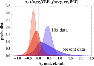
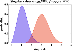
Figure 1: Left: The probability distributions for the $(\Lambda_{1})_{11}$ (blue) and $(\Lambda_{1})_{12}$ (red) entries with present data and for $10\times$ more data assuming present central values and the dominance of statistical errors. The $R_{if}$ matrix has entries from $i=\{gg,$VBF} and $f=\{\gamma\gamma,\tau\tau,WW\}$ channels. Right: The probability distributions for the two singular values of the $2\times 3$ $R_{if}$ matrix.

Next, we apply the above method to the data. The largest matrix $R_{if}$ that we can form using present measurements is $3\times 3$, with $i=\{gg,$VBF,VH} and $f=\{\gamma\gamma,\tau\tau,WW\}$ collected in Table 1. Since the last row is least well measured we choose to use the $2\times 3$ rectangular submatrix $i=\{gg,$VBF} and $f=\{\gamma\gamma,\tau\tau,WW\}$ for the numerical examples (we will return to the $3\times 3$ case below). The most obvious test is for ${{{\rm rank}(}R)}\geq 1$, choosing $r=0$ in (13). This means that $\Lambda_{0}=R$. Neglecting correlations we have $\chi^{2}(\Lambda_{0})=36.1$ for $6$ d.o.f., which corresponds to a probability $1-{\rm CL}=3\cdot 10^{-6}$ that this is just a statistical fluctuation. The signal significance is $4.7\sigma$ and we confirm the hypothesis of at least one resonance.

Testing whether ${{{\rm rank}(}R)}=2$ we take $r=1$, so that $\Lambda_{1}$ is a $1\times 2$ matrix. The probability distributions for the two entries in $\Lambda_{1}$ are shown in Fig. 1 (left) and were obtained from simple Monte Carlo with $10^{6}$ iterations assuming Gaussian errors for the $R_{if}$ matrix elements. This gives $\chi^{2}(\Lambda_{1})=0.8$ which is not statistically significant for 2 d.o.f. as it corresponds to $0.4\sigma$ signal significance. That is, with the current data we cannot test for more than one resonance. With ten times more data, however, assuming the same central values and scaling of errors as $1/\sqrt{L}$, one would obtain a signal for ${{{\rm rank}(}R)}=2$ with $3.9\sigma$ significance. While this is just a very crude estimate, we conclude that with roughly an order of magnitude more data we will be able to probe for a rank two matrix.

III.2 Using The Determinant

While the method described above is very general, in some cases we can devise simpler tests. When $R$ is a square block matrix ($n_{i}=n_{f}=n$) one can check if ${\det R}$ is significantly nonzero, which would imply that the rank of $R$ is $n$. For $2\times 2$ blocks (i.e., $n_{i}=n_{f}=2$), the determinant already contains the maximal information available on the number of resonances, since ${\det R}=0$ implies that one resonance suffices, while a ${\det R}\neq 0$ implies $n_{r}\geq 2$. For larger square blocks, however, the determinant can only distinguish the $n_{r}\geq n$ case against $n_{r}<n$. We will now give examples for both $2\times 2$ and $3\times 3$ blocks. While the former probes two resonances, the latter allows to probe three resonances and interference.

First, consider the two $2\times 2$ sub-matrices $R^{A}=(\{gg,\mbox{VBF}\},\{\gamma\gamma,\tau\tau\})$ and $R^{B}=(\{gg,\mbox{VBF}\},\{\gamma\gamma,WW\})$. The SM is excluded if any $R_{i,f}\neq 1$. The single resonance hypothesis is excluded if ${\det R}^{A}\neq 0$ or ${\det R}^{B}\neq 0$. When formulated in term of the ratios

$$r_{1}\equiv\frac{R_{{\rm VBF},WW}}{R_{{\rm VBF},\gamma\gamma}},\qquad r_{2}\equiv\frac{R_{gg,WW}}{R_{gg,\gamma\gamma}},\qquad r_{3}\equiv\frac{R_{{\rm VBF},\tau\tau}}{R_{{\rm VBF},\gamma\gamma}},\qquad r_{4}\equiv\frac{R_{gg,\tau\tau}}{R_{gg,\gamma\gamma}},$$ (16)

these inequalities become $r_{1}\neq r_{2}$ or $r_{3}\neq r_{4}$. Ratios such as above have been considered in Gunion:2012he , and have the virtue that certain systematic errors cancel (this has been recently pointed out also in Low:2012rj ). As an example, consider a situation in which all the rates remain at their current central values with much reduced errors, except $R_{{\rm VBF}\,,WW}$, which we take to be small instead of the current negative value:

$$R_{gg\,,\gamma\gamma}=1.6,\qquad R_{{\rm VBF}\,,\gamma\gamma}=2.1,\qquad R_{gg\,,WW}=0.8,\qquad R_{{\rm VBF}\,,WW}=0.1.$$ (17)

Interpreting such hypothetical results as coming from a single on-shell particle is inconsistent, since the resulting signal matrix has nonzero determinant, ${\det R}\neq 0$. In terms of ratios, this fact is evident in the inequality of the ratios

$$\frac{R_{{\rm VBF}\,,WW}}{R_{{\rm VBF}\,,\gamma\gamma}}=0.048,\qquad\frac{R_{gg\,,WW}}{R_{gg\,,\gamma\gamma}}=0.5,$$ (18)

while for a single resonance the two ratios would be identical and equal to $\hat{B}r_{WW}/\hat{B}r_{\gamma\gamma}$. If this inequality becomes certain in the future, it will therefore point to ${{{\rm rank}(}R)}=2$, implying the existence of at least two mass degenerate resonances, $\phi_{1}$ and $\phi_{2}$. Such hypothetical result could be explained, for example if $\phi_{1}$ does not couple to $W$ bosons while $\phi_{2}$ does not couple to photons. Note that since we have assumed low $R_{{\rm VBF},WW}$, if the resonances do not interfere, some of the parameters need to be suppressed, for example, the “Higgs” coupling to $WW$. This is because in that case the $R_{if}$ values are sums of positive numbers. In contrast, no such suppression is needed for interfering resonances where the suppression can come from negative interference. This provides more model building freedom.

A more realistic discussion includes experimental errors, where one tests for a statistically significant deviation from ${\det R}=0$. In Fig. 2, we show contours of the integrated luminosity required to exclude at $3\sigma$ the SM (blue) or the single resonance hypothesis (green), in the $(r_{1},r_{2})$ and $(r_{3},r_{4})$ planes. In the extrapolation we assume statistical scaling of errors, that is $\propto 1/\sqrt{L}$, and central values taken from Table 1. We find that if the current central values remain where they are now, then ${\mathcal{O}}(300\text{fb}^{-1})$ at LHC 14TeV would suffice to exclude at $3\sigma$ the single resonance hypothesis.

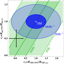
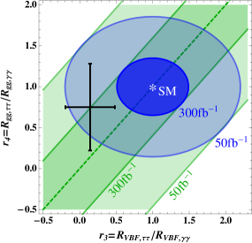
Figure 2: Contours of constant integrated luminosity at LHC 14 TeV required to exclude at $3\sigma$ the SM (the single resonance hypothesis) if the measurement is within blue (green) regions in the $(r_{1},r_{2})$ plane (left) and in the $(r_{3},r_{4})$ plane (right). We have assumed statistical scaling of errors, while present $1\sigma$ measurements are denoted with black error bars. The 14 TeV run projections were obtained by rescaling the current $7+8$ TeV errors with the increase in the higgs production cross section xsecs to reflect the gain in statistics.

Finally, we discuss the possibility of testing for rank 3. Note that this is not only a generalization from 2 resonances to 3, it is also the lowest possible rank which can probe interference. As an example we test for rank 3 using ${\det R}\neq 0$ test for $n=3$. This distinguishes between ${{{\rm rank}(}R)}=3$ and ${{{\rm rank}(}R)}=1,2$ cases. The ${{{\rm rank}(}R)}=1$ and ${{{\rm rank}(}R)}=2$ cases may be resolved using SVD, as discussed in Eqs. (12)-(15). For inputs we use the $(\{gg,\mbox{VBF},VH\},\{\gamma\gamma,WW,\tau\tau\})$ block in Table 1.

First, consider an idealized future scenario, where all the central values are as in Table 1, except the negative ones, which we take to be $+0.1$, for illustration purposes. The relevant matrix has rank 3, and can be decomposed as usual using three non-overlapping resonances. The same matrix can also result from 2 resonances, provided they interfere (cf. Sec. II). For example, the two resonances may have the following amplitudes,

$$\mbox{\boldmath${A}$}_{gg} = \left(1,0.458\,e^{0.5i}\right),\,\mbox{\boldmath${A}$}_{\rm VBF}=\left(0.673\,e^{-1.5i},1.088\,e^{0.4i}\right),\,\mbox{\boldmath${A}$}_{VH}=\left(1.11\,e^{0.05i},1.277\,e^{2i}\right),$$

$$\mbox{\boldmath${A}$}_{\gamma\gamma} = \left(1,1.95\,e^{1.2i}\right),\,\mbox{\boldmath${A}$}_{WW^{*}}=\left(0.9\,e^{1.9i},0.69\,e^{-3.1i}\right),\,\mbox{\boldmath${A}$}_{\tau\bar{\tau}}=\left(1.1\,e^{0.4i},0.17\,e^{1.6i}\right).$$ (19)

Note that this example requires a non-universal phase. As we mentioned before, an example with a universal phase does not always exist. However, often a universal phase model can produce a matrix that is in the vicinity of the one that is needed. Thus, it is not clear how much data one would need in order to probe non-universal phases.

We are now ready to discuss the more realistic case with finite statistics. We show the projected sensitivity in Fig. 3(left), assuming statistical scaling of errors, and assuming the cross sections scale with center of mass energy as they do in the SM. In this case ${\mathcal{O}}(300\text{fb}^{-1})$ at LHC 14 TeV are needed for $3\sigma$ evidence of two resonance case using the ${{{\rm rank}(}R)}=2$ test described above. We estimate that ${\mathcal{O}}(2000\text{fb}^{-1})$ at LHC 14 TeV are needed for $3\sigma$ evidence of three overlapping resonances using the test that $\det R\neq 0$. It is important to note that all these estimates crucially depend on the input parameters and ${\mathcal{O}}(1)$ change in the central value of just one parameter can lead to a factor of few smaller required luminosities. Therefore, in the right panel we show a plot where the central values are allowed to vary. Contours of constant luminosity are shown where the significance for discovering 3 non-interfering or 2 interfering resonances (${\det R}\neq 0$) reaches $3\sigma$. The error has been propagated linearly by expanding the determinant. While this is clearly not adequate for large relative errors, it provides a rough estimate for the significance.

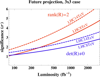
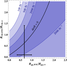
Figure 3: Left: The projected significance for a discovery of 3 (2) overlapping resonances using $3\times 3$ $R$ matrix (see text) using the ${\det R}\neq 0$ (${{{\rm rank}(}R)}\geq 2$) tests are shown with solid and dashed blue (red) lines for LHC at 8TeV and LHC at 14 TeV, respectively, as a function of integrated luminosity. Right: Integrated luminosity at 14 TeV LHC required to probe 3 non-interfering or 2 interfering resonances with $3\sigma$ significance as a function of the ratios $R_{gg,WW^{*}}/R_{gg,\tau\bar{\tau}}$ and $R_{VH,WW^{*}}/R_{VH,\tau\bar{\tau}}$, keeping $R_{gg,WW^{*}}$ and $R_{VH,\tau\bar{\tau}}$ fixed to their central values in Table 1.

IV Summary and Outlook

We have shown that one can test for the presence of multiple resonances in the recently observed Higgs signal, even if the multiple resonances are degenerate in mass with respect to the experimental resolution. The test requires measuring algebraic properties of the event rate matrix, $R$, in particular its rank.

For purposes of the current Higgs signal at the LHC, we find that if the current central values remain then ${\mathcal{O}}(100\text{fb}^{-1})-{\mathcal{O}}(300\text{fb}^{-1})$ of integrated luminosity at the 14 TeV LHC may be sufficient to detect evidence for 2 resonances with $3\sigma$ significance. Detecting three resonances (or interference between two) would require more data, ${\mathcal{O}}(2000\text{fb}^{-1})$. Of course, the situation can dramatically change based on how the central values move.

While in this work we pointed out that the rank of the $R$ is an important observable, we did not carry the full statistical treatment of the available data. This task must be performed by the experimental collaborations, taking into account correlations and systematics, and correctly accounting for the propagation of error.

The principles we have discussed in this work are universal and may prove suitable not just for Higgs physics at the LHC. For example, new resonance peaks may be found in the following years, as motivated by many extensions of the SM, and investigating their signal matrices might be the only way to probe degeneracy, especially in a hadron collider where the mass resolution cannot be very good.

- (1) G. Aad et al. [ATLAS Collaboration], Phys. Lett. B 716, 1 (2012) [arXiv:1207.7214 [hep-ex]].
- (2) S. Chatrchyan et al. [CMS Collaboration], Phys. Lett. B 716, 30 (2012) [arXiv:1207.7235 [hep-ex]].
- (3) B. Batell, D. McKeen and M. Pospelov, arXiv:1207.6252 [hep-ph].
- (4) J. F. Gunion, Y. Jiang and S. Kraml, arXiv:1208.1817 [hep-ph].
- (5) J. F. Gunion, Y. Jiang and S. Kraml, Phys. Rev. D 86 (2012) 071702 [arXiv:1207.1545].
- (6) P. M. Ferreira, H. E. Haber, R. Santos and J. P. Silva, arXiv:1211.3131 [hep-ph].
- (7) A. Drozd, B. Grzadkowski, J. F. Gunion and Y. Jiang, arXiv:1211.3580 [hep-ph].
- (8) J. R. Ellis, J. S. Lee and A. Pilaftsis, Phys. Rev. D 71 (2005) 075007 [hep-ph/0502251].
- (9) J. R. Ellis, J. S. Lee and A. Pilaftsis, Phys. Rev. D 70 (2004) 075010 [hep-ph/0404167].
- (10) L. J. Dixon and M. S. Siu, Phys. Rev. Lett. 90, 252001 (2003) [hep-ph/0302233].
- (11) S. P. Martin, Phys. Rev. D 86, 073016 (2012) [arXiv:1208.1533 [hep-ph]].
- (12) I. Low, J. Lykken and G. Shaughnessy, Phys. Rev. D 86, 093012 (2012) [arXiv:1207.1093 [hep-ph]].
- (13) D. Bertolini and M. McCullough, arXiv:1207.4209 [hep-ph].
- (14) A. Freitas and P. Schwaller, arXiv:1211.1980 [hep-ph].
- (15) The ATLAS Collaboration, ATLAS-CONF-2012-160.
- (16) The CMS Collaboration, CMS-HIG-12-043.
- (17) The ATLAS Collaboration, ATLAS-CONF-2012-161; The CMS Collaboration, CMS-HIG-12-044.
- (18) The CMS Collaboration, CMS-HIG-12-025.
- (19) The ATLAS Collaboration, ATLAS-CONF-2012-168; The CMS Collaboration, CMS-HIG-12-015.
- (20) The ATLAS Collaboration, ATLAS-CONF-2012-127.
- (21) The CMS Collaboration, CMS-HIG-12-045.
- (22) The ATLAS Collaboration, ATLAS-CONF-2012-092; The CMS Collaboration, CMS-HIG-12-016.
- (23) J. R. Espinosa, C. Grojean, M. Muhlleitner and M. Trott, JHEP 1205 (2012) 097 [arXiv:1202.3697 [hep-ph]]; J. R. Espinosa, C. Grojean, M. Muhlleitner and M. Trott, arXiv:1207.1717 [hep-ph].
- (24) A. Azatov, R. Contino and J. Galloway, JHEP 1204 (2012) 127 [arXiv:1202.3415 [hep-ph]].
- (25) A. Azatov and J. Galloway, arXiv:1212.1380 [hep-ph].
- (26) D. Carmi, A. Falkowski, E. Kuflik and T. Volansky, JHEP 1207 (2012) 136 [arXiv:1202.3144 [hep-ph]]; D. Carmi, A. Falkowski, E. Kuflik, T. Volansky and J. Zupan, JHEP 1210 (2012) 196 [arXiv:1207.1718 [hep-ph]].
- (27) Kleibergen, F. and Paap, R., Journal of Econometrics, Vol. 133, Issue 1, July 2006, 97
- (28) LHC Higgs Cross Section Working Group, S. Dittmaier, C. Mariotti, G. Passarino, and R. Tanaka (Eds.), Handbook of LHC Higgs Cross Sections: 1. Inclusive Observables, CERN-2011-002 (CERN, Geneva, 2011), arXiv:1101.0593 [hep-ph].