Spectroscopy of The Largest Ever $\gamma$-ray Selected BL Lac Sample

Abstract

We report on spectroscopic observations covering most of the 475 BL Lacs in the 2^nd Fermi LAT catalog of AGN. Including archival measurements (correcting several erroneous literature values) we now have spectroscopic redshifts for 44% of the BL Lacs. We establish firm lower redshift limits via intervening absorption systems and statistical lower limits via searches for host galaxies for an additional 51% of the sample leaving only 5% of the BL Lacs unconstrained. The new redshifts raise the median spectroscopic $\tilde{z}$ from 0.23 to 0.33 and include redshifts as large as $z=2.471$. Spectroscopic redshift minima from intervening absorbers have $\tilde{z}=0.70$, showing a substantial fraction at large $z$ and arguing against strong negative evolution. We find that detected BL Lac hosts are bright ellipticals with black hole masses $M_{\bullet}$ $\sim 10^{8.5-9}$, substantially larger than the mean of optical AGN and LAT Flat Spectrum Radio Quasar samples. A slow increase in $M_{\bullet}$ with $z$ may be due to selection bias. We find that the power-law dominance of the optical spectrum extends to extreme values, but this does not strongly correlate with the $\gamma$-ray properties, suggesting that strong beaming is the primary cause of the range in continuum dominance.

1. Introduction

The Fermi Second Source Catalog (Nolan et al., 2012, 2FGL) lists the 1873 most significant sources detected by the Large Area Telescope (Atwood et al., 2009, LAT) during Fermi’s first two years of sky survey observations. The majority of these sources are associated with jet-dominated Active Galactic Nuclei, the so-called blazars, many of which are bright, compact radio sources. There are, in fact, 1121 such associations (1017 at $|b|>10^{\circ}$), collected in the Second Catalog of AGN Detected by the Fermi LAT (Ackermann et al., 2011, 2LAC). These AGN are further classified as Flat-Spectrum Radio Quasars (FSRQ) where the optical spectrum is dominated by thermal disk and broad-line region emission, BL Lacs (BLL), where the optical spectrum is dominated by continuum synchrotron radiation, and a collection of miscellaneous, mostly low luminosity related sources. In 2LAC, the sample included 410 BLL, 357 FSRQ, 28 AGN of other type (generally low $z$, lower luminosity Seyferts), and 326 AGN of (then) unknown type.

These ‘Blazars’ (BLL and FSRQ) are the brightest extra-Galactic point sources in the microwave and $\gamma$-ray bands; study of their population and evolution are central topics in high energy astrophysics. To support such studies we have acquired sensitive spectroscopic observations of this sample. In a companion paper (Shaw et al., 2012, hereafter S12), we reported on measurements of a large fraction of the FSRQ. Here we concentrate on the BL Lac objects. Our study has also found types for some of the unclassified blazars; the ‘unknowns’ have now decreased to 215 (19%), and the confirmed BLLs have increased to 475 (42% of all 2LAC AGN).

In §2, we outline the sample properties, data collection, and data reduction steps. We also summarize principal features of the spectra. In §3, we describe our spectroscopic constraints on the redshift, including a technique to provide uniform redshift limits based on searches for host galaxy emission. In §4, we give estimates of the BLL black hole masses. We turn to comments on the principal BLL feature, the non-thermal dominance in the optical in §5, and conclude with general remarks in §6.

In this paper, we assume an approximate concordance cosmology – $\Omega_{m}=0.3$, $\Omega_{\Lambda}=0.7$, and $H_{0}=70\$km s^-1 Mpc^-1.

2. Observations and Data Reduction

2.1. The BLL Sample

BLLs were originally identified as optical violently variable AGN, and are often characterized by an optical continuum dominated by synchrotron emission. Their broad-band spectral energy distribution (SED) is described by a synchrotron component peaking in the far-IR to X-ray bands and an Inverse Compton (IC) component peaking in the MeV to TeV range. In the radio these sources display strong core dominance. According to the unified model (Urry & Padovani, 1995) BLLs are the beamed counterparts of the FR I radio galaxy population, while the FSRQ are associated with FR IIs. However, the principal BLL characteristic, a dominant and varying synchrotron/IC continuum, is a sign of a powerful jet whose emission is beamed closely toward the Earth line of sight. Thus the distinction between the traditional BLL and the FSRQ is sensitive to the precise state and orientation of the jet (e.g. Giommi et al., 2012) and, indeed, variations in jet power or direction can bring individual sources in or out of the BLL class (S12).

Our own assignment of the BLL label follows a pragmatic “optical spectroscopic” definition (Marcha et al., 1996): these are blazars with no emission lines greater than $5$ Å observed equivalent width, and a limit on any possible 4000 Å spectral break of $<40\%$ (Marcha et al., 1996; Healey et al., 2008; Shaw et al., 2009). For transition objects with varying continuum emission, we retain the BLL label if it has ever been confirmed to be a BLL with a high quality spectrum, even if subsequently observed in an FSRQ state. Within the BLL population it is common to classify sources based on the peak frequency of their SED’s synchrotron component, as estimated from radio/optical/X-ray flux ratios, separating the sources into low-peak ($\nu_{peak}<10^{14}$ Hz, LBL), intermediate peak ($10^{14}$ Hz$<\nu_{peak}<10^{15}$ Hz IBL), and high-peak ($\nu_{peak}>10^{15}$ Hz, HBL) sources. We adopt here the LBL/IBL/HBL designations from 2LAC, which provides such subclasses for 74% of all 2LAC BLL, and 83% of those with spectroscopic redshifts (Table 1).

The evolution of BLL has long been controversial, and it has been claimed that they are predominantly a low redshift population, showing strong ‘negative’ evolution (e.g. Beckmann et al., 2003), especially for the HBL class (Rector et al., 2000). One challenge to studies of the cosmological evolution of these sources is the difficulty of obtaining redshifts from their nearly featureless, continuum dominated spectra. Indeed, many of the early studies using X-ray or radio-selected samples had highly incomplete redshift measurements, even though the samples were confined to relatively bright sources. Uncertainty in extrapolating from the measured set of redshifts complicated population interpretations. In the Fermi era, this issue becomes critical, as the large BLL contribution to the LAT source population and the hard BLL $\gamma$-ray spectra ensure that these sources are a major fraction of the cosmic $\gamma$-ray background and may, indeed dominate the LAT background at high energies (Ajello et al, in prep).

Since the LAT provides a large, uniform, sensitivity limited ($\sim$ flux limited) blazar sample, it provides a new opportunity to make progress on these questions. Important to interpreting the LAT blazars are the strong correlations between the LAT-detected (IC) part of the SED and the synchrotron component covering the optical band. The synchrotron peak location determines the sub-classification, but also correlates with the intensity and LAT-band spectral index of the IC component, which in turn affects the depth of the LAT sample. Further, as illustrated in this paper, the synchrotron peak and intensity also affect the difficulty of optical spectroscopic measurements. Since we wish to recover the detailed evolution of the blazars, preferably also following differences among the LBL/IBL/HBL subclasses (or even better, a physical parent property leading to these subclasses), one needs a detailed treatment of both the $\gamma$-ray (e.g. Ajello et al., 2012a) and optical selection effects. We reserve such analysis for a future study, noting here only the most prominent trends in the measured optical sample. Of course, characterization and minimization of the optical biases are greatly aided by high redshift completeness, the goal of the present paper.

We have accordingly studied the 2LAC sample over a number of years with a wide variety of telescopes, striving to be as complete as possible. We here report on observations of 278 BLL objects and 19 other Fermi blazars, not included in S12. We further analyzed 75 SDSS spectra, treating them in the same manner as our new observations. Note that, unless we suspected a published redshift was erroneous, we generally did not obtain new spectra of many of the brighter, famous BLL with redshifts in the literature. In several cases when we obtained new data it strongly contradicted the literature redshift, either from a new secure spectroscopic $z$ or from an intervening absorber at larger $z$. In the end we retained 107 redshifts from literature values; however for several early BLL $z$’s we have only inspected plotted spectra (of varying qualities); we suspect that at least a few erroneous values remain in this set. Our new data provide new spectroscopic redshifts for 102 objects and secure lower limits for many more, as summarized in Table 1. This brings the 2LAC BLL sample to 44% redshift completeness, and 95% completeness including redshift limits.

Table 1Sample Completeness

Set	Total	Spec $z$	$z_{min}$	Unk. $z$
2LAC	1121
BLL	475	209	241	25
LBL	72 (21%)	35 (20%)	36 (23%)
IBL	91 (26%)	41 (24%)	49 (31%)
HBL	187 (53%)	98 (56%)	73 (46%)

Note. — BLL includes 65 AGN so classified since the 2LAC paper. 349 BLL have 2LAC SED subclasses; percentages give the breakdown. 174 of the spectroscopic redshifts and 158 of the lower limits have subclasses; percentage breakdowns are given.

2.2. Observations

The quest for high completeness has driven us to employ medium and large telescopes in both hemispheres. Observations were obtained with the Marcario Low Resolution Spectrograph (LRS) on the Hobby-Eberly Telescope (HET), with the ESO Faint Object Spectrograph and Camera (Buzzoni et al., 1984, EFOSC2) and ESO Multi-Mode Instrument (Dekker et al., 1986, EMMI) on the New Technology Telescope at La Silla Observatory (NTT), with the Goodman High Throughput Spectrograph (GHTS) on the Southern Astrophysical Research (SOAR) Telescope, with the Double Spectrograph (DBSP) on the 200” Hale Telescope at Mt. Palomar, with the FOcal Reducer and low dispersion Spectrograph (Appenzeller et al., 1998, FORS2) on the Very Large Telescope at Paranal Observatory (VLT), and with the Low Resolution Imaging Spectrograph (LRIS) at the W. M. Keck Observatory (WMKO). Observational configurations and objects observed are listed in Table 2.

Since at the time of observation, many of these sources were not classified, we often initially obtained only sufficient S/N to identify the redshift of an FSRQ, or to firmly establish the source as a BLL. Also, with the variety of telescope configurations and varying observing conditions, the quality of the spectra are not uniform: resolutions vary from $4$ to $17$ Å , exposure times from $180$ s to $2400$ s, and telescope diameters from $3.58$ m to $10$ m. S/N per resolution element varies from 10 to $>\$300. In a number of cases follow-on observations with higher S/N and/or higher spectral resolution allowed us to more carefully study confirmed BLL lacking redshifts. Here we discuss the most constraining spectrum or spectrum average for each source, referring to this as the ‘primary’ spectrum.

All spectra are taken at the parallactic angle, except for LRIS spectra using the atmospheric dispersion corrector, where we observed in a north-south configuration. In a few cases, we rotated the slit angle to minimize contamination from a nearby star. At least two exposures are taken of every target for cosmic ray cleaning. Typical exposure times are $2$x$900$ s.

Table 2Observing Configurations

Telescope	Instrument	Resolution	Slit Width	Objects	Filter	$\lambda_{min}$	$\lambda_{max}$
		Å	Arcseconds			Å	Å
HET	LRS	15	2	41	GG385	4150	10500
HET	LRS	8	1	8	GG385	4150	10500
NTT	EFOSC2	16	1	31	-	3400	7400
NTT	EMMI	12	1	1	-	4000	9300
Palomar 200”	DBSP	5 / 15	1	4	-	3100	8100
Palomar 200”	DBSP	5 / 15	1.5	5	-	3100	8100
Palomar 200”	DBSP	5 / 9	1.5	42	-	3100	8100
SOAR	GHTS	6	0.84	2	-	3200	7200
VLT	FORS2	11	1	14	-	3400	9600
VLT	FORS2	17	1.6	16	-	3400	9600
WMKO	LRIS	4 / 7	1	90	-	3100	10500
WMKO	LRIS	4 / 9	1	40	-	3100	10500

Note. — For DBSP and LRIS the blue and red channels are split by a dichroic at 5600 Å; the listed resolutions are for blue and red side, respectively.

2.3. Data Reduction Pipeline

Data reduction was performed with the IRAF package (Tody, 1986; Valdes, 1986) using standard techniques. Data was overscan (where applicable) and bias subtracted. Dome flats were taken at the beginning of every night, the spectral response was removed, and all data frames were flat-fielded. Wavelength calibration employed arc lamp spectra and was confirmed with checks of night sky lines. We employed an optimal extraction algorithm (Valdes, 1992) to maximize the final signal to noise. For HET spectra, care was taken to use sky windows very near the longslit target position so as to minimize spectroscopic residuals caused by fringing in the red, whose removal is precluded by the rapidly varying HET pupil. Spectra were visually cleaned of residual cosmic ray contamination affecting only individual exposures.

We performed spectrophotometric calibration using standard stars from Oke (1990) and Bohlin (2007). In most cases standard exposures were available from the data night. On the queue-scheduled HET, and during our queue-scheduled VLT observations, standards from subsequent nights were sometimes used. At all other telescopes, multiple standard stars were observed per night under varying atmospheric conditions and different air-masses. The sensitivity function was interpolated between standard star observations when the solution was found to vary significantly with time.

For blue objects, broad-coverage spectrographs can suffer significant second order contamination. In particular, the standard HET configuration using a Schott GG385 long-pass filter permitted second-order effects redward of 7700 Å. The effect on object spectra were small, but for blue WD spectrophotometric standards, second order corrections were needed for accurate determination of the sensitivity function. This correction term was constructed following Szokoly et al. (2004). In addition, since BLL spectra are generally simple power laws, we used our objects to monitor second order contamination and residual errors in the sensitivity function. In extreme cases, we fit an average deviation from power law across all objects in a night, and treated it as a correction to our spectrophotometric calibrations. This resulted in excellent, stable response functions for the major data sets.

Spectra were corrected for atmospheric extinction using standard values. We followed Krisciunas et al. (1987) for WMKO LRIS spectra, and used the mean KPNO extinction table from IRAF for P200 DBSP spectra. Our NTT, VLT, SOAR, and HET spectra do not extend into the UV and so suffer only minor atmospheric extinction. These spectra were also corrected using the KPNO extinction tables. We removed Galactic extinction using IRAF’s de-reddening function and the Schlegel maps (Schlegel et al., 1998). We made no attempt to remove intrinsic reddening (i.e.: from the host galaxy).

Telluric templates were generated from the standard star observations in each night, with separate templates for the oxygen and water line complexes. We corrected separately for the telluric absorptions of these two species. We found that most telluric features divided out well, with significant residuals only apparent in spectra with high S/N. On the HET spectra, residual second order contamination prevented complete removal of the strong water band red-ward of $9000$ Å.

When we had multiple epochs of these final cleaned, flux-calibrated spectra with the same instrumental configuration, we checked for strong continuum variation. Spectra with comparable fluxes were then combined into a single best spectrum, with individual epochs weighted by S/N.

Due to variable slit losses and changing conditions between object and standard star exposures, we estimated that the accuracy of our absolute spectrophotometry is $\sim 30\%$ (Healey et al., 2008), although the relative spectrophotometry is considerably better.

Fig. Set1. Spectra

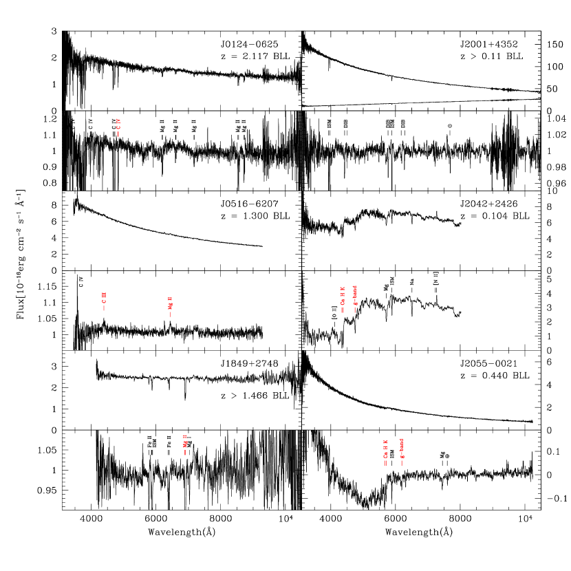
Figure 1.— Spectra of Fermi BLLs. Each object is presented twice – directly in the upper panel, and then with the best-fit power law ‘removed’ (generally by division, but for composite spectra by subtraction). This residual is plotted in the lower panel. SDSS spectra, while discussed in Table 3, are not replotted in this Figure. The six sample spectra here illustrate major trends. Similar figures for the full BLL sample are available in the electronic edition of this journal. There we mark only the two lines used to secure $z_{\rm spec}$; here other lines of interest are marked and the two qualifying lines are marked in red. $z$ limits given are the most constraining limits presented—2 digits are given for limits from non-detection of host galaxies; 3 digits, for intervening absorption systems. The marked absorption system is the best spectroscopic limit; in some cases, a stronger host galaxy limit is presented. See Table 3 for the precise spectroscopic limit.

2.4. General Trends

To illustrate the principal trends in the BLL spectra we refer the reader to Figure 1. By definition, the dominant component is a power-law. J0516$-$6207, however, shows that after removal of a power-law weak, but broad C IV, C III, and Mg II features may occasionally be seen in high S/N spectra. Here the equivalent widths ($<1$ Å) are sufficiently small to secure the identification as a BLL. However, should the continuum fade by $\sim 10\times$, this would be classified (at that epoch) as an FSRQ. Such transition objects support the idea of a Blazar continuum, rather than two distinct populations (Fossati et al., 1998; Ghisellini & Tavecchio, 2008). In S12, we reported significant broad line measurements for 5 of our BLL, including J0516-6207.

While the power-laws of most BLL are very blue, like J0516$-$6207, a few like J1849+2748, appear intrinsically flat or red, even after correcting for Galactic extinction. This may plausibly be a sign of a synchrotron component peaking near the optical, but might also indicate incomplete extinction correction, with residual reddening caused by dust not in the Schlegel et al. (1998) maps. It could also be intrinsic host extinction.

The Galactic reddening can be very severe. For J2001+4352 (upper right) we show both the highly extincted, pre-correction spectrum and the blue post-correction power law. This source is in a direction of known high $A_{V}=1.75$. Such extincted power-law spectra provide an excellent opportunity for ISM studies: The features seen after de-extinction and division by the best-fit power law (lower panel) are all interstellar in origin – Galactic H and K, Na I 5892, and a series of diffuse interstellar bands, as described in Yuan & Liu (2012).

For J0124$-$0625 (upper left) the residual absorption features are intergalactic in origin. Redward of $3900$ Å we detect a number of metal-line systems, blueward one sees the onset of strong Lyman-$\alpha$ forest absorptions. These features determine a redshift $z=2.117$ (one of the highest in our BLL sample). The lack of similar Ly$\alpha$ forest absorption in many of our other high S/N, high resolution spectra allows us to place statistical upper limits on the redshift as described in §3.3.

Finally at lower right we see two BLL with significant flux from the host. In J2042+2426, the galaxy provides about a third of the total flux and is easily visible in the raw spectrum. This is still safely a BLL, and we can measure the continuum contribution by a ‘Non-Thermal Dominance’ (see §5, here NTD=1.38). For J2055$-$0021, the host is swamped by the core synchrotron emission (NTD=47.5) and the galaxy features are visible only after subtracting the best-fit power law, as in the lower right panel. The flux increase in the blue appears due to residual few-% fluxing errors (here, likely incomplete correction for atmospheric extinction), rather than intrinsic emission. Despite the careful calibration, such residual fluxing issues persist in several spectra. However, the high-pass filtering described in §3.4 ensures that our measurements of, and bounds on, host galaxy flux are almost completely immune to such residual calibration artifacts. We find that a number of BLL show visible host galaxy components, all consistent with giant ellipticals (Urry et al., 2000). We discuss the flux distribution of these host galaxies in §3.7.

2.5. Individual Objects

A number of BLL reductions required special treatment. For example a few objects clearly required changes to the Schlegel map $A_{V}$, so that the de-extinction resulted in clean power laws. For J0007+4712, $A_{V}$ was increased from 0.3 to 0.8 and for J1941$-$6211 from 0.3 to 1.0. Conversely we decreased the $A_{V}$ of J1603$-$4904 from 7.8 to 5.0 and J2025+3343, from 6.15 to 5.0. We checked the recent recalibration of the Galactic extinction maps (Schlafly & Finkbeiner, 2011), but did not find large changes, so these extinction features affecting our BLL are probably on scales below the map resolution.

J1330+7001 was observed off of the parallactic angle—the ensuing drop in blue flux is not intrinsic to the system, and our power law is fit only redward of $5000$ Å. We thus remove the broadband residual in our power law divided spectrum in Figure 1. J1829+2729 and a nearby star were spatially unresolved in our data. The presented spectrum is a composite of starlight and quasar light, which the significant emission features all identified as $z=0$ stellar or ISM features.

In a few cases, objects previously cataloged as BLLs do not have sufficient S/N in our spectra for a definitive BLL classification. For J0801+4401, we find that undetected broad lines could have an equivalent width as large as 9.5 Å; for J0209-5229 the limit is 5.6 Å, for J1311+0035 the limit is 8.0 Å and for J1530+5736 we could have missed lines as strong as EW=5.5 Å. As higher S/N spectroscopy would likely confirm the archival BLL designations, we consider them BLLs for the purposes of this paper.

Five of the BLL described here had high significance broad line detections and have already been described in S12; we re-measure these spectra here for a uniform BLL treatment. In J0847$-$2337 and J0430$-$2507, the flux and spectral index measurements differ from the S12 values. This is because in the present analysis we first subtract the host galaxy flux, and calculate the flux and spectral index of the remaining non-thermal component. In S12, no such correction was attempted.

3. Measuring BLL Redshifts

The opportunity to advance our understanding of BLL evolution with the large, flux limited Fermi sample is important (Ajello et al., 2012b). Yet, despite the substantial telescope resources and careful analysis summarized above, many BLL did not yield direct spectroscopic redshifts, due to the extreme weakness of their emission lines (Sbarufatti et al., 2005b) and lack of clear host features. Therefore we collect here both the direct redshift measurements and quantitative constraints on the allowed redshift range for our observed BLL.

3.1. Emission Line Redshifts

We visually inspected all spectra for AGN emission line features, and host galaxy absorptions. Spectroscopic redshifts are measured by cross-correlation analysis using the rvsao package (Kurtz & Mink, 1998). We require one emission line to be present at the $>5\sigma$ level, and a second line present at the $>3\sigma$ level—significances are measured by fitting a Gaussian template in the splot tool; we allow the width and amplitude of the Gaussian to vary, but fix the center at the redshift derived by rvsao’s xcsao routine. For this study, we limited our search to typically strong emission lines known to be present in some BL Lacs: Broad emission from C IV (1549, 1551 Å), C III (1909 Å), Mg II (2796, 2799, 2804 Å), H$\gamma$ (4340 Å), H$\beta$ (4861 Å), and H$\alpha$ (6563 Å) and narrow emission from [O II] (3727, 3729 Å), [O III] (4959, 5007 Å), and [N II] (6549, 6583 Å). While other species exist in our spectra, these here listed are sufficient for definite redshift IDs. Velocities are not corrected to helio-centric or LSR frames.

In many cases, spectroscopic redshifts are further determined by a significant ($>3\sigma$) detection of a host galaxy, as will be described in §3.4. A few redshifts require further note: In J0124-0625 and J1451+5201, we identify the redshift by a Ly$\alpha$ and C IV absorption system at the onset of the Ly$\alpha$ forest. In J0434-2015, we identify a single strong feature with [O II], consistent with weak Mg II and Ca H/K absorptions. For J1728+1215, we find strong Mg II, confirmed by [O II] at the same $z$ in an archival spectrum. In J2152+1734, we identify a strong feature with Mg II confirmed by a significant [O II] detection in archival spectroscopy.

For a few objects only a single emission line was measured with high S/N. In general we use the lack of otherwise expected features to identify the species and the redshift with high confidence. Nevertheless, a few redshifts have some systematic uncertainty and are marked by a ‘:’ in Table 3. We briefly discuss these cases here. For J0007+4712, we derive a redshift from the clear onset of the Lyman-$\alpha$ forest and report only two significant figures. In J0212+2244, we determine a tentative $z$ from weak Ca H, K and g-band absorptions. For J0439-4522, we identify the one strong emission feature as C IV; intervening absorption excludes a Mg II identification, but a less likely C III identification at $z\sim 1.45$ is not conclusively ruled out. J0629$-$1959 presents broad but weak emission at the redshift of the highest $z$ metal line absorption system (1.724). We thus identify this, tentatively, as the object’s true $z$. For J0709$-$0255, we identify the strong feature at 9200 Å with [O III] by the line shape; an [O II] identification at $z\sim 0.84$ is not excluded. For J0825+0309, we find significant [O III] emission at 5007 Å (and possible, but not significant emission at 4959 Å), at a $z$ consistent with an Mg II feature identified in Stickel et al. (1993). We find weak features in J1231+2847 at the SDSS $z$, but they have low significance. For J1312$-$2156, we find a plausible Mg II feature; this single line identification is in a small allowed redshift range ($z\sim 1.6$), other identifications for this line are spectroscopically excluded. In J1754-6423, we tentatively identify emission at $\sim 6300$ Å with Mg II—higher $z$ redshifts are excluded by the lack of Ly$\alpha$ forest. In J2116+3339’s spectrum, a significant broad emission feature is identified with C IV, consistent with a weak bump in the far blue at Ly$\alpha$. Nevertheless a lower $z$ redshift is possible if the purported Ly$\alpha$ line is not real. J2208+6519 presents one strong, broad emission feature, tentatively identified as Mg II—a C IV identification at $z\sim 1.8$ is not excluded.

3.2. Intervening Absorbers

For some BLLs, the core light passes near an intervening galaxy on its way to Earth. At small radii one can encounter low excitation clouds in the galaxy’s halo, giving absorption doublets from Mg II at (2795.5, 2802.7) Å. Larger impact parameters can sample C IV at (1548.2, 1550.77) Å. In some low excitation (i.e.: Mg II) systems, we also see absorption from Fe II at (2344.2, 2374.4, 2382.7, 2586.6, 2600.1) Å. Finally, for our highest redshift BLL we Lyman-$\alpha$ absorption at 1215 Å  for the metal line systems, as well as onset of the Lyman-$\alpha$ forest.

For unsaturated absorptions, the doublet ratio for Mg II and C IV is 2:1, with the blue line dominant. In saturated absorptions, the ratio is 1:1 (Nestor et al., 2005; Michalitsianos et al., 1988).

We visually search all spectra for candidate doublets, and follow Nestor et al. (2005) in employing a quantitative test of the significance of each candidate. We used a two Gaussian template with wavelength spacing scaling with $z$, but free amplitudes, and fit the equivalent width and error of each component, using the splot tool in iraf. For the candidate to qualify as a detection we require the stronger (bluer) line to have $>5\sigma$ significance, and the second line to have $>3\sigma$ significance. In a few cases, one component of an otherwise strong doublet was affected by skylines, telluric features or cosmic rays. In these cases, another expected feature from the absorption complex (e.g.: a Fe II line) detected at $>3\sigma$ qualified the system. We further require the doublet ratio to be consistent (within errors) to a value between 2:1 and 1:1.

Our principal goal is not an absorption line study. Thus we concentrated on the longest wavelength (highest $z$) candidate system and measured sufficient lines to confirm the $z$ (i.e: two significant lines). After validation we continued to search for higher $z$ until no candidates passed the significance test. We therefore believe that we have found the highest $z$ absorption system in each of our spectra strong enough to reach the $5\sigma/3\sigma$ criteria above.

Since we see the onset of the Lyman-$\alpha$ forest in our highest redshift objects, the red end of the forest provides a strict lower limit on redshift.This can be higher than that inferred from the reddest metal line system.

We list these spectroscopic minimum $z$’s as $z_{\rm min}$, when available, in Table 3.

3.3. Redshift Upper Limits

We can use the absence of Lyman-$\alpha$ absorptions to provide statistically-based upper limits on $z$ for all BLLs without redshift. The exclusion $z_{\rm max}$ depends on the spectral range, resolution and S/N of the particular observation, but is generally $1.65<z<3.0$.

To quantify the upper bound, we need the expected density of Ly$\alpha$ forest absorbers. Penton et al. (2004) find that for rest EW $\geq 0.24$ Å, $dN/dz\sim 40$ at $z=1.6$, varying with redshift as $\log dN/dz\propto 1.85\log(1+z)$. We follow Weymann et al. (1998) for the EW scaling: $dN/dz\propto e^{-(EW_{\rm rest}-0.24)/0.267}$. As the S/N and resolution of our data vary, we generally measured a conservative uniform $3\sigma$ sensitivity for narrow Ly$\alpha$ absorptions $100$ Å from the blue end of our spectra. Typical EW limits in this range were $\sim 0.2-1.0$ Å. Given this density we solve for the $\Delta z$ range giving a Poisson probability of $0.32$ (ie: $1\sigma$) for detecting no absorbers, obtaining:

$$\Delta z=0.167\cdot e^{(EW_{\rm rest}-0.24)/0.267)}\cdot\left(\frac{\lambda_{\rm min}}{1215}\right)^{-1.85}$$ (1)

where $\lambda_{\rm min}$ is the effective blue end of the spectrum (generally 3150 – 4200 Å), and EW is the measured equivalent width limit. Thus, we infer a maximum source redshift $z_{\rm max}=(\lambda_{\rm min}/1215)-1+\Delta z$. In some cases, the S/N is too low at the blue end of the spectrum. We then measure EW limits closer to the sensitivity peak of the spectrum. Of course, with a larger $\lambda_{\rm min}$ for the effective spectrum end Equation 1 gives less constraining upper limits.

If the actual blazar redshift $z$ is very close to $z_{\rm max}$ as estimated above, then its UV radiation may photo-ionize Ly$\alpha$ clouds along the line of sight, postponing the onset of the forest and artificially lowering $z_{max}$. In practice, the effect is usually small ($\Delta z_{max}\sim 0.01-0.02$) except for large $z_{max}$ when our bound is generally not of interest. We follow Bajtlik et al. (1988) to estimate this ‘proximity effect’ correction, by computing

$$\omega(z_{\rm Ly\alpha})={{f_{\nu}}\over{4\pi J_{\nu}}}{{(1+z_{\rm Ly\alpha})^{5}}\over{(1+z)}}\left[{{(1+z)^{1/2}-1}\over{(1+z)^{1/2}-(1+z_{\rm Ly\alpha})^{1/2}}}\right]^{2}$$ (2)

where $f_{\nu}$ is the blazar flux at the absorption Lyman limit (at $z_{\rm Ly\alpha}$) and $J_{\nu}=10^{-21.5}{\rm erg\,cm^{-2}\,s^{-1}\,Hz^{-1}\,sr^{-1}}$ is the cosmic ionizing flux, conservatively estimated for our redshift range. We compute $f_{\nu}$ from the power law fit in Table 3, and increase the blazar redshift $z$ until $\omega(z_{\rm Ly\alpha})<1$. We thus adopt these revised $z_{max}=z$ and quote these corrected upper limits in Table 3.

3.4. Host Galaxy Fitting

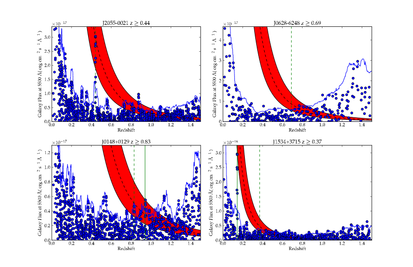
Figure 2.— Best fit host galaxy fluxes as a function of trial $z_{i}$ (blue dots). Our estimate of the $2\sigma$ local systematic flux error is shown by the blue line (see text). The red bands give the $1\sigma$ range about the expected host flux for $M_{R}=-22.5\pm 0.5$. Vertical green dashed lines give our $z_{\rm min}(-22.5)$ limit on the redshift. For comparison, solid green lines give the spectroscopic redshifts, when measured. For J2055$-$0021 and J0148+0129 these are consistent; the former has a high significance host detection (Figure 1), while for the latter the higher $z$ redshift is from emission lines. J1534+3715 is one of 9 objects with limits inconsistent with spectroscopic redshifts. Here, the host galaxy is sub-luminous ($M_{R}=-21.87\pm 0.16$) and thus (just) missed by this technique (Prob = 0.15).

It has been claimed that BL Lac objects are hosted by giant elliptical galaxies with bright absolute magnitude – $M_{R}=-22.9\pm 0.5$ in our cosmology (Urry et al., 2000; Sbarufatti et al., 2005b).

If we adopt the common assumption that these are standard candles, we can estimate the redshift of the BLL by detecting such galaxies. In imaging studies, one looks in the wings of the BLL for the host galaxy flux, and compares that to the standard candle flux at various redshifts (Sbarufatti et al., 2005a; Meisner & Romani, 2010). In spectroscopic studies, one typically looks for individual absorption features (i.e.: H, K, g-band). One can also use the lack of such lines as evidence that the BLL is at higher redshift (Sbarufatti et al., 2005b; Shaw et al., 2009).

With high S/N spectra, however, one can obtain more stringent limits by using the entire elliptical template rather than just one (or a few) lines. Plotkin et al. (2010) developed a technique of fitting for host galaxies in SDSS BLL spectra. We expand here on that method for our more heterogeneous spectra.

Our spectra come from a variety of spectrographs in disparate observing conditions and we find low frequency systematic fluctuations in many of the fits. These are likely caused by imperfect spectrophotometric fluxing and second order contamination as discussed in §2.3. These effects can dominate over real galaxy features. Using SciPy’s Signal Processing routines, we construct a bandpass Kaiser window from 220 Å  to $1.5\times$ the Nyquist frequency. We apply that window as an effective high pass filter both to our spectra and to the templates, to mitigate this low-frequency noise before fitting (Kaiser & Schafer, 1980).

We test possible redshifts $z_{i}$ on a grid scaled to the spectrograph resolution with constant spacing in $\log z$. This grid is thus $z_{i}=(\frac{2\Delta\lambda}{\lambda_{0}}+1)^{i}-1$, where $\Delta\lambda$ is the pixel scale of the spectrograph. For each trial $z_{i}$ we fit the power law $F_{\nu}\propto\nu^{\alpha}$ index and flux and the amplitude of a redshifted elliptical template. This host template is generated from the PEGASE model (Fioc & Rocca-Volmerange, 1997) tables and evolved to low $z$ from $z=2$, as in O’Dowd & Urry (2005). For uniformity, we here use the same template for all $z_{i}$, and do not perform any evolution corrections.

Our fit minimizes $\chi^{2}$ with three free variables at each trial $z_{i}$. We employ the scipy.optimize.leastsq routine based on a Levenberg-Marquardt fitter.

To model host slit losses, we assume an $r=10$ kpc de Vaucouleurs profile with Sersic index 1/4 (O’Dowd & Urry, 2005) and account for the individual observations’ slit width and seeing profile (measured from the core full width at half maximum, FWHM). Since we have employed optimal extractions of the BLL spectra, our effective aperture along the slit varies, but we estimate a typical width of $\approx 2\times$ the spatial FHWM achieved during our spectral integration. Accordingly we estimate host slit losses through a rectangular aperture of the slit width $\times$ twice the spectrum FWHM. Inferred host fluxes are corrected for these slit losses.

Results of sample fits are shown as the blue dots in Figure 2 where the fit amplitude of the host galaxy template is plotted against trial redshift.

3.5. Power Law Fit

We report the power law fluxes and spectral indices of the best fit to the de-extincted spectrum in Table 3. The flux is given in units of Log $10^{-28}$erg cm^-2s^-1Hz^-1 as observed at $10^{14.7}$ Hz ($\sim 5980$ Å), the center of our typical spectral range. The index $\alpha$ is measured $F_{\nu}\propto\nu^{\alpha}$. These values may be combined with multi-wavelength data to study the continuum SED of the blazars in our sample. Since the statistical errors on the fit are, in general, unphysically small, we follow S12 in estimating errors on the spectral index by independently fitting the red and blue halves of the spectrum. Note that large errors bars generally indicate a relatively poor fit to a simple power law rather than large statistical errors. The statistical errors on the $F_{\nu}$ amplitude are also small; we convolve these with our estimated $30\%$ overall fluxing uncertainty (Healey et al., 2008), which dominates in nearly all cases.

Figure 3.— Histogram of maximum flux ratios. For each object where we have collected multiple spectra, we compute the flux ratio between the power law components of the brightest and faintest observed epoch. These are plotted as a log-log histogram. The dashed line is the best-fit power law with index $\alpha=1.29$. The inset histogram shows the distribution of time between observations – typically $\sim$ 1 year

For objects with high significance ($>3\sigma$) detections of galaxies, as described in §3.7, we report the best fit power law from the simultaneous power-law/host fit in §3.4.

When we have observed objects at multiple epochs, we also fit a power law to the other, non-primary spectra. These fluxes vary substantially, some by more than $10\times$. In Figure 3, we show the distribution of $f_{\rm max}/f_{\rm min}$ flux ratios. This is well-described by an $\alpha=1.29$ power law. Epochs from our fiducial spectra are listed in Table 3.

3.6. Testing the Standard Candle Assumption

BLL with a redshift and a secure ($>3\sigma$) host detection can be used to test the uniformity of the host luminosities. There are 59 such BLL in our sample. We derive synthetic $R$-band magnitudes by applying a Kron-Cousins R filter to our spectra (Meisner & Romani, 2010). The results are shown as a histogram in Figure 4. We find $<M_{R}>=-22.5$, down $\sim 0.4$ magnitudes from $M_{R}=-22.9$ found in Sbarufatti et al. (2005b). We find a similar spread in luminosity ($\sim\pm 0.5$ magnitudes). When we separate the host measurements for lower-peak sources (LBL+IBL) we find that they have a median luminosity $\sim 0.3$ magnitudes fainter than that of our HBL. Unfortunately, we do not have sufficient LBL+IBL hosts to test for such differences at high significance. Past studies differ: Urry et al. (2000) found no significant offset in the host magnitudes of HBL and LBL, but Sbarufatti et al. (2005b) noted that higher peak HBL tend to have more luminous hosts.

Two of the high significance host galaxies have imaging magnitudes reported in Sbarufatti et al. (2005b). For J1442+1200, we measure $M_{R}=-22.99\pm 0.14$; Sbarufatti et al. (2005b) reported $M_{R}=-22.77$. For J1428+4240, we measure $M_{R}=-22.78\pm 0.13$; Sbarufatti et al. (2005b) find $M_{R}=-22.75$. These are consistent within measurement errors, a good check of our slit-loss corrections and magnitude estimates.

Overall, the LAT BLL sample thus represents a fainter host population of than those studied in previous work. Conceivably a higher (LBL+IBL)/HBL ratio in our sample causes part of the difference (although we remain HBL dominated). However, we suspect that our rather exhaustive $8$-m class campaign, skipping most objects with redshifts already in the literature, selects for fainter host galaxies than in the past. Thus we may be probing fainter on the true host luminosity distribution; the BLL for which we were not able to provide host detections may then be similarly under-luminous compared to previous studies. A true evaluation of the intrinsic host luminosity distribution, as well as any dependence on subclass type, will require a careful assessment of the parent population ($\gamma$-ray) and host detection selection biases.

In the rest of this section, we conservatively adopt our $M_{R}=-22.5\pm 0.5$ estimate. We do also report (Table 3) more aggressive redshift limits based on the common assumption $M_{R}=-22.9\pm 0.5$, for more direct comparison to previous work, but we recommend adoption of the less stringent $M_{R}=-22.5\pm 0.5$ redshift constraints.

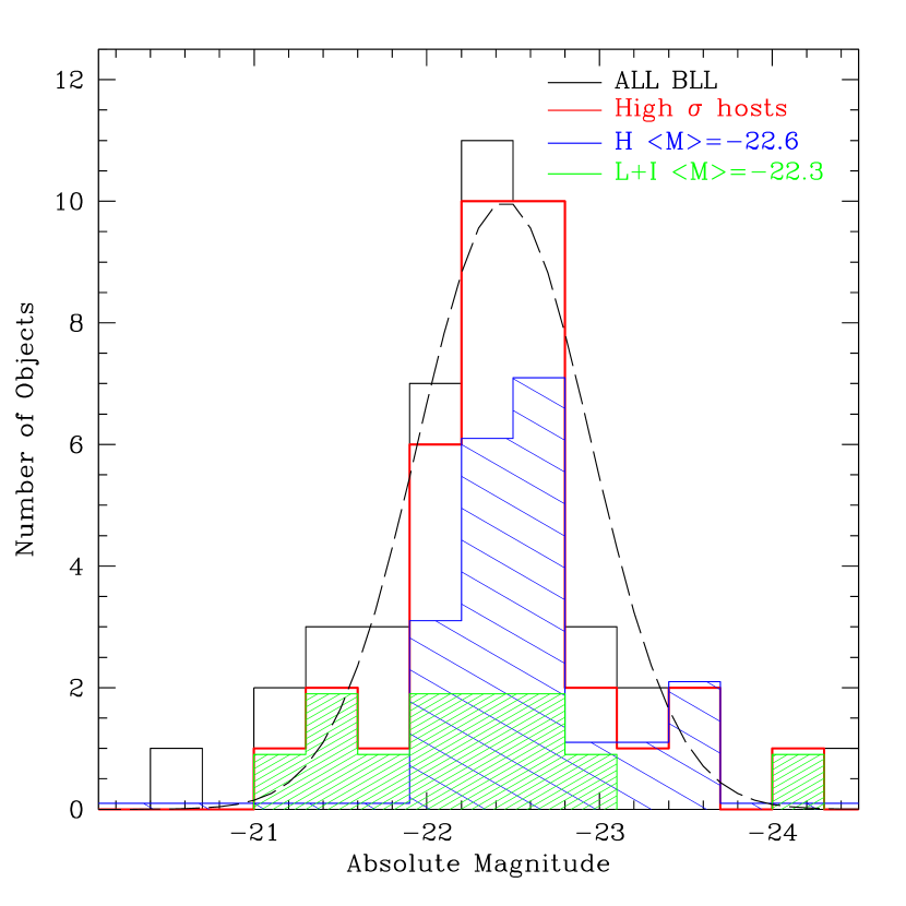
Figure 4.— Measured BLL host absolute magnitudes ($R$ equivalent at $z=0$). Black histogram: all BLL hosts with spectroscopic redshift. A weighted $\chi^{2}$ fit gives $M_{R}=-22.5\pm 0.5$, our best estimate for the luminosity of BLL host galaxies. Red: hosts with high significance ($>3\sigma$) detections. Green and Blue sub-histograms show high significance LBL+IBL and HBL hosts, respectively.

3.7. Lower Limits from Non-detections of Host Galaxy

We use the results of the fitting in §3.4 and the calibration in §3.6 to constrain the redshift of the host. At each trial redshift, our fitter reports a flux ($f\pm\sigma f$) for the host galaxy. This is to be compared with the model flux from the redshifted standard candle elliptical template ($f_{M}\pm\Delta f_{M}$).

While we have greatly decreased the effect of the low frequency noise in our spectral fits using the high-pass filter, we still find that the statistical errors on the fit host galaxy fluxes are unrealistically small; these flux estimates remain dominated by systematic effects. We therefore construct an error estimate $\Delta f$ for each $z_{i}$ by measuring the dispersion of flux estimates for nearby redshift bins. This is computed from a sample of the 30 nearest $f(z)$, skipping 5 bins on each side of our test $z_{i}$ to minimize high pass correlation. After $\sigma$-clipping, the fit flux distributions are well behaved and we use these to compute a 2-$\sigma$ upper limit (scaled from the rms) at each $z_{i}$. Vectors of these upper limits are shown by the jagged blue lines in Figure 2. These have captured the local effective noise quite well and so we adopt these vectors as effective $2\sigma$ confidence limits.

Fit fluxes well above these $2\sigma$ limits denote likely host detections. Indeed, we found that this automatic processing was quite effective at flagging candidate $z_{i}$ for host detection. Here, however, we focus on how well a fit flux $f$ with local effective error $\Delta f$ can be used to exclude a host of the expected magnitude $f_{M}$ at the test redshift $z$. Thus we compute a probability that the fit flux $f$ and error $\Delta f$ are consistent with the expected model flux $f_{M}$ and its uncertainty at the given $z$ as

$$Prob(z;f,\Delta f)=C\int_{f_{M}}^{\infty}G(f^{\prime}_{M},\Delta f^{\prime}_{M})\cdot G(f,\Delta f)df^{\prime}_{M}$$ (3)

where $G(x,\sigma_{x})$ is a Gaussian of width $\sigma_{x}$ centered at $x$. The normalization $C$ is chosen such that $Prob=1$ for $f_{M}=0$ (i.e.: any $f$ is acceptable for a model of zero flux). This is a conservative choice as it does not exclude over-luminous hosts. For example, when we assume a model $M_{R}=-22.5\pm 0.5$ this probability also finds any $f$ consistent with $M_{R}=-22.9\pm 0.5$ to be acceptable. When the fitter returns an unphysical negative $f$, we evaluate the probability for $f=0$ and the local $\Delta f$.

This probability becomes substantial for $z$ near a good candidate redshift. It also grows as the sensitivity of our host search drops at large $z$. We thus calculate a minimum redshift ($z_{min(-22.5)}$) as the lowest redshift for which $Prob\geq 0.17$ (i.e.: $1\sigma$). We list these values in Table 3. For comparison, we also give $z_{min(-22.9)}$ calculated in the same fashion, assuming a model $M_{R}=-22.9\pm 0.5$. Comparison between the spectroscopic detections and $z_{\rm min}$ suggest that the $M_{R}=-22.5$ value is most consistent with observed detections, and lower bounds (as expected from §3.6). We recommend use of these conservative lower limits. Note also that the vector $Prob(z)$, once normalized with an appropriate prior and truncated at $z_{\rm max}$, can be used as a PDF for the BLL redshift.

3.8. Redshift Distribution

As seen in Figure 5, archival redshift measurements for BLL are dominated by low values ($\tilde{z}=0.23$). Our new spectroscopic redshifts have extended the population to higher $z$, with some objects’ redshifts at $z\gg 1$. Still, the objects with redshifts remain dominated by low $z$. In the new spectroscopic redshifts we find $\tilde{z}=0.33$. We believe there is a significant bias to low redshift in both of these samples, as the weak low EW emission or absorption features of our typical BLLs with known redshift are easier to detect at low $z$.

In Figure 5 we also show two sets of redshift lower limits. For every object in our sample, we can derive a host-detection limit ($\tilde{z}=0.41$). These lower limits on redshift are still biased low: as evident from Figure 2 we are most sensitive to galaxies at low $z$. Nevertheless, they suggest that these objects are not consistent with the spectroscopic redshifts (the K-S test gives probability $<10^{-11}$ of consistency with archival redshifts). The absorption line limits we have for some objects (described in §3.2) give further evidence for a population of BLLs at high redshift ($z>1$). Together, these results strongly imply that previous BLL studies suffered important biases due to shallow samples with large redshift incompleteness preventing detection of bright, but high $z$ BLL.

The inset shows the spectroscopic redshifts and the redshifts limits for high-peaked (HBL) and lower-peaked (LBL+IBL) sources classified in 2LAC. We see that the lower-peaked detections extend to higher z, as might be expected if these sources are more luminous and have a less dominant synchrotron continuum. However, the open histograms of limits remind us that both sub-classes still suffer substantial redshift incompleteness, and the missing redshifts for both sub-classes extend substantially higher than those in hand. A re-appraisal of the BLL population, properly including the new redshifts, $z$ constraints and remaining selection biases is needed to test whether either subclass is still consistent with negative cosmological evolution.

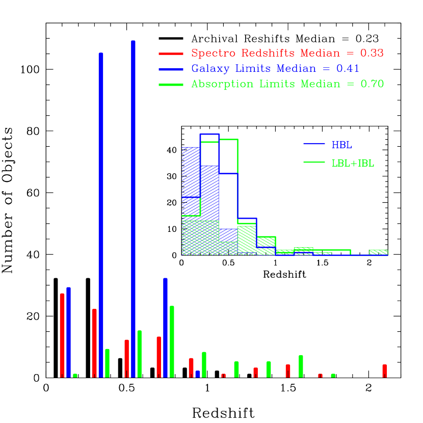
Figure 5.— BLL redshift and redshift lower limit distributions. Within each $\delta z=0.2$ bin, we show (left to right) the Archival $z$, our new spectroscopic $z$, lower limit $z$’s from host fitting and lower limit $z$’s from intervening absorption line systems. The limits show that the spectroscopic redshift samples, particularly the archival sample, are selection biased to low $z$. The subframe shows the redshifts (filled histograms) and lower limits (open histograms) for the LBL+IBL (green) and HBL (blue). Again, both limit histograms extend to higher $z$. The LBL+IBL sample extends somewhat further than the HBL.

4. Black Holes and Host Galaxies

The masses of the central black holes provide important insight into the cosmic evolution of various AGN classes. These are most easily estimated by the virial technique (cf., Shen et al., 2011). In S12, we adopted this method to give mass estimates for the Fermi FSRQs. For BLL, the lack of high S/N broad line measurements precludes such estimates. However, we have measured a number of host magnitudes in §3.4; since these are ellipticals, this is all ‘bulge,’ and we can apply an $M-L$ relation to estimate the hole mass. We follow Gültekin et al. (2009):

$$\log\left(\frac{M}{M_{\odot}}\right)=(8.95\pm 0.11)+(1.11\pm 0.18)\log\left(\frac{L_{V}}{10^{11}L_{\odot,V}}\right)$$ (4)

where $M$ is the black hole mass, and $L_{V}$ is the luminosity in a $V$ filter [$\log(L_{V}/L_{\odot,V})=0.4(4.83-M^{0}_{V,{\rm bulge}})$]. To convert our fit template spectrum amplitudes to consistent V magnitudes, we integrate our template spectrum over the Hubble F555W filter (Lauer et al., 2005) as in §3.6.

The masses from Equation 4 are plotted as circles in Figure 6. When the sub-class is known (HBL or LBL+IBL) we fill these in with blue or green, respectively. For comparison, we show the $1\sigma$ spread of virial-estimate BH masses from optically selected SDSS quasars from Shen et al. (2011) (gray band) and masses of the Fermi FSRQs in S12 (red points). Of course, if BLL hosts really are standard candle ellipticals, then the $M_{bulge}-M_{\bullet}$ relation implies constant black hole masses. The masses corresponding to the standard $M_{R}=-22.9$ and our revised $-22.5$ are shown by dashed lines.

Interestingly, our BLL $M_{\bullet}$ estimates increase with $z$ much as the optical QSO or FSRQ. Of course, we only plot high significance host detections here, and low luminosity hosts at high $z$ are increasingly difficult to detect (unless the core luminosity decreases). Accordingly, as for the QSO, we suspect that the bulk of this trend is due to selection effects. In the case of the FSRQ, S12 argued that the offset to smaller black hole mass was at least partly due to a preferentially polar view of an equatorially flattened broad line region, with the projection decreasing the observed kinematic line width and the average virial mass estimate. Like $\gamma$-ray selected FSRQ, BLL are Doppler-boosted along our line of sight (Urry & Padovani, 1995). However since the host flux is nearly isotropic, we expect little alignment bias in our $M_{\bullet}$ estimates. Thus, it is unclear whether the BLL offset to larger black hole masses is real or selection dominated.

In a study of BLL hosts detected in the SDSS León-Tavares et al. (2011) found no significant difference between the masses of the central black holes of HBL and LBL. In figure 6 the HBL masses are however biased upwards with respect to the lower-peak BLL black hole masses. This is of course just a restatement of the offset in host luminosity seen in Figure 4. Unfortunately, we cannot claim that this is a physical difference as the trend is precisely what would expect from selection bias if HBL have brighter non-thermal cores.

Ideally we could use these black hole masses to explore the relationship between the BLLs and the general QSO population. Large black hole masses, if not induced solely by selection bias would imply a late stage of AGN evolution. The black hole mass is often compared to the source luminosity to characterize the state of the accretion in Eddington units. However, with the exception of the few BLL for which we see broad lines (which seldom have a significantly host detection), the observed flux is so dominated by beamed jet emission that quoting the accretion luminosity in Eddington units is not feasible.

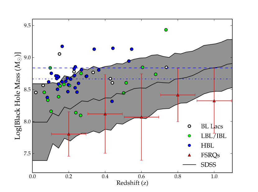
Figure 6.— BLL black hole masses plotted as a function of redshift (circles; blue fill HBL, green fill LBL+IBL). The gray band shows the $1\sigma$ spread of the optically selected SDSS black holes (Shen et al., 2011). Red error bars give the $1\sigma$ spread Fermi FSRQ black hole masses (S12). The estimated BLL black hole masses are higher than for the two other AGN types. The upper (lower) blue lines show the black hole mass expected for the standard candle bulge at $M_{R}=-22.9(-22.5)$.

5. Non-thermal Dominance

In S12, we introduced the non-thermal dominance (NTD) as a quantitative measure of how much the optical is contaminated by non-thermal synchrotron emission. We here extend that analysis to BLLs.

For most BLL, the dominant ‘thermal’ contribution is the host galaxy, not the big blue bump. We therefore set $NTD\equiv F_{\rm core}/F_{\rm host}$ where both fluxes are measured at 5100 Å – the same wavelength as the H$\beta$ continuum measurements for FSRQs. The wavelength choice is important for BLL NTD measurements, since the host galaxy is much redder than the continuum-dominated core; an NTD measurement just above (redward of) the $4000$ Å break would typically give values $\gtrsim 4\times$ larger. Measurements below the break would, of course, diverge even more.

As noted BLL are highly variable, so that their NTD changes over time. Our BLL can vary by over an order of magnitude in the optical (S12, Fig. 3). In this study, our primary spectra for variable objects were generally drawn from the epochs giving the highest signal to noise on weak emission or absorption features. As this favors low core fluxes, our primary epoch biases the results towards low NTD.

In Figure 7, we plot the NTD against $\gamma$-ray spectral index. The values for BLL with measured galaxy flux are plotted, along with lower limits for BLL with redshift, but no significant host detection. The histogram at right shows the spectral index distribution of BLL with no redshift detection (and unknown NTD). We expect these BLL to have higher NTD on average, as the larger core flux makes redshift determinations more challenging. When known, we indicate whether the BLL are high-peaked sources (blue) or lower-peaked (green). The FSRQs from S12 are plotted as red triangles.

The most striking trend in this figure is the vertical color separation. This is the well-known result that $\gamma$-ray spectral index hardens from FSRQ through LBLs to HBLs (Ackermann et al., 2011). We also see the defining characteristic of the BLL, increased continuum dominance with respect to the FSRQ. However, the NTD trend does not appear to continue through the BLL: harder spectrum BLL do not in general show increased NTD. Indeed the highest NTD seem to be associated with LBL/IBL measurements and lower bounds. A plausible interpretation is that the LBL/IBL are more luminous and hence visible to higher $z$, where we are less likely to detect a host galaxy.

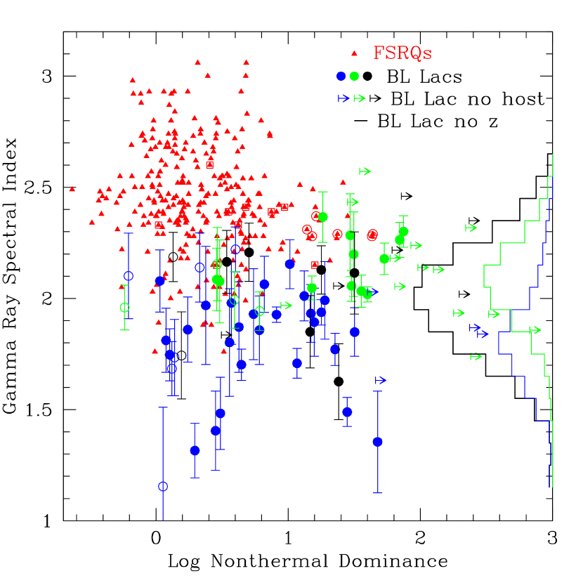
Figure 7.— The NTD plotted against $\gamma$-ray spectral index. The BLL are plotted as dots; solid if $L_{\gamma}>10^{44}$; empty otherwise. Broad line objects from S12 (typically FSRQs) are plotted as red triangles – circles surround those in a BLL state at the primary spectrum epoch; squares, those known to be BLL at a different epoch. BLL with known $z$, but no thermal (host galaxy or broad emission line) detection are plotted as lower limits. BLL without known $z$ are shown by the histogram at right. Blue symbols indicate HBL, green LBL+IBL. Except for the NTD increase for the BLL population relative to the FSRQ, no clear trend with spectral index is seen.

6. Conclusions

We have dramatically increased the redshift completeness of this largest ever $\gamma$-ray selected BLL sample; $\sim 44\%$ of these BLL now have spectroscopic redshifts, and $\sim 95\%$ have at least a strong lower bound on the redshift. These $z$ constraints show that the subset with actual spectroscopic redshifts is strongly biased to low $z$. Although we find that the measured redshifts for low-peaked BLL (LBL+IBL) do extend higher than those for the HBL with the highest synchrotron peak, our set of lower limits for both subclasses extend to yet higher $z$ than the spectroscopically solved objects. Thus the actual redshifts for all BLL are biased low compared to a flux-limited parent population of $\gamma$-ray BLL. This must be taken into account in any study of BLL evolution over cosmic time (Ajello et al, in prep).

Many of our redshift limits rely on the common assumption that BLL hosts are standard candles. Our effort to re-calibrate the standard luminosity for the Fermi BLL has resulted in fainter absolute magnitudes and, hence, more conservative minimum $z$. This implies that the standard candle assumption deserves further study, which could be best prosecuted by obtaining more high spatial resolution images of BLL with known redshifts. Our study provides a large increase in the spectroscopic redshifts, a useful precursor to such work. We find limited evidence that HBL have more luminous hosts than LBL/IBL. Whether this is intrinsic or a selection effect in the presence of a brighter, harder continuum is not yet clear.

Of course true spectroscopic redshifts are always preferable for uniform population studies. However, we suspect that much higher completeness will be difficult to attain, and will likely require novel observational techniques, as significantly more time on $8$ m class telescopes is both expensive and likely to provide only marginally better results. In the interim, the best hope for progress lies with careful correction for selection effects in the present sample. Because of the tight correlation of synchrotron peak frequency with LAT-measured spectral index and because of the $\gamma$-ray index dependence of the LAT sensitivity, study of the relative population and evolution of different BLL subclasses will require correction for $\gamma$-ray selection effects as well as possible biases in the redshift determinations themselves. While we do not attempt such study here, our improved completeness will help in understanding these selection effects.

We find that BLL black hole mass estimates (at a given redshift) are larger than those for optically selected quasars or Fermi FSRQs. Associated with the apparent host luminosity differences, the present detections suggests that HBL host the largest mass black holes. We cannot at present tell whether these trends are a true difference in the black hole populations or luminosity-driven selection effects.

BLLs are, by definition, non-thermally dominated (NTD $>1$). We find the BLL population to have significant higher NTD than the Fermi FSRQs. This claim is conservative, as the objects without redshift are likely to be at even higher NTD. Since BLL have a range of $\gamma$-ray spectral index harder than those of FSRQ, it is perhaps surprising that this trend does not hold within the BLL class: NTD is not, on average, higher for the hardest-spectrum BLL. It seems likely that, in this respect at least, BLL are a distinct population from FSRQ, and not just the hardest spectrum objects on a continuum. In this case we might expect NTD to be controlled by the precise accident of the jet Doppler boosting. This accords well with the idea that NTD can vary for an individual source as the jet angle or effective Doppler factor vary, with relatively little change in the GeV spectrum. Multi-epoch, multiwavelength studies of the brighter BLL with a range of $\gamma$-ray hardness are needed to test these ideas.

Table 3BLL Spectral Properties

2FGL	RA	Dec	Name        $\log F_{\nu,10^{14.7}}$          $\alpha$			MR	$z$	ID	$z_{min}$	$z_{min}$	$z_{min}$	$z_{max}$	Type	SED	Tel.	MJD
			$10^{-28}$erg cm-2s-1Hz-1							(-22.5)	(-22.9)
J0000.9$-$0748	0.325017	$-$7.774111	J0001$-$0746	1.55$\pm$0.11	$-$1.399$\pm$0.003	…	…	.	…	0.33	0.50	1.84	BLL	IBL	P200	55064
J0007.8+4713	1.999862	47.202135	J0007+4712	1.33$\pm$0.14	$-$1.431$\pm$0.430	…	2.1:	S	1.659	0.26	0.36	2.69	BLL	LBL	P200	55743
J0009.0+0632	2.267006	6.472664	J0009+0628	1.38$\pm$0.11	$-$1.410$\pm$0.007	…	…	.	…	0.58	0.76	1.65	BLL	LBL	WMKO	55040
J0009.1+5030	2.344750	50.508005	J0009+5030	1.51$\pm$0.11	$-$0.776$\pm$0.010	…	…	.	…	0.79	0.79	1.64	BLL	…	WMKO	55475
J0012.9$-$3954	3.249804	$-$39.907184	J0012$-$3954	1.01$\pm$0.11	$-$1.248$\pm$0.032	…	…	.	…	0.52	0.64	2.52	BLL	…	VLT	54362
J0013.8+1907	3.485099	19.178246	J0013+1910	0.61$\pm$0.11	$-$2.250$\pm$0.076	…	0.477	B	…	0.41	0.54	2.17	BLL	…	WMKO	54470
J0018.5+2945	4.615626	29.791743	J0018+2947	1.13$\pm$0.11	$-$0.701$\pm$0.181	…	…	.	…	0.89	0.94	1.71	BLL	HBL	WMKO	55547
J0018.8$-$8154	4.841042	$-$81.880833	J0019$-$8152	1.73$\pm$0.12	$-$0.975$\pm$0.045	…	…	.	…	0.24	0.34	2.32	BLL	HBL	NTT	55778
J0021.6$-$2551	5.385517	$-$25.846999	J0021$-$2550	1.63$\pm$0.11	$-$0.689$\pm$0.005	…	…	.	0.564	0.57	0.58	1.63	BLL	IBL	WMKO	55476
J0022.2$-$1853	5.538158	$-$18.892486	J0022$-$1853	1.94$\pm$0.11	$-$1.061$\pm$0.069	…	…	.	0.774	0.13	0.15	1.64	BLL	HBL	WMKO	55476
J0022.5+0607	5.635264	6.134573	J0022+0608	1.86$\pm$0.11	$-$1.560$\pm$0.009	…	…	.	…	0.29	0.42	1.63	BLL	LBL	WMKO	55060
J0029.2$-$7043	7.170792	$-$70.754694	J0028$-$7045	1.38$\pm$0.11	$-$1.139$\pm$0.011	…	…	.	0.966	0.54	0.58	1.95	BLL	…	VLT	55056
J0033.5$-$1921	8.393060	$-$19.359393	J0033$-$1921	1.94$\pm$0.12	$-$0.852$\pm$0.053	…	…	.	…	0.29	0.37	1.77	BLL	HBL	P200	55567
J0035.2+1515	8.810913	15.250758	J0035+1515	1.93$\pm$0.11	$-$0.895$\pm$0.003	…	…	.	…	0.48	0.48	1.65	BLL	HBL	WMKO	55357
J0037.8+1238	9.461902	12.638514	J0037+1238	2.00$\pm$0.11	$-$1.163$\pm$0.010	$-$22.4$\pm$0.1	0.089	G	…	0.09	0.09	1.76	BLL	HBL	WMKO	55357

Note. — Table 3 is published in its entirety in the electronic edition of this journal; A portion is shown here to show its form and content.

References

- Ackermann et al. (2011) Ackermann, M., et al. 2011, ApJ, 743, 171
- Ajello et al. (2012a) Ajello, M., et al. 2012a, ApJ, 751, 108
- Ajello et al. (2012b) —. 2012b, ApJ, 751, 108
- Appenzeller et al. (1998) Appenzeller, I., et al. 1998, The Messenger, 94, 1
- Atwood et al. (2009) Atwood, W. B., et al. 2009, ApJ, 697, 1071
- Bajtlik et al. (1988) Bajtlik, S., Duncan, R. C., & Ostriker, J. P. 1988, ApJ, 327, 570
- Beckmann et al. (2003) Beckmann, V., Engels, D., Bade, N., & Wucknitz, O. 2003, A&A, 401, 927
- Bohlin (2007) Bohlin, R. C. 2007, in Astronomical Society of the Pacific Conference Series, Vol. 364, The Future of Photometric, Spectrophotometric and Polarimetric Standardization, ed. C. Sterken, 315–+
- Buzzoni et al. (1984) Buzzoni, B., et al. 1984, The Messenger, 38, 9
- Dekker et al. (1986) Dekker, H., Delabre, B., & Dodorico, S. 1986, in Presented at the Society of Photo-Optical Instrumentation Engineers (SPIE) Conference, Vol. 627, Society of Photo-Optical Instrumentation Engineers (SPIE) Conference Series, ed. D. L. Crawford, 339–348
- Fioc & Rocca-Volmerange (1997) Fioc, M., & Rocca-Volmerange, B. 1997, A&A, 326, 950
- Fossati et al. (1998) Fossati, G., Maraschi, L., Celotti, A., Comastri, A., & Ghisellini, G. 1998, MNRAS, 299, 433
- Ghisellini & Tavecchio (2008) Ghisellini, G., & Tavecchio, F. 2008, MNRAS, 387, 1669
- Giommi et al. (2012) Giommi, P., Padovani, P., Polenta, G., Turriziani, S., D’Elia, V., & Piranomonte, S. 2012, MNRAS, 420, 2899
- Gültekin et al. (2009) Gültekin, K., et al. 2009, ApJ, 698, 198
- Healey et al. (2008) Healey, S. E., et al. 2008, ApJS, 175, 97
- Kaiser & Schafer (1980) Kaiser, J., & Schafer, R. 1980, Acoustics, Speech and Signal Processing, IEEE Transactions on, 28, 105
- Krisciunas et al. (1987) Krisciunas, K., et al. 1987, PASP, 99, 887
- Kurtz & Mink (1998) Kurtz, M. J., & Mink, D. J. 1998, PASP, 110, 934
- Lauer et al. (2005) Lauer, T. R., et al. 2005, AJ, 129, 2138
- León-Tavares et al. (2011) León-Tavares, J., Valtaoja, E., Chavushyan, V. H., Tornikoski, M., Añorve, C., Nieppola, E., & Lähteenmäki, A. 2011, MNRAS, 411, 1127
- Marcha et al. (1996) Marcha, M. J. M., Browne, I. W. A., Impey, C. D., & Smith, P. S. 1996, MNRAS, 281, 425
- Meisner & Romani (2010) Meisner, A. M., & Romani, R. W. 2010, ApJ, 712, 14
- Michalitsianos et al. (1988) Michalitsianos, A. G., Kafatos, M., Fahey, R. P., Viotti, R., Cassatella, A., & Altamore, A. 1988, ApJ, 331, 477
- Nestor et al. (2005) Nestor, D. B., Turnshek, D. A., & Rao, S. M. 2005, ApJ, 628, 637
- Nolan et al. (2012) Nolan, P. L., et al. 2012, ApJS, 199, 31
- O’Dowd & Urry (2005) O’Dowd, M., & Urry, C. M. 2005, ApJ, 627, 97
- Oke (1990) Oke, J. B. 1990, AJ, 99, 1621
- Penton et al. (2004) Penton, S. V., Stocke, J. T., & Shull, J. M. 2004, ApJS, 152, 29
- Plotkin et al. (2010) Plotkin, R. M., et al. 2010, AJ, 139, 390
- Rector et al. (2000) Rector, T. A., Stocke, J. T., Perlman, E. S., Morris, S. L., & Gioia, I. M. 2000, AJ, 120, 1626
- Sbarufatti et al. (2005a) Sbarufatti, B., Treves, A., & Falomo, R. 2005a, ApJ, 635, 173
- Sbarufatti et al. (2005b) Sbarufatti, B., Treves, A., Falomo, R., Heidt, J., Kotilainen, J., & Scarpa, R. 2005b, AJ, 129, 559
- Schlafly & Finkbeiner (2011) Schlafly, E. F., & Finkbeiner, D. P. 2011, ApJ, 737, 103
- Schlegel et al. (1998) Schlegel, D. J., Finkbeiner, D. P., & Davis, M. 1998, ApJ, 500, 525
- Shaw et al. (2009) Shaw, M. S., Romani, R. W., Healey, S. E., Cotter, G., Michelson, P. F., & Readhead, A. C. S. 2009, ApJ, 704, 477
- Shaw et al. (2012) Shaw, M. S., et al. 2012, ApJ, 748, 49
- Shen et al. (2011) Shen, Y., et al. 2011, ApJS, 194, 45
- Stickel et al. (1993) Stickel, M., Fried, J. W., & Kuehr, H. 1993, A&AS, 98, 393
- Szokoly et al. (2004) Szokoly, G. P., et al. 2004, ApJS, 155, 271
- Tody (1986) Tody, D. 1986, in Society of Photo-Optical Instrumentation Engineers (SPIE) Conference Series, Vol. 627, Society of Photo-Optical Instrumentation Engineers (SPIE) Conference Series, ed. D. L. Crawford, 733–+
- Urry & Padovani (1995) Urry, C. M., & Padovani, P. 1995, PASP, 107, 803
- Urry et al. (2000) Urry, C. M., Scarpa, R., O’Dowd, M., Falomo, R., Pesce, J. E., & Treves, A. 2000, ApJ, 532, 816
- Valdes (1986) Valdes, F. 1986, in Presented at the Society of Photo-Optical Instrumentation Engineers (SPIE) Conference, Vol. 627, Society of Photo-Optical Instrumentation Engineers (SPIE) Conference Series, ed. D. L. Crawford, 749–756
- Valdes (1992) Valdes, F. 1992, in Astronomical Society of the Pacific Conference Series, Vol. 25, Astronomical Data Analysis Software and Systems I, ed. D. M. Worrall, C. Biemesderfer, & J. Barnes, 417–+
- Weymann et al. (1998) Weymann, R. J., et al. 1998, ApJ, 506, 1
- Yuan & Liu (2012) Yuan, H. B., & Liu, X. W. 2012, MNRAS, 425, 1763