Phase separation in a binary mixture confined between symmetric parallel plates: Capillary condensation transition near the bulk critical point

Abstract

We investigate phase separation of near-critical binary mixtures between parallel symmetric walls in the strong adsorption regime. We take into account the renormalization effect due to the critical fluctuations using the recent local functional theory $[$J. Chem. Phys. 136, 114704 (2012)$]$. In statics, a van der Waals loop is obtained in the relation between the average order parameter $\langle{\psi}\rangle$ in the film and the chemical potential when the temperature $T$ is lower than the film critical temperature $T_{c}^{\rm ca}$ (in the case of an upper critical solution temperature). In dynamics, we lower $T$ below the capillary condensation line from above $T_{c}^{\rm ca}$. We calculate the subsequent time-development assuming no mass exchange between the film and the reservoir. In the early stage, the order parameter $\psi$ changes only in the direction perpendicular to the walls. For sufficiently deep quenching, such one-dimensional profiles become unstable with respect to the fluctuations varying in the lateral directions. The late-stage coarsening is then accelerated by the hydrodynamic interaction. A pancake domain of the phase disfavored by the walls finally appears in the middle of the film.

I Introduction

The phase behavior of fluids confined in narrow regions has been studied extensively Evansreview ; Gelb ; Binder . It strongly depends on the geometry of the walls and on the molecular interactions between the fluid and the walls. Its understanding is crucial in the physics of fluids in porous media. It is also needed to study the dynamics of confined fluids.

In particular, the liquid phase is usually favored by the walls in one-component fluids, while one component is preferentially attracted to the walls in binary mixtures Binderreview ; PG ; Cahn ; Bonn ; Lawreview ; Rudnick ; Liu . In such situations, narrow regions may be filled with the phase favored by the walls or may hold some fraction of the disfavored phase. Hence, in the film geometry, there appears a first-order phase transition between these states, which forms a line (CCL) ending at a film critical point outside the bulk coexistence curve in the $T$-$\mu_{\infty}$ plane Evansreview ; Gelb ; Binder ; Binder-Landau ; Nakanishi ; Evans-Marconi ; p , where $\mu_{\infty}$ is the reservoir chemical potential chemical . We call it the capillary condensation transition even for binary mixtures, though this name has been used for the gas-liquid phase transition in porous media Gelb . Around CCL, the reservoir is rich in the component disfavored by the walls for binary mixtures. With increasing the wall separation $D$, the film critical point approaches the bulk critical point. Crossover then occurs between two-dimensional (2d) and three-dimensional (3d) phase transition behaviors.

For Ising films near the bulk criticality, Fisher and Nakanishi Nakanishi presented the scaling theory of CCL in the $T$-$h$ plane, where $h$ represents applied magnetic field. They also calculated CCL in the mean-field $\phi^{4}$ theory. Evans et al. used the density functional theory to calculate the inhomogeneous structures in pores Evans-Marconi . For a Lennard-Jones fluid in cylindrical pores, Peterson et al.p obtained steady gas-liquid two-phase patterns. For a lattice gas model, Binder and Landau Binder-Landau studied the capillary condensation transition using a Monte Carlo method. For a microscopic model of 2d Ising stripes, Maciołek et al Evans-Anna found a (pseudo) CCL using a density-matrix renormalization-group method. For square well fluids in slit pores, Singh et al.Singh numerically examined the crossover from 3d to 2d.

Recently, two of the present authors Oka calculated CCL near the bulk critical point using the local functional theory Yang ; Upton , which accounts for the renormalization effect due to the critical fluctuations. The lowering of the film critical temperature $T_{c}^{\rm ca}$ from the bulk critical temperature $T_{c}$ was shown to be proportional to $D^{-1/\nu}$ (where $\nu\cong 0.63$) in accord with the scaling theory Nakanishi . Along CCL, our calculations Oka and those by Maciołek et al Evans-Anna showed strong enhancement of the so-called Casimir amplitudes Casimir . Similar first-order transitions were found between plates Tsori and colloids Okamoto in binary mixtures containing salt.

The aim of this paper is to investigate the phase separation in near-critical binary mixtures between parallel plates using model H and model B H77 ; Onukibook . Here, phase separation takes place around CCL and the hydrodynamic interaction is crucial in the late-stage phase separation. It is worth noting that near-critical fluids in porous media exhibit history-dependent frozen domains and activated dynamics with non-exponential relaxations Goldburg ; Wil . To gain insight into such complicated effects, we may start with near-critical fluids in the film geometry. Treating near-critical fluids, we may construct a universal theory with a few materials-independent parameters, where $D$ much exceeds microscopic spatial scales.

In the literature, much attention has been paid to the interplay of wetting and phase separation Tanakareview ; Liu-Durian ; Bates ; Das , which is referred to as surface-directed phase separation. However, simulations including the hydrodynamic interaction have not been abundant Tanakareview ; Araki ; Yeomans ; Puri . We mention that Tanaka and Araki Araki integrated the model H equations in the semi-infinite situation and Jaiswal et al. Puri performed molecular dynamics simulation to investigate the hydrodynamic flow effect between parallel plates. In our simulation, the order parameter $\psi$ changes in the direction perpendicular to the walls in the strong adsorption regime. Then, the dynamics is one-dimensional in an early stage but the fluid flow in the lateral directions accelerates the late-stage coarsening even under the no-slip boundary condition on the walls Tanakareview ; Yeomans ; Puri ; Araki ; Onukibook .

On the other hand, Porcheron and Monson Monson numerically studied the dynamics of extrusion and intrusion of liquid mercury between a cylindrical pore and a reservoir. Such a process is crucial in experiments of adsorption and desorption between a porous material and a surrounding fluid Gelb . In our simulation we assume no mass exchange imposing the periodic boundary condition in the lateral directions, as in the previous simulations of surface-directed phase separation.

The organization of this paper is as follows. In Sec.II, we will summarize the results of the local functional theory of near-critical binary mixtures in the film geometry. We will newly present some results on the phase behavior, which will facilitate understanding the phase separation near CCL. In Sec.III, we will present our simulation results of the phase separation with the velocity field (model H) and without it (model B).

II Theoretical background

This section provides the theoretical background of our simulation on the basis of our previous paper Oka . The Boltzmann constant $k_{B}$ will be set equal to unity.

II.1 Ginzburg-Landau free energy

We suppose near-critical binary mixtures with an upper critical solution temperature (UCST) $T_{c}$ at a constant pressure. The order parameter $\psi$ is proportional to $c-c_{c}$, where $c$ is the composition and $c_{c}$ is its critical value. The reduced temperature is written as

$$\tau=(T-T_{c})/T_{c}.$$ (2.1)

In our numerical analysis, the usual critical exponents take the following valuesOnukibook :

$$\alpha=0.110,\quad\beta=0.325,\quad\gamma=1.240,$$

$$\nu=0.630,\quad\eta=0.0317,\quad\delta=4.815.$$ (2.2)

At the critical composition with $\tau>0$, the correlation length is written as $\xi=\xi_{0}\tau^{-\nu}$, where $\xi_{0}$ is a microscopic length. The coexistence curve in the region $\tau<0$ is denoted by CX. The correlation length on CX is written as $\xi=\xi_{0}^{\prime}|\tau|^{-\nu}$, where $\xi_{0}^{\prime}$ is another microscopic length with the ratio $R_{\xi}=\xi_{0}/\xi_{0}^{\prime}$ being a universal number. We write $\psi$ in the coexisting two phases as $\pm\psi_{\rm cx}$ with

$$\psi_{\rm cx}=b_{\rm cx}|\tau|^{\beta},$$ (2.3)

where $b_{\rm cx}$ is a constant.

We assume that the bulk free energy $F$ including the gradient part is of the local functional form Yang ; Upton ; Oka ,

$$F=\int d{\mbox{\boldmath$r$}}[f+\frac{1}{2}T_{c}C|\nabla\psi|^{2}].$$ (2.4)

In the following, we give a simple form for the free energy density $f=f(\psi,\tau)$. In our theory, the critical fluctuations with sizes smaller than the correlation length $\xi$ have already been coarse-grained at the starting point.

II.2 Coexistence-curve exterior

Outside CX, $f$ is of the Ginzburg-Landau form,

$${f}/{T_{c}}=\frac{r}{2}\psi^{2}+\frac{u}{4}\psi^{4}.$$ (2.5)

Here, we have omitted the free energy contribution for $\psi=0$, whose singular part is proportional to $|\tau|^{2-\alpha}$ yielding the specific heat singularity. The coefficients $r$ and $u$ in $f$ and $C$ in $F$ are renormalized ones in three dimensions. As in the linear parametric model Sc69 , we use a nonnegative parameter $w$ representing the distance from the critical point in the $\tau$-$\psi$ plane to obtain

$$r/\tau = C_{1}\xi_{0}^{-2}w^{\gamma-1},$$ (2.6)

$$u/u^{*} = C_{1}^{2}\xi_{0}^{-1}w^{(1-2\eta)\nu},$$ (2.7)

$$C = C_{1}w^{-\eta\nu},$$ (2.8)

where $C_{1}$ and $u^{*}$ are constants. We may set $C_{1}=1$ by rescaling $C_{1}^{1/2}\psi\to\psi$ without loss of generality. In the present case, $(C_{1}\xi_{0})^{1/2}\psi$ is dimensionless. The constant $u^{*}$ is a universal number and we set $u^{*}=2\pi^{2}/9$. The fractional powers of $w$ in Eqs.(2.6)-(2.8) arise from the renormalization of the critical fluctuations with wavenumbers larger than the inverse correlation length $\xi^{-1}$. We determine $w$ as a function of $\tau$ and $\psi$ by

$$w=\tau+(3u^{*}C_{1}\xi_{0})w^{1-2\beta}\psi^{2},$$ (2.9)

which is equivalent to $w^{\gamma}=(r+3u\psi^{2})\xi_{0}^{2}/C_{1}$. Thus, $w=\tau$ for $\psi=0$ and $\tau\geq 0$, while $|\psi|\propto w^{\beta}$ for $\tau=0$.

The derivative $\mu=\partial f/\partial\psi$ at fixed $\tau$ denotes the chemical potential difference between the two componentschemical ; Yang ; Liu , but it will be simply called the chemical potential. In terms of the ratio $S=\tau/w$, it reads

$$\frac{{\mu}}{T_{c}}=\frac{2-\alpha+4(1-\alpha)S+5\alpha S^{2}}{6[2\beta+(1-2\beta)S]\xi_{0}^{2}}C_{1}w^{\gamma}\psi.$$ (2.10)

On CX, we require $\mu=0$, which yields the equation $2-\alpha+4(1-\alpha)S+5\alpha S^{2}=0$ for $S$. On CX, this gives $S=-1/\sigma$ or $w=-\sigma\tau$ with $\sigma=1.714$. Together with Eqs.(2.3) and (2.9), we obtain

$$b_{\rm cx}^{2}=(1+\sigma)\sigma^{2\beta-1}/3u^{*}C_{1}\xi_{0}.$$ (2.11)

W introduce the susceptibility $\chi=\chi(\tau,\psi)$ defined by

$$T_{c}/\chi=\partial\mu/\partial\psi=\partial^{2}f/\partial\psi^{2}.$$ (2.12)

For $\psi=0$ and $\tau>0$, we simply obtain $\chi(\tau,0)=C_{1}^{-1}\xi_{0}^{2}\tau^{-\gamma}$. On CX, we write $\chi_{\rm cx}=\chi(\tau,\psi_{\rm cx})$. In terms of the critical amplitude ratio $R_{\chi}=\chi(|\tau|,0)/\chi_{\rm cx}$ for $\tau<0$, the susceptibility on CX reads

$$\chi_{\rm cx}=R_{\chi}^{-1}C_{1}^{-1}\xi_{0}^{2}|\tau|^{-\gamma}.$$ (2.13)

Some calculations give $R_{\chi}=8.82$ comment0 . In terms of $\chi$, the correlation length is expressed as $\xi=(C\chi)^{1/2}$, which yields the critical amplitude ratio $R_{\xi}=\xi_{0}/\xi_{0}^{\prime}=2.99$ comment0 . For $\tau=0$, we have $\xi\propto|\psi|^{-\nu/\beta}$.

II.3 Coexistence-curve interior

The interior of CX is given by $|\psi|<\psi_{\rm cx}$ and $\tau<0$, where we need to define the free energy density $f$ to examine two-phase coexistence. We assume a $\psi^{4}$-theory with coefficients depending only on $\tau$, where $\partial f/\partial\psi=\mu$ and $\partial^{2}f/\partial\psi^{2}=T_{c}/\chi$ are continuous across the coexistence curve. We then obtain

$$({f}-{f_{\rm cx}})/{T_{c}}=({\psi_{\rm cx}^{2}}/{8\chi_{\rm cx}})(\psi^{2}/\psi_{\rm cx}^{2}-1)^{2},$$ (2.14)

where $f_{\rm cx}$ is the free energy density on CX and $\chi_{\rm cx}$ is defined by Eq.(2.13). We also set

$$C=C_{\rm cx}=C_{1}|\sigma\tau|^{-\eta\nu},$$ (2.15)

which is the value of $C$ on CX. The renormalization effect inside CX is assumed to be unchanged from that on CX with the same $\tau$. The ${\mu}$ inside CX then reads

$$\mu/{T_{c}}=(\psi^{2}/\psi_{\rm cx}^{2}-1)\psi/{2\chi_{\rm cx}}$$ (2.16)

The surface tension $\sigma$ between coexisting bulk two phases is given by the standard expression,

$$\sigma = 2T_{c}(C_{\rm cx}/\chi_{\rm cx})^{1/2}\psi_{\rm cx}^{2}/3$$ (2.17)

$$= A_{s}T_{c}/\xi^{2},$$

where $\xi=\xi_{0}^{\prime}|\tau|^{-\nu}$ is the correlation length on CX. The universal number $A_{s}$ is estimated to be $0.075$ in our model, while its reliable value is about $0.09$ Oka .

II.4 Near-critical fluids between parallel plates

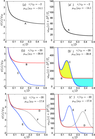
Figure 1: (Color online) Normalized 1d profiles $\psi(z)/\psi_{D}$ (left) and $\omega_{\rm{loc}}(z)D^{3}/T_{c}$ (right) vs $z/D$ for $(\tau/\tau_{D},\mu_{\infty}/\mu_{D})=(-2,-14.1)$ (top), $(-20,-30.8)$ (middle), and $(-20,-17.8)$ (bottom). Top: Adsorption-dominated profile A with $\psi(z)>0$. Middle: Two profiles B and C on the capillary condensation line with the same grand potential $\Omega$. In (b’), the two curves of $\omega_{\rm{loc}}(z)$ enclose two regions with the same area close to the surface tension $\sigma$. Bottom: Three profiles D,E, and F with the same $\tau$ and $\mu_{\infty}$ (see Fig.3). In (c’), $\Omega$ increases in the order of D, E, and F.

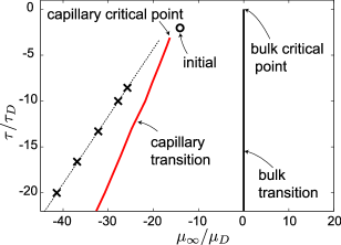
Figure 2: (Color online) Phase diagram of a near-critical fluid in a film for large adsorption in the $\mu_{\infty}/\mu_{D}$- $\tau/\tau_{D}$ plane. The bulk coexistence line is given by $\tau<0$ and $\mu_{\infty}=0$. On its left, there appears a first-order capillary condensation line (red bold line) ending at a film critical point, which is calculated from 1d profiles. Displayed also are values of $\mu_{\infty}/\mu_{D}$ in steady two-phase coexistence in our simulation of a $2D\times 2D\times D$ system ($\times$). Starting point of our simulation ($t<0$) is also shown ($\circ$).

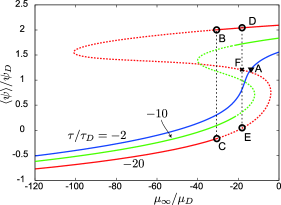
Figure 3: (Color online) Isothermal curves in the $\mu_{\infty}/\mu_{D}$-$\langle{\psi}\rangle/\psi_{D}$ plane, which are calculated for 1d profiles at $\tau/\tau_{D}=-2$, -10, and -20. For $\tau$ less than its film critical value ($=-3.14\tau_{D}$), a van der Waals loop appears. Dotted parts of the curves for $\tau/\tau_{D}=-10$ and -20 are not stable in contact with a reservoir. Points A,B,C,D,E, and F correspond to the curves in Fig.1.

We suppose a near-critical fluid between parallel symmetric walls in the region $0<z<D$, where $D$ is much longer than any microscopic lengths. To avoid the discussion of the edge effect, the lateral plate dimension $L$ is supposed to much exceed $D$. The fluid is close to the bulk criticality and above the prewetting transition line Evansreview ; Cahn ; PG ; Bonn . We use our local functional theory, neglecting the two-dimensional thermal fluctuations with sizes exceeding $D$ in the $xy$ plane.

We scale $\tau$ and $\psi$ in units of $\tau_{D}\propto D^{-1/\nu}$ and $\psi_{D}\propto D^{-\beta/\nu}$, respectively, defined by

$$\tau_{D} = (\xi_{0}/D)^{1/\nu},$$ (2.18)

$$\psi_{D} = (24^{\beta/\nu}/3u^{*}C_{1}\xi_{0})^{1/2}\tau_{D}^{\beta}.$$ (2.19)

In equilibrium theory, it is convenient to assume that the fluid between the walls is in contact with a large reservoir containing the same binary mixture, where the order parameter is $\psi_{\infty}$ and the chemical potential is

$$\mu_{\infty}=\mu(\psi_{\infty},\tau).$$ (2.20)

Here, $\mu_{\infty}$ corresponds to magnetic field $h$ for films of Ising spin systems. We are interested in the case $\mu_{\infty}<0$ (or $\psi_{\infty}<0$) and $\psi_{0}>0$, where $\psi_{0}$ is the value of $\psi$ at the walls. If equilibrium is attained in the total system including the reservoir, we should minimize the film grand potential $\Omega$. Including the surface free energy, we assume the form,

$$\Omega=\int d{\mbox{\boldmath$r$}}~{}\omega_{\rm{loc}}-T_{c}\int dS~{}h_{1}\psi,$$ (2.21)

where the space integral $\int d{\mbox{\boldmath$r$}}$ is within the film, the surface integral $\int dS$ is on the walls at $z=0$ and $D$, and $h_{1}$ is a surface field symmetrically given on the two walls. In addition, we neglect the surface free energy of the form $\int dS\lambda^{-1}\psi^{2}$ assumed in the literatureCahn ; Bonn ; Binderreview ; PG (or we consider the limit $\lambda\to\infty$).

In Eq.(2.21) $\omega_{\rm{loc}}$ is the local grand potential density including the gradient part,

$$\omega_{\rm{loc}}=\omega_{s}+\frac{1}{2}T_{c}C|\nabla\psi|^{2},$$ (2.22)

where $\omega_{s}$ is the excess grand potential density written as

$$\omega_{s}=f(\psi)-f(\psi_{\infty})-\mu_{\infty}(\psi-\psi_{\infty}).$$ (2.23)

Now minimization of $\Omega$ yields the bulk equation,

$$\frac{\delta F}{\delta\psi}=\mu-\frac{T_{c}}{2}C^{\prime}|\nabla\psi|^{2}-T_{c}C\nabla^{2}\psi=\mu_{\infty},$$ (2.24)

where $C^{\prime}=\partial C/\partial\psi$. The boundary conditions at $z=0$ and $D$ are given by

$$\psi^{\prime}(x,y,0)=-\psi^{\prime}(x,y,D)=-h_{1}/C.$$ (2.25)

where $\psi^{\prime}=\partial\psi/\partial z$.

The role of $h_{1}$ in this paper is simply to assure the strong adsorption regime $\psi_{0}/|\tau|^{\beta}\gg(C_{1}\xi_{0})^{-1/2}$ Liu ; Yang ; Oka , where $\psi_{0}$ is the boundary value of $\psi$. This regime is eventually realized on approaching the criticality (however small $h_{1}$ is). In our simulation, the profile of $\psi$ in the region $0<z<\xi$ is nearly one-dimensional depending only on $z$ even in two phase states (see Figs.5 and 6). It decays slowly as $(\ell_{0}+z)^{-\beta/\nu}$ for $0<z<\xi$ Liu ; Lawreview ; Rudnick ; Oka , where $\ell_{0}$ is a short microscopic length introduced by Rudnick and Jasnow Rudnick . With the gradient free energy in the form of Eq.(2.22), $\ell_{0}$ is expressed as

$$\ell_{0}\sim\xi_{0}(C_{1}\xi_{0})^{-\nu/2\beta}\psi_{0}^{-\nu/\beta}\sim D(\psi_{D}/\psi_{0})^{-\nu/\beta},$$ (2.26)

in terms of $\psi_{0}$. The excess surface adsorption of $\psi$ in the region $0<z<\ell_{0}$ is of order $\psi_{0}\ell_{0}\sim\psi_{0}^{1-\nu/\beta}$ and is negligible for large $\psi_{0}$ from $\beta/\nu\sim 2$, while that in the region $\ell_{0}<z<\xi$ is of order $\xi^{1-\beta/\nu}$ for $\xi(\tau,\psi_{m})<D/2$ Liu ; Rudnick ; Lawreview . In the strong-adsorption regime we calculate the average of $\psi$ along the $z$ axis,

$$\langle{\psi}\rangle=\int_{0}^{D}dz\psi/D.$$ (2.27)

In two-phase states, $\langle{\psi}\rangle$ depends on $(x,y)$.

From Eq.(2.25) it follows the estimation $h_{1}\sim C(\psi_{0})\psi_{0}/\ell_{0}$. As $h_{1}/|\tau|^{\beta\delta-\nu}\to\infty$, we find

$$h_{1}=\psi_{0}^{\delta-\nu/\beta}(B_{1}+B_{2}\tau\psi_{0}^{-1/\beta}+\cdots),$$ (2.28)

where $B_{1}$ and $B_{2}$ are positive constants. This is the expression for $D\to\infty$. In this regime, the surface free energy in Eq.(2.21) is given by $-2B_{1}\psi_{0}^{2\nu/\beta}A$, where $A=L^{2}$ is the surface area. In our previous paperOka , we examined the film phase behavior at fixed large $\psi_{0}$, treating the surface free energy as a constant. In our simulation, we assume the boundary condition (2.25) with $h_{1}/C=1011\psi_{D}/D$ to obtain $\psi_{0}/\psi_{D}\cong 14.8$.

II.5 Capillary condensation transition

We consider the capillary condensation transition on the basis of one-dimensional (1d) profiles $\psi=\psi(z)$. From Eq.(2.25), we have the symmetry $\psi(z)=\psi(D-z)$. In the region $0<z<D/2$, Eq.(2.24) is integrated to give

$$z=\int^{\psi_{0}}_{\psi}d\psi\bigg{[}\frac{C(\psi)/2}{\omega_{s}(\psi)+\Pi}\bigg{]}^{1/2}.$$ (2.29)

Here, $\Pi=-{A^{-1}}{\partial\Omega}/{\partial D}$ is the osmotic pressure. It is the force density per unit area exerted by the fluid to the plates. In our case, $\Pi<0$, indicating attractive inter-wall interaction. In the 1d case, it is also written as

$$\Pi = f(\psi_{\infty})-f(\psi_{m})-\mu_{\infty}(\psi_{\infty}-\psi_{m})$$ (2.30)

$$= -\omega_{s}(\psi_{m}).$$

At the midpoint $z=D/2$, we set $\psi_{m}=\psi(D/2)$. The fluid at the midpoint can be in the phase favored by the walls with $\psi_{m}\sim\psi_{\rm cx}$ due to the strong adsorption on the walls or in the disfavored phase with $\psi_{m}\cong\psi_{\infty}<0$. Equation (2.30) indicates $\Pi\cong 2\mu_{\infty}\psi_{\rm cx}$ in the former case and $\Pi\cong-T_{c}(\psi_{m}-\psi_{\infty})^{2}/2\chi_{\rm cx}\cong 0$ in the latter case, so $\Pi$ can be very different in these two cases comment2 .

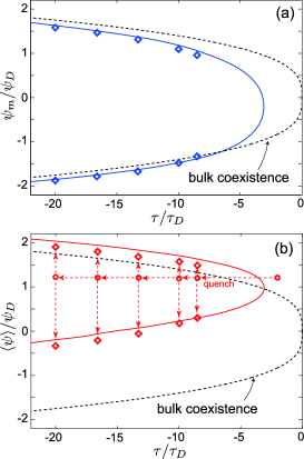
Figure 4: (Color online) Phase diagrams in the $\tau/\tau_{D}$-${\psi_{m}}/\psi_{D}$ plane in (a) and in the $\tau/\tau_{D}$-$\langle{\psi}\rangle/\psi_{D}$ plane in (b), where $\psi_{m}$ is the midpoint value. In (a) and (b), the capillary condensation curves (bold lines) are calculated from 1d profiles, where points for five $\tau/\tau_{D}$ are those along the $z$ axis with $(x,y)=(D,D)$ and $(D,0)$ in the final two-phase states in our simulation (see Figs.4 and 5). Bulk coexistence curve is in broken line. In (b) our phase separation process is illustrated by arrows, where the total order parameter is conserved.

Figure 1 displays typical 1d profiles of $\psi(z)$ from Eq.(2.29) and $\omega_{\rm{loc}}(z)$ in Eq.(2.22) in the range $0<z<D/2$, which will be needed to explain our simulation results. Here we set $(\tau/\tau_{D},\psi_{\infty}/\psi_{D},\mu_{\infty}/\mu_{D})=(-2,-1.14,-14.1)$ (top), $(-20,-1.85,-30.8)$ (middle), and $(-20,-1.81,-17.8)$ (bottom), where $\mu_{\infty}$ is measured in units of

$$\mu_{D}=T_{c}/D^{3}\psi_{D}\propto D^{\nu/\beta-3}.$$ (2.31)

Salient features in Fig.1 are as follows. (i) In Fig.1(a), $\psi$ is positive in the whole region with $<\psi>/\psi_{D}=1.20$. (ii) In Figs.1(b) and (b’), the fluid is on the capillary condensation line, where we give two equilibrium profiles B and C with the same $\Omega$. Here, B represents an adsorption-dominated state with $\psi_{m}\sim\psi_{\rm cx}$ and $<\psi>/\psi_{D}=1.99$, while for C the film center is occupied by the disfavored phase with $\psi_{m}\sim-\psi_{\rm cx}$ and $<\psi>/\psi_{D}=0.187$. In the right panel (b’), the integral of $\omega_{\rm{loc}}(z)$ in the region $0<z<D/2$ is the same for B and C. The enclosed two regions have the same area $24.7$ in units of $T_{c}/D^{2}$, which is close to the surface tension $\sigma=29.2T_{c}/D^{2}$ at this $\tau$. In addition, $\Pi\sim-\sigma/D$ for B and $\Pi\cong 0$ for C comment2 . (iii) In Figs.1(c) and (c’), the parameters are those slightly below the capillary condensation line (in Fig.2 below). Here, there are three solutions with the common $\tau$ and $\mu_{\infty}$, but $<\psi>/\psi_{D}$ is $2.03$ for (D), 0.028 for (E), and 1.20 for (F) (see Fig.3 below). If we perform simulation in contact with a reservoir with these $\tau$ and $\mu_{\infty}$, the profile D is realized at long times. In the very early stage of our simulation, the dynamics is one-dimensional and the profile F is approached after quenching from A in Fig.1(a) (see Fig.7 below).

In Fig.2, we show the capillary condensation line (CCL) from 1d profiles located on the left of the bulk coexistence line in the $\tau$-$\mu_{\infty}$ plane. In our previous paper Oka , the corresponding phase diagram was displayed in the $\tau$-$\psi_{\infty}$ plane. The discontinuities of the physical quantities across CCL increase with increasing $|\tau|$ vanishing at a film critical point. At this film criticality, $\tau$, $\psi_{\infty}$, and $\mu_{\infty}$ are calculated as

$$\bigg{(}\frac{\tau}{\tau_{D}},\frac{\psi_{\infty}}{\psi_{D}},\frac{\mu_{\infty}}{\mu_{D}}\bigg{)}=(-3.14,-1.27,-16.3),$$ (2.32)

where we also have $\langle{\psi}\rangle/\psi_{D}=0.989$ and $\psi_{m}/\psi_{D}=-0.173$. Hereafter, the chemical potential $\mu_{\infty}$ on this CCL will be written as $\mu_{\rm cx}^{\rm ca}(\tau)$. Our numerically calculated CCL is well fitted to the linear form,

$$\mu_{\rm cx}^{\rm ca}(\tau)/\mu_{D}+16.3\cong 0.86(\tau/\tau_{D}+3.14).$$ (2.33)

In Fig.1(b’), the two areas enclosed by the two curves of $\omega_{\rm loc}D^{3}/T_{c}$ are the same ($\sim\sigma D^{2}/T_{c}$). Thus, for $|\tau|/\tau_{D}\gg 1$, the surface tension $\sigma$ and the free energy difference per unit area $-2\mu_{\rm cx}^{\rm ca}\psi_{\rm cx}D$ are of the same order. See the sentences below Eq.(2.30) and the explanation of Fig.1(b’). For $|\tau|\gg\tau_{D}$, it follows the relation,

$$\mu_{\rm cx}^{\rm ca}\sim-\sigma/\psi_{\rm cx}D\sim-|\tau/\tau_{D}|^{2\nu-\beta}\mu_{D}.$$ (2.34)

Since $2\nu-\beta\cong 0.94$, the theoretical formula (2.34) is consistent with the numerical formula (2.33). Note that Eq.(2.34) is equivalent to the Kelvin equation known for the gas-liquid transition in pores Evansreview ; Gelb .

We have already presented a special case of three 1d profiles in Fig.1(c) for $(\tau/\tau_{D},\mu_{\infty}/\mu_{D})=(-20,-17.8)$. In Fig.3, we show isothermal curves in the $\mu_{\infty}$-$\langle{\psi}\rangle$ plane, which are calculated from 1d profiles with $\tau/\tau_{D}=-2$, $-10$, and $-20$. The relation between $\mu_{\infty}$ and $\langle{\psi}\rangle$ is monotonic for $\tau/\tau_{D}\geq-3.14$ (above the film critical temperature), while it exhibits a van der Waals loop for $\tau/\tau_{D}<-3.14$ with three 1d states in a window range $\mu_{\infty 1}<\mu_{\infty}<\mu_{\infty 2}$ comment3 . Here, $\mu_{\infty 1}$ and $\mu_{\infty 2}$ coincide at the film criticality. The isothems consist of stable and unstable parts characterized by the sign of the film susceptibility defined by

$$\chi_{\rm film}=T_{c}(\partial\langle{\psi}\rangle/\partial\mu_{\infty})_{\tau}.$$ (2.35)

In Fig,3, points A,B,C,D,E, and F correspond to the curves in Fig.1. Dotted parts of the two curves of $\tau/\tau_{D}=-10$ and $-20$ are not stable in the presence of a mass current from a reservoir with common $\mu_{\infty}$.

Previously, some authors p ; Binder-Landau calculated the stable parts of isotherms of the average density in the film versus the chemical potential. In our local functional theory, the three 1d profiles can be calculated since a unique profile follows for any given set of $\tau$ and $\langle{\psi}\rangle$. In equilibrium fluctuation theory of films Evansreview , $\chi_{\rm film}$ is proportional to the variance of the order parameter fluctuations, so its negativity indicates thermodynamic instability.

Furthermore, Fig.4 gives the phase diagrams in the $\tau$-${\psi_{m}}$ and $\tau$-${\langle{\psi}\rangle}$ planes. Bold lines represent the capillary condensation curve from 1d profiles as in Fig.2. In steady two-phase states in our simulation, $\psi_{m}$ and $\langle{\psi}\rangle$ depend on $x$ and $y$, so points for five $\tau$ represent $\psi_{m}(x,y)=\psi(x,y,D/2)$ and $\langle{\psi}\rangle(x,y)$ with $(x,y)=(D,D)$ and $(D,0)$ (see Figs.5 and 6). The former line passes through a domain of the phase disfavored by the walls and the latter through the favored phase only. Phase diagrams similar to Fig.4(b) have been obtained in experiments of the capillary condensation in porous media Gelb .

Table 1: Values of $\mu_{\infty}/\mu_{D}$ from our simulation in a finite $2D\times 2D\times D$ system for five $\tau/\tau_{D}$. The corresponding values of $\mu_{\rm cx}^{\rm ca}/\mu_{D}$ on the CCL from 1d profiles are also shown.

$\tau/\tau_{D}$	$-8.5$	$-10$	$-13.3$	$-16.6$	$-20$
$\mu_{\infty}/\mu_{D}$ (finite)	-25.8	-27.8	-32.2	-36.6	-41.4
$\mu_{\rm cx}^{\rm ca}/\mu_{D}$ (1d)	-20.6	-21.8	-24.9	-27.7	-30.8

III Phase separation dynamics

We performed simulation of phase separation in a $L\times L\times D$ cell with $L=2D$ imposing the periodic boundary condition along the $x$ and $y$ axes. In this section, we describe phase separation realized for deep quenching. However, it was not realized for shallow quenching $(|\tau|/\tau_{D}\lesssim 7$), for which $\chi_{\rm film}$ in Eq.(2.35) is positive.

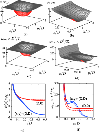
Figure 5: (Color online) Equilibrium two-phase state at $\tau/\tau_{D}=-10$ in a $2D\times 2D\times D$ system: $\psi/\psi_{D}$ (top) and $\omega_{\rm loc}D^{3}/T_{c}$ (middle) in the $xy$ plane at $z=D/2$ (left) and in the $yz$ plane at $x=D$ (right). Bottom: $\psi/\psi_{D}$ (left) and $\omega_{\rm loc}D^{3}/T_{c}$ (right) along the $z$ axis for $(x,y)=(D,D)$ (blue bold line) and $(D,0)$ (red bold line), while dotted lines represent 1d profiles from Eq.(2.29).

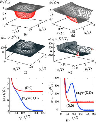
Figure 6: (Color online) Equilibrium two-phase state at $\tau/\tau_{D}=-20$ in a $2D\times 2D\times D$ system: $\psi/\psi_{D}$ (top) and $\omega_{\rm loc}D^{3}/T_{c}$ (middle) in the $xy$ plane at $z=D/2$ (left) and in the $yz$ plane at $x=D$ (right). Bottom: $\psi/\psi_{D}$ (left) and $\omega_{\rm loc}D^{3}/T_{c}$ (right) along the $z$ axis for $(x,y)=(D,D)$ (blue bold line) and $(D,0)$ (red bold line), which are closer to the 1d profiles (dotted lines) from Eq.(2.29) than in Fig.5.

III.1 Dynamic equations and simulation method

Supposing an incompressible fluid binary mixture with a homogeneous temperature, we use the model H equations H77 ; Kawasaki-Ohta ; Onukibook . The order parameter $\psi$ is a conserved variable governed by

$$\frac{\partial\psi}{\partial t}=-\nabla\cdot(\psi{\mbox{\boldmath$v$}})+\lambda\nabla^{2}\frac{\delta F}{\delta\psi},$$ (3.1)

where $\lambda$ is the kinetic coefficient and the functional derivative ${\delta F}/{\delta\psi}$ may be calculated from Eq.(2.4) with the aid of Eqs.(2.10), (2.15), and (2.16) outside and inside CX. We neglect the random source term originally present in critical dynamics H77 ; Onukibook , because we treat the deviations much larger than the thermal fluctuations. The velocity field $v$ satisfies $\nabla\cdot{\mbox{\boldmath$v$}}=0$ and vanishes at $z=0$ and $D$. In the Stokes approximationKawasaki-Ohta , $v$ is determined by

$$\bar{\eta}\nabla^{2}{\mbox{\boldmath$v$}}=\nabla p_{0}+\psi\nabla(\delta F/\delta\psi),$$ (3.2)

where $\bar{\eta}$ is the shear viscosity and the role of a pressure $p_{0}$ is to ensure $\nabla\cdot{\mbox{\boldmath$v$}}=0$. See Appendix for the expression of the stress tensor in near-critical fluids and the derivation of Eq.(3.2).

The kinetic coefficients $\lambda$ and $\bar{\eta}$ should be treated as renormalized ones H77 ; Kawasaki-Ohta ; Onukibook (see the last sentence of Subsec.IIA). In the vicinity of the bulk coexistence curve, $\lambda$ may be approximated by

$$\lambda=\chi_{\rm cx}D_{\xi}/T_{c},$$ (3.3)

where $\chi_{\rm cx}$ is the susceptibility on CX in Eq.(2.13) and $D_{\xi}$ is the mutual diffusion constant of the Stokes form,

$$D_{\xi}=T_{c}/6\pi\bar{\eta}\xi,$$ (3.4)

with $\xi=\xi_{0}^{\prime}|\tau|^{-\nu}$ being the correlation length on CX. In our simulation, $|\psi|$ is of order $\psi_{\rm cx}$ at $z=D/2$ (see Figs.5 and 6 below), which supports Eqs.(3.3) and (3.4). The viscosity $\bar{\eta}$ exhibits a very weak critical singularity and may be treated as a constant independent of $\tau$.

In this paper, we also performed simulation for model B without the hydrodynamic interaction H77 , where $\psi$ obeys the diffusive equation,

$$\frac{\partial\psi}{\partial t}=\lambda\nabla^{2}\frac{\delta F}{\delta\psi}.$$ (3.5)

The kinetic coefficient $\lambda$ is assumed to be given by Eqs.(3.3) and (3.4) as in the model H case. Then, comparing the results from the two models, we can examine the role of the hydrodynamic interaction in phase separation. Model B has been used to investigate surface-directed phase separation in binary alloys Das .

In integrating Eqs.(3.1) and (3.5), the mesh length was $\Delta x=D/32$ and the time interval width was $\Delta t=2\times 10^{-6}t_{0}$. The initial state was the 1d profile A in Fig.1(a) at $\tau/\tau_{D}=-2$ with small random numbers ($\sim 10^{-4}$) superimposed at the mesh points. At $t=0$, we decreased $\tau$ to a final reduced temperature. For $t>0$, there was no mass exchange between the film and the reservoir so that the total order parameter $\int d{\mbox{\boldmath$r$}}\psi$ was fixed at $1.20\psi_{D}DL^{2}$. We will measure time after quenching in units of

$$t_{0}=D^{2}/D_{\xi},$$ (3.6)

which is the mutual diffusion time in the film assumed to be much longer than the thermal diffusion time. We note that the natural time unit in bulk phase separation has been the order parameter relaxation time $t_{\xi}=\xi^{2}/D_{\xi}$ Kawasaki-Ohta ; Siggia ; Onukibook . Here, $t_{0}/t_{\xi}=(D/\xi)^{2}=R_{\xi}^{2}|\tau/\tau_{D}|^{2\nu}\sim 100$ for $|\tau/\tau_{D}|\sim 10$.

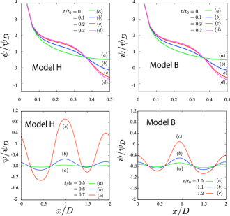
Figure 7: (Color online) Early-stage time-evolution of $\psi/\psi_{D}$ for model H (left) and model B (right) after quenching from the profile A in Fig.1(a) to $\tau/\tau_{D}=-20$. Shown are the profiles along the $z$ axis for $(x,y)=(D,D)$ at $t/t_{0}=0$, 0.1, 0.2, and 0.3 (top) and along the $x$ axis for $(y,z)=(1.5D,0.5D)$ (bottom) at later times. In the top panels, the profile F in Fig.1(c) is approached without noticeable differences between the two models. In the bottom panels, fluctuations in the $xy$ plane appear and coarsening is much quickened for model H than for model B, where $t/t_{0}=$ 0.5, 0.6, and 0.7 for model H and 1.0, 1.1, and 1.2 for model B.

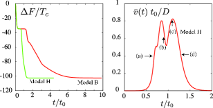
Figure 8: (Color online) Time-evolution of the normalized free energy decrease $\Delta F(t)/T_{c}$ for model H and model B (left) and $\bar{v}(t)t_{0}/D$ for model H (right) after quenching from the profile A in Fig.1(a). At points (a), (b), (c), and (d) (right) snapshots of $\psi$ and $v$ will be given in Fig.9.

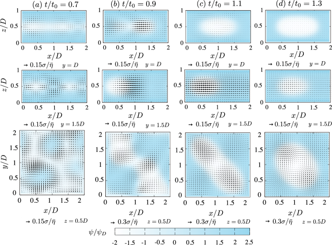
Figure 9: (Color online) Cross-sectional velocity field $v$ (arrows) and order parameter $\psi$ (in gradation according the color bar) in phase separation for $\tau/\tau_{D}=-20$ in model H, where $t/t_{0}$ is equal to (a) 0.7, (b) 0.9, (c) 1.1, and (d) 1.3 after quenching. Displayed are $(v_{x},v_{z})$ and $\psi$ in the $xz$ plane at $y=D$ (top), those at $y=1.5D$ (middle), and $(v_{x},v_{y})$ and $\psi$ in the $xy$ plane at $z=D/2$ (bottom). Arrows below panels indicate typical magnitudes of the velocities, where $\sigma$ is the surface tension and $\bar{\eta}$ is the shear viscosity. Final state is given in Fig.6.

III.2 Steady two-phase states

For sufficiently deep quenching, we realized phase separation to find a steady two-phase state at long times both for model H and model B. We could also calculate this final state more accurately from the following relaxation-type equation,

$$\frac{\partial\psi}{\partial t}=-L_{0}\bigg{[}\frac{\delta F}{\delta\psi}-\bigg{\langle}{\frac{\delta F}{\delta\psi}}\bigg{\rangle}_{t}\bigg{]},$$ (3.7)

where $L_{0}$ is a constant and $\langle{{\delta F}/{\delta\psi}}\rangle_{t}$ is the space average of ${\delta F}{\delta\psi}$ at time $t$. Because of its simplicity, we integrated Eq.(3.7) with a fine mesh length of $\Delta x=D/64$. The data points in Figs.2 and 4 and the snapshots in Figs.5 and 6 are those from the steady states of Eq.(3.7).

In Fig.4, the deviations of $\psi_{m}$ and $\langle{\psi}\rangle$ from those on CCL are surprisingly small, though the lateral dimension $L$ is only $2D$. However, in Table 1, the final two-phase values of $\mu_{\infty}$ considerably deviate from those on CCL. This may be ascribed to the relatively small size of the susceptibility $\chi_{\rm cx}$ for these cases. That is, if we set $\chi_{\rm cx}=A_{\chi}^{-1}T_{c}\psi_{D}/\mu_{D}$ on CX, we obtain $A_{\chi}=120$ and 283 for $\tau/\tau_{D}=-10$ and $-20$, respectively. Here, if we multiply the deviation of ${\psi_{m}}/\psi_{D}$ or $\langle{\psi}\rangle/\psi_{D}$ by of $A_{\chi}$, we obtain that of $\mu_{\infty}/\mu_{D}$.

In Figs.5 and 6, we display the final profiles of $\psi$ and $\omega_{\rm loc}$ in the $xy$ plane at $z=D/2$ (left) and in the $zy$ plane at $x=D$ (right) for $\tau/\tau_{D}=-10$ and $-20$. In these cases, $\xi$ on CX is $0.078D$ and $0.051D$, respectively, which is of the order of the interface thickness. Displayed in the bottom panels are 1d profiles of $\psi$ and $\omega_{\rm loc}$ along the $z$ axis for the two lateral points $(x,y)=(D,D)$ and $(D,0)$. These profiles are rather close to the 1d profiles from Eq.(2.29) in accord with Fig.4.

III.3 Time evolution

Both for model H and model B, early-stage time-evolution proceeds as follows. Just after quenching, $\psi$ changes only along the $z$ axis to approach the 1d profile at the final $\tau$ with fixed $\langle{\psi}\rangle$ (see Fig.3). If this 1d profile satisfies the instability condition $\chi_{\rm film}<0$, it follows 3d spinodal decomposition. On the other hand, if it satisfies the stability condition $\chi_{\rm film}>0$, it remains stationary in simulation without thermal noise.

Figure 7 displays $\psi$ after quenching to $\tau/\tau_{D}=-20$. In the top panels, it is plotted along the $z$ axis with $(x,y)=(D,D)$ at $t/t_{0}=0,0.1,0.2,$ and 0.3. The velocity field nearly vanishes for model H, so there is almost no difference between the results of these models. However, in the bottom panels, the 1d profile becomes unstable with respect to the fluctuations varying in the $xy$ plane for $t/t_{0}\gtrsim 0.5$. The velocity field grows gradually for model H. In this second time range, the domain formation is much quicker for model H than for model B.

In the left panel of Fig.8, we show the free energy decrease $\Delta F=F(t)-F(+0)$ at $\tau/\tau_{D}=-20$ as a function of $t$ for model H and model B. Here, $F(t)$ is the total bulk free energy in Eq.(2.4) with $F(+0)$ being its value just after quenching. Its decrease is accelerated with development of the fluctuations in the $xy$ plane. The coarsening is slower for model B than for model H by about 5 times. In the right panel of Fig.8, we show the characteristic velocity amplitude ${\bar{v}}(t)$ for model H, which is defined by

$${\bar{v}}(t)^{2}=\int d{\mbox{\boldmath$r$}}|{\mbox{\boldmath$v$}}|^{2}/DL^{2}.$$ (3.8)

For $\tau/\tau_{D}=-20$, ${\bar{v}}(t)$ is equal to 0.021, 0.106, and 0.485 at $t/t_{0}=0.5$, 0.6, and 0.7, respectively, increasing up to $0.8$, in units of $D/t_{0}$.

In Fig.9, we show late stage snapshots of $\psi$ and $v$ in the $xz$ plane (top) and in the $xy$ plane (middle) for $\tau/\tau_{D}=-20$ for model H, where $t/t_{0}$ is equal to (a) 0.7, (b) 0.9, (c) 1.1, and (d) 1.3 after quenching. In (a) we can see a network-like domain of the disfavored phase. In (b) three domains can be seen, where the middle one is being absorbed into the bottom one, soon resulting in two domains at $t/t_{0}\sim 1.0$. This process gives rise to a dip in ${\bar{v}}(t)$ in Fig.8(b) since these two domains are considerably apart. In (c) and (d), furthermore, coalescence of these two domains is taking place. The arrows below the panels indicate the typical velocity, $0.15\sigma/\bar{\eta}$ or $0.3\sigma/\bar{\eta}$, where $\sigma$ is the surface tension and $\bar{\eta}$ is the shear viscosity. Note that the typical velocity in the late-stage bulk spinodal decomposition is given by $v_{c}=0.1\sigma/\bar{\eta}$ Siggia ; Onukibook , which follows from the stress balance $\sigma/R\sim 6\pi{\bar{\eta}}v_{c}/R$ with $R\sim v_{c}t$ being the typical domain length. In our case, from Eq.(2.17) these velocities are related as

$$D/t_{0}=T_{c}/6\pi{\bar{\eta}}\xi D=(\xi/6\pi A_{\sigma}D)(\sigma/{\bar{\eta}}).$$ (3.9)

Thus, $D/t_{0}=0.036\sigma/\bar{\eta}$ for $\tau/\tau_{D}=-20$ in Fig.9.

IV Summary and remarks

In summary, we have examined the phase separation in a near-critical binary mixture between symmetric parallel plates in the strong adsorption regime around the capillary condensation line (CCL). Using model H and model B, simulation has been performed in a $2D\times 2D\times D$ cell. We summarize our main results.
(i) In Sec.II, we have presented the singular free energy with the gradient part outside and inside the bulk coexistence curve. Applying it to near-critical fluids between parallel plates, typical 1d profiles have been given in Fig.1. CCL has been plotted in the $\tau$-$\mu_{\infty}$ plane in Fig.2. The points for the steady two-phase states from our simulation are located in the left side of CCL. In Fig.3, we have also found the van der Waals loop of isothermal curves in the $\langle{\psi}\rangle$-$\mu_{\infty}$ plane, where $\tau$ is smaller than the film critical value. The phase diagrams have been plotted in the $\tau$-$\psi_{m}$ and $\tau$-$\langle{\psi}\rangle$ planes in 3d (bulk) and 2d (film) in Fig.4. The Kelvin relation (2.34) has also been obtained, since the osmotic pressure $\Pi$ is of order $-\sigma/D$ right below CCL comment2 .
(ii) In Sec.III, we have first displayed the cross-sectional profiles of $\psi$ and $\omega_{\rm loc}$ in steady two-phase states in Figs.5 and 6. The profiles along $z$ axis for $(x,y)=(D,D)$ and $(D,0)$ closely resemble the corresponding 1d profiles. For quenching to $\tau/\tau_{D}=-20$, we have examined time-evolution of $\psi$. It occurs only along the $z$ axis in the very early stage in the top panels of Fig.7, where there is no difference between the results of model H and model B. Subsequently, inhomogeneities appear in the $xy$ plane. The free energy decrease $\Delta F(t)=F(t)-F(+0)$ and the typical velocity amplitude ${\bar{v}}(t)$ defined in Eq.(3.8) have been plotted in Fig.8. The velocity field considerably quicken the interface formation and the coarsening for model H than for model B. Profiles of $\psi$ and $v$ in the late stage coarsening due to the flow have been presented in Fig.9, where the domain coalescence can be seen and the maximum velocity is of order $0.1\sigma/{\bar{\eta}}$ as in bulk spinodal decomposition Siggia .

We make some remarks.
1) In the static part of our theory, we neglect the thermal fluctuations varying in the lateral directions with wavelengths longer than $D$. Thus this 2d transition exhibits mean-field behavior. In fact, the curves of $\psi_{m}$ vs $\tau$ and $\langle{\psi}\rangle$ vs $\tau$ are parabolic near the film criticality in Fig.4.
2) In our simulation, we soon have only two or three domains in the cell as in the bottom panels of Fig.9. The lateral dimension $L=2D$ in this paper is too short to investigate the domain growth law in the $xy$ plane. Simulation with larger $L/D$ should be performed in future.
3) From the van der Waals loop of the isothermal curves in the $\langle{\psi}\rangle$-$\mu_{\infty}$ plane in Fig.3, we may predict how phase separation proceeds after quenching. We have examined phase separation via spinodal decomposition. However, in real experiments, phase separation may occur via nucleation for metastable 1d profiles. Note that hysteretic behavior has been observed in phase-separating fluids in pores and has not been well explained Evansreview ; Gelb ; Goldburg ; Wil .
4) In a number of experiments and simulations of surface-directed phase separation Araki ; Bates ; Puri , composition waves along the $z$ axis have been observed near the wall in the early stage. In these cases, the degree of adsorption has changed appreciably upon quenching. In the strong adsorption regime in this paper, 1d dynamics occurs in the initial stage, but there are no composition waves as in the top panels of Fig.7.
5) The static part of this work is applicable to any Ising-like near-critical systems and can readily be generalized to $n$-component spin systems. In the dynamics, we have used model H with a homogeneous temperature and incompressible flows. On the other hand, in one-component near-critical fluids, the latent heat released or absorbed at the interfaces gives rise to significant hydrodynamic flow because of the enhanced isobaric thermal expansion Onukibook ; Teshi . Also promising in future should be extension of this work to near-critical fluids in porous media.

Appendix: Stress tensor in near-critical fluids

In near-critical fluids, we treat slow flows with low Reynolds numbers. The total (reversible) stress tensor is given by $p_{0}\delta_{ij}+\Pi_{\psi ij}$, where $p_{0}$ is nearly homogeneous throughout the film and the reservoir. The $\Pi_{\psi ij}$ is the stress tensor due to the composition deviationOnukibook ,

$$\Pi_{\psi ij}=p_{\psi}\delta_{ij}+C(\nabla_{i}\psi)(\nabla_{j}\psi),$$ (A1)

where $\nabla_{i}=\partial/\partial x_{i}$. The diagonal part $p_{\psi}$ is written as

$$p_{\psi} = \psi\mu-f-\frac{1}{2}(C+C^{\prime}\psi)|\nabla\psi|^{2}-C\psi\nabla^{2}\psi$$ (A2)

$$= \psi(\delta F/\delta\psi)-f-C|\nabla\psi|^{2}/2,$$

where $C^{\prime}=\partial C/\partial\phi$. The second part in Eq.(A1) contains off-diagonal components relevant for curved interfaces. In deriving Eq.(3.2), we use the relation,

$$\sum_{j}\nabla_{j}\Pi_{\psi ij}=\psi\nabla_{i}(\delta F/\delta\psi).$$ (A3)

References

- (1) R. Evans and U. M. B. Marconi, J. Chem. Phys. 86, 7138 (1987); R. Evans, J. Phys.: Condens. Matter 2, 8989 (1990).
- (2) L.D. Gelb, K.E. Gubbins, R. Radhakrishnan, and M. Sliwinska-Bartkowiak, Rep. Prog. Phys. 62, 1573 (1999).
- (3) K. Binder, D. Landau, and M. Mller, J. Stat. Phys. 110, 1411 (2003); M. Mller and K. Binder, J. Phys.: Condens. Matter 17, S333 (2005); K.Binder, J. Horbach, R. Vink, and A. De Virgiliis, Soft Matter, 4, 1555 (2008).
- (4) J. W. Cahn, J. Chem. Phys. 66 3667 (1977).
- (5) K. Binder, in Phase Transitions and Critical Phenomena, C. Domb and J. L. Lebowitz, eds. (Academic, London, 1983), Vol. 8, p. 1.
- (6) P.G. de Gennes, Rev. Mod. Phys. 57, 827 (1985).
- (7) D. Bonn and D. Ross, Rep. Prog. Phys. 64, 1085 (2001).
- (8) B. M. Law, Prog. Surf. Sci. 66, 159 (2001).
- (9) J. Rudnick and D. Jasnow, Phys. Rev. Lett. 48, 1059 (1982); ibid. 49, 1595 (1982)
- (10) A. J. Liu and M. E. Fisher, Phys. Rev. A 40, 7202 (1989).
- (11) M. E. Fisher and H. Nakanishi, J. Chem. Phys. 75, 5857 (1981); H. Nakanishi and M. E. Fisher, J. Chem. Phys. 78, 3279 (1983).
- (12) R. Evans, U. M. B. Marconi, P. Tarazona, J. Chem. Soc.,Faraday. Trans. 82, 1763 (1986); P. Tarazona, U.M.B Marconi, R. Evans, Mol. Phys. 60, 573 (1987);
- (13) B. K. Peterson, K. E. Gubbins, G. S. Heffelfinger, U. Marini, B. Marconi, and F. van Swol, J. Chem. Phys. 88, 6487 (1988).
- (14) K. Binder and D. P. Landau, J. Chem. Phys. 96, 1444 (1992).
- (15) For binary mixtures, we use the chemical potential difference betwen the two components. To be precise, in the text is the deviation of the chemical potential difference around the critical composition .
- (16) A. Maciołek, A. Drzewiński,and R. Evans, Phys. Rev. E 64, 056137 (2001).
- (17) S. K. Singh, A. K. Saha, and J. K. Singh, J. Phys. Chem. B 114, 4283 (2010).
- (18) R. Okamoto and A. Onuki, J. Chem. Phys. 136, 114704 (2012).
- (19) M. E. Fisher and H. Au-Yamg, Physica 101A, 255 (1980).
- (20) M. E. Fisher and P. J. Upton, Phys. Rev. Lett. 65, 3405 (1990); Z. Borjan and P. J. Upton, ibid. 81, 4911 (1998); ibid. 101, 125702 (2008).
- (21) A. Gambassi, A. Maciołek, C. Hertlein, U. Nellen, L. Helden, C. Bechinger, and S. Dietrich, Phys. Rev. E 80, 061143 (2009).
- (22) S. Samin and Y. Tsori, EPL 95, 36002 (2011).
- (23) R. Okamoto and A. Onuki, Phys. Rev. E 84, 051401 (2011).
- (24) P.C. Hohenberg and B.I. Halperin, Rev. Mod. Phys. 49, 435 (1977).
- (25) A. Onuki, Phase Transition Dynamics (Cambridge University Press, Cambridge, 2002).
- (26) M. C. Goh, W. I. Goldburg, and C. M. Knobler, Phys. Rev. Lett. 58, 1008 (1987); A. P. Y. Wong, S. B. Kim, W. I. Goldburg, and M. H. W. Chan, ibid. 70, 954 (1993).
- (27) S. B. Dierker and P. Wiltzius, Phys. Rev. Lett. 58, 1865 (1987).
- (28) A. J. Liu, D. J. Durian, E. Herbolzheimer, and S. A. Safran, Phys. Rev. Lett.65, 1897 (1990).
- (29) R. A. L. Jones, L. J. Norton, E. J. Kramer, F. S. Bates, and P. Wiltzius, Phys. Rev. Lett. 66, 1326 (1991).
- (30) H. Tanaka, Phys. Rev. Lett. 70, 53 (1993); ibid. 70, 2770 (1993); J. Phys.: Condens. Matter 13, 4637 (2001).
- (31) S. K. Das, S. Puri, J. Horbach, and K. Binder, Phys. Rev. E 72, 061603 (2005).
- (32) M. R. Swift, W. R. Osborn, and J.M. Yeomans, Phys. Rev. Lett. 75, 830 (1995).
- (33) H. Tanaka and T. Araki, Europhys. Lett. 51 154 (2000).
- (34) P. K. Jaiswal, S. Puri, and S. K. Das, Phys. Rev. E 85, 051137 (2012); EPL, 97, 16005 (2012).
- (35) F. Porcheron and P. A. Monson, Langmuir 21, 3179 (2005).
- (36) P. Schofield, Phys. Rev. Lett. 22, 606 (1969); P. Schofield, J.D. Lister, and J.T. Ho, ibid. 23, 1098 (1969).
- (37) Reliable values of and in the literature are 4.9 and 1.9, respectivelyOka ; Onukibook . The correlation length and the susceptibility on CX are considerably underestimated in our theory.
- (38) The scaled quantity is one of the Casimir amplitudes depending on and Oka . Its value at the bulk criticality is . For , we obtain with just below CCL (for (B) in Fig.1) and just above CCL (for (C) in Fig.1).
- (39) In Fig.13 of Ref.Oka , we already found a cubic relation between (instead of ) and (instead of ) near the film criticality for , which is a mean-field result due to neglect of 2d thermal fluctuations with sizes longer than .
- (40) K. Kawasaki, Prog. Theor. Phys. 57, 826 (1977); K. Kawasaki and T. Ohta, ibid. 59, 362 (1978).
- (41) E. D. Siggia, Phys. Rev. A 20, 595 (1979).
- (42) R. Teshigawara and A. Onuki, Phys. Rev. E 82, 021603 (2010); ibid. 84, 041602 (2011).