Holography, large scale structure, supermassive black holes and minimum stellar mass

Abstract

This analysis considers our universe as a closed Friedmann universe, dominated by vacuum energy in the form of a cosmological constant, with cosmological parameters obtained from full mission Planck satellite observations. A few simple assumptions lead to straightforward calculation of general features of large scale structures in the universe and minimum stellar mass as a function of redshift. Those assumptions also generate upper and lower bounds on supermassive black hole mass in relation to total stellar mass of the host galaxy, consistent with observations across four orders of magnitude of black hole mass and five orders of magnitude of galactic stellar mass. The results are based only on fundamental constants and measured cosmological parameters. No arbitrary parameters are involved.

84 Marin Avenue, Sausalito, California 94965 USA; tmongan@gmail.com

1 Holography in the universe

Full mission 2015 Planck satellite observations [1] indicate our universe is dominated by vacuum energy, spatially flat to a good approximation, with Hubble constant $H_{0}=67.8$ km sec^-1Mpc^-1, total matter density $\Omega_{m}=0.308,$ and baryonic density $\Omega_{b}=0.048$. Accordingly, this analysis treats our universe as a closed Friedmann universe, dominated by vacuum energy in the form of a cosmological constant and so large that it is approximately flat. In what follows, $\rho_{r}(z)$ is the cosmic microwave background (CMB) radiation density at redshift $z$, where $\rho_{r}(z)=(1+z)^{4}\rho_{r}(0)$ and the mass equivalent of today’s radiation energy density $\rho_{r}(0)=4.4\times 10^{-34}$g/cm³ [2]. Correspondingly, $\rho_{i}(z)$ is the matter density within large scale structure level $i$ at redshift $z$ and $\rho_{0}(0)$ is today’s matter density in the universe as a whole. With Hubble constant $H_{0}=67.8$ km sec^-1Mpc^-1, the critical density $\rho_{crit}=\frac{3H_{0}^{2}}{8\pi G}=8.64\times 10^{-30}$g/cm³, where $G=6.67\times 10^{-8}$ cm³g^-1sec^-2 and $c=3.00\times 10^{10}$cm sec^-1. Since matter accounts for 30.8% of the energy in today’s universe, $\rho_{0}(0)=0.308\rho_{crit}=2.66\times 10^{-30}$g/cm³ and the vacuum energy density $\rho_{v}=\left(1-0.308\right)\rho_{crit}=5.98\times 10^{-30}$g/cm³. The cosmological constant $\Lambda=\frac{8\pi G\rho_{v}}{c^{2}}=1.12\times 10^{-56}$cm² and there is an event horizon in the universe at radius $R_{H}=\sqrt{\frac{3}{\Lambda}}=1.64\times 10^{28}$cm. According to the holographic principle [3], the number of bits of information available on the light sheets of any surface with area $a$ is $\frac{a}{4\delta^{2}ln\left(2\right)}$, where $\delta=\sqrt{\frac{\hbar G}{c^{3}}}$ is the Planck length and $\hbar=1.05\times 10^{-27}$g cm²/sec is Planck’s constant. So, only $N=\frac{\pi R_{H}^{2}}{\delta^{2}ln\left(2\right)}=4.69\times 10^{122}$ bits of information on the event horizon will ever be available to describe our universe.

In a closed universe, there is no source or sink for information outside the universe, so the total amount of information available to describe the universe remains constant. Also, after the first few seconds of the life of the universe, energy exchange between matter and radiation is negligible compared to the total energy of matter and radiation separately [4]. Therefore, in a closed universe, the total quantity of matter in the universe is conserved, there is only a fixed amount of information available, and the average mass per bit of information is constant. In a closed, isotropic, and homogeneous Friedmann universe, the constant mass per bit of information (the mass $M_{H}=\frac{4}{3}\pi R_{H}^{3}\rho_{0}(0)=4.92\times 10^{55}$g within the event horizon today divided by the number of bits of information within the event horizon) is $\left(4.92\times 10^{55}g\right)/\left(4.69\times 10^{122}\right)=1.050\times 10^{-67}$g. So, the total mass within the event horizon today relates to the square of the event horizon radius by $M_{u}=fR_{H}^{2}$, where $f=0.183$ g/cm², giving the relation between mass within the event horizon and radius of a holographic screen just enclosing that mass.

This analysis addresses equilibrium conditions of large scale structure at $z\lesssim 6$, but does not address the important details of large scale structure collisions and mergers accompanying development of large scales structure as time passes.

2 Assumptions about large scale structure

A hierarchical self-similar description of large scale structure in the universe results from three assumptions:

1. All information about an isolated gravitationally bound astronomical structure of mass $M$ is on the light sheets of a holographic spherical screen with radius $R=\sqrt{\frac{M}{0.183}}$ cm around the center of mass of the structure, and those bits of information (and the matter within the screen) are in thermal equilibrium with the CMB radiation.

2. Structures at any given self-similar structural level range in mass from the Jeans’ mass at that level down to the Jeans’ mass for the next finer level of structure.

3. The number of structures of mass $m$ within a structural level is $\frac{K}{m}$, where $K$ is constant, so the amount of information in any mass bin (proportional to $\frac{K}{m}m$) is the same in all mass bins.

The relation between supermassive black hole mass and total mass of the associated large scale structure is estimated based on two assumptions:

1. The supermassive black hole inhabits a core volume within the isothermal halo of dark matter surrounding the large scale structure, and the core radius is determined by the holographic radius of sub-elements of the structure that can maintain circular orbits around the black hole without being disrupted.

2. Almost all matter in the universe is within the holographic screens surrounding large scale structures, so the baryon fraction of matter within the holographic screens at various structural levels is the same as baryon fraction for the universe as a whole.

No further assumptions are required to estimate minimum stellar mass as a function of redshift, and none of the following calculations involve any free parameters.

3 Large scale structure at z = 0

This analysis identifies three levels of self-similar large scale structure larger than stellar systems (corresponding to bound superclusters, galaxies, and star clusters) within the event horizon today. Those self-similar large scale structures are gravitationally-bound systems of $n$ widely separated units of the next lower structural level in a sea of cosmic microwave background photons.

In this analysis, today’s speed of pressure waves affecting matter density at structural level $i$ is $c_{si}(0)=\frac{2c}{3}\sqrt{\frac{\rho_{r}(0)}{\rho_{i}(0)}}$ [5], and the corresponding Jeans’ length $L_{i+1}(0)=c_{si}(0)\sqrt{\frac{\pi}{G\rho_{i}(0)}}$ [5]. In today’s universe, $c_{s0}=2.58\times 10^{8}$cm/sec, and the first level (bound supercluster) Jeans’ length $L_{1}(0)=1.09\times 10^{27}$cm. The first level Jeans’ mass, the mass of matter within a radius one quarter of the Jeans’ wavelength $L_{1}(0)$, is $M_{1}(0)=\rho_{0}(0)\frac{4}{3}\pi\left(\frac{L_{1}(0)}{4}\right)^{3}=2.24\times 10^{50}$g. All scales smaller than the Jeans’ wavelength are stable against gravitational collapse, and the radius of the spherical holographic screen for the first level Jeans’ mass is $R_{1}=3.50\times 10^{25}$cm. The matter density within the spherical holographic screen for the first level Jeans’ mass is $\rho_{1}(0)=\frac{0.183R_{1}^{2}}{\frac{4}{3}\pi R_{1}^{3}}=1.25\times 10^{-27}$g/cm³. Then, $c_{s1}=1.19\times 10^{7}$cm/sec within the first level Jeans’ mass, the second level (galaxy) Jeans’ length is $L_{2}(0)=2.32\times 10^{24}$cm, and the second level Jeans’ mass is $M_{2}(0)=\rho_{1}(0)\frac{4}{3}\pi\left(\frac{L_{2}(0)}{4}\right)^{3}=1.02\times 10^{45}$g. Continuing, the third level (star cluster) Jeans’ mass $M_{3}(0)=4.64\times 10^{39}$g, the fourth level (stellar system) Jeans’ mass $M_{4}(0)=2.11\times 10^{34}$g, and $\frac{M_{1}(0)}{M_{H}}=\frac{M_{2}(0)}{M_{1}(0)}=\frac{M_{3}(0)}{M_{2}(0)}=\frac{M_{4}(0)}{M_{3}(0)}=4.6\times 10^{-6}$. The hierarchy of large scale structure stops with star clusters, because stellar systems cannot be treated as $n$ widely separated sub-elements in a sea of cosmic microwave background photons.

The range of large scale structure masses indicated by this analysis compares to astrophysical data as follows. The mass of bound superclusters should be below the first level Jeans’ mass, $2.24\times 10^{50}$g. This first level Jeans’ mass is about midway between the upper bound $3.4\times 10^{50}$g and the lower bound $1.7\times 10^{49}$g estimates [6] of the mass of the Corona Borealis bound supercluster, one of the largest gravitationally bound structures identified to date. The upper limit on stellar mass is about $300M_{\odot}$ [7] and the lower limit is $\approx 0.08M_{\odot}$[8]. Kroupa [9] estimated the number of stars of mass $m$ in the range $0.08M_{\odot}$ to $0.5M_{\odot}$ as $\sim m^{-1.3}$ and the number for $m>0.5M_{\odot}$ as $\sim m^{-2.3}.$ So, with a $300M_{\odot}$upper limit on stellar mass, the 4th level Jeans’ mass at $z=0$ is greater than the mass of 99% of stars and the 4th level Jean’s mass is a reasonable representation of the mass of the largest stellar systems.

Identifying bound superclusters as structures with masses between the first and second level Jeans’ masses, galaxies as structures with masses between the second and third level Jeans’ masses, and star clusters as structures with mass between the third and fourth level Jeans’ masses, the universe within the event horizon today can be considered successively as an aggregate of bound superclusters, an aggregate of galaxies, an aggregate of star clusters, or an aggregate of stellar systems. The Jeans’ masses identify each structural level, but a mass distribution is needed to estimate the number of entities in each structural level and the average mass of structures at that level. If the number of structures with mass $m$ within a structural level is $\frac{K}{m}$ , the number of bound superclusters within the event horizon is $n=\intop_{4.6\times 10^{-6}M_{1}}^{M_{1}}\left(\frac{K}{m}\right)dm=12.3K$ and the mass within the event horizon relates to the aggregate of bound supercluster masses by $M_{H}=\intop_{4.6\times 10^{-6}M_{1}}^{M_{1}}m\left(\frac{K}{m}\right)dm\approx KM_{1}$. So, $K=\frac{M_{H}}{M_{1}}$, the average mass of a bound supercluster $\overline{M_{1}}=\frac{M_{H}}{n}=\frac{M_{1}}{12.3}=1.8\times 10^{49}$g and the mass within the event horizon is the number of bound superclusters times the average bound supercluster mass. There are $n=\intop_{4.6\times 10^{-6}M_{2}}^{M_{2}}\left(\frac{K}{m}\right)dm=12.3K$ galaxies in a first level Jeans’ mass, and the first level Jeans’ mass is the aggregate of the galaxy masses within that Jeans’ mass, so $M_{1}=\intop_{4.6\times 10^{-6}M_{2}}^{M_{2}}m\left(\frac{K}{m}\right)dm\approx KM_{2}$. Then, $K=\frac{M_{1}}{M_{2}}$, and the average galaxy mass $\overline{M_{2}}=\frac{M_{1}}{n}=\frac{M_{2}}{12.3}=8.3\times 10^{43}$g. A similar analysis gives an average star cluster mass of $3.8\times 10^{38}$g, and these results are consistent with observations [10, 11].

Down to the third (star cluster) structural level, the total number $n=12.3K=2.7\times 10^{6}$ of next lower level substructures inside the holographic screens for the Jeans’ length at each structural level is the same as the total number of bound superclusters within the event horizon. Furthermore, there are $2.2\times 10^{5}$ average mass galaxies in an average mass bound supercluster and $2.2\times 10^{5}$ average mass star clusters in an average mass galaxy. To understand the self-similarity (scale invariance) of large scale structures, consider gravitationally-bound systems of $n$ entities with mass $m$ and total mass $M=nm$. For structures with $n\approx 10^{5}$, the substructure mass $m$ is much less than the mass $M$ of the next highest level of structure. From the virial theorem, the gravitational potential energy of the systems is $V_{G}=-\frac{GM^{2}}{2R}.$ If the information describing gravitationally-bound astronomical systems of total mass $M$ consisting of $n$ smaller entities with mass $m\ll M$ is available on a spherical holographic screen of radius $R=\sqrt{\frac{M}{0.183}}$ surrounding the system, the gravitational potential energy of the structure of mass $M$ within the holographic screen is $V_{G}=-\frac{GM^{2}}{2R}=-\frac{G(0.183)^{2}R^{3}}{2}$. So, self-similarity (scale invariance) of large scale structures occurs because the average gravitational potential energy per unit volume at each structural level depends only on the gravitational constant and is identical for all levels of large scale structure.

4 Minimum stellar mass as a function of redshift

Stellar systems are the basic elements of self-similar large scale structures (star clusters, galaxies, bound superclusters, and the universe within the event horizon), and formation of the first stellar systems depended on thermonuclear reactions between (strongly interacting) protons in the baryon fraction of the matter density in the universe. The mass of the smallest gravitationally bound systems that are stellar systems at redshift $z$ is estimated by setting the escape velocity of protons on the holographic screen for the minimum mass stellar system, with radius $R_{min}$, equal to the average velocity of protons in equilibrium with CMB radiation outside the screen. For $R>R_{min}$, the escape velocity (escaping proton temperature) on the holographic screen is such that escaping protons are at higher temperature than the CMB and can transfer heat (and energy) to the CMB. Correspondingly, for $R<R_{min},$ the escape velocity (escaping proton temperature) on the holographic screen is such that escaping protons would be at lower temperature than the CMB and unable to transfer heat (and energy) to the CMB. Protons in equilibrium with the CMB that outside the holographic screen for systems with mass less than the minimum stellar mass can transfer heat (and energy) to those structures until they reach the minimum stellar mass.

The escape velocity for a proton of mass $m_{p}$ gravitationally bound at radius $R$ from the centroid of a structure with mass $M$ is calculated from $\frac{1}{2}m_{p}v^{2}=\frac{GMm_{p}}{R}$. If the escape velocity of a proton on the holographic screen for the minimum mass stellar system at redshift $z$ is the velocity of a proton in thermal equilibrium with the CMB, $\frac{3}{2}kT=\frac{GMm_{p}}{R}$, where the CMB temperature $T=(1+z)2.725^{o}K$ and the Boltzmann constant $k=1.38\times 10^{-16}$(g cm²/sec²)/${}^{o}K$. Since the radius $R$ of the holographic screen for a structure of mass $M$ is $R=\sqrt{\frac{M}{0.183}}$, the minimum mass of stellar systems at redshift $z$ is $M_{stellar}=\frac{1}{0.183}\left(\frac{1.5k(1+z)2.725}{Gm_{p}}\right)^{2}$. If outgoing protons near the holographic screen are in thermal equilibrium with outgoing photon flow from the minimum mass star, a star must have mass at or above the minimum stellar mass for the system to appear as a star against the CMB background. Note that radii of holographic screens for stellar systems are considerably larger than radii of stars themselves. For example, the radius of the holographic screen for our sun is comparable to the radius of the entire solar system including the Oort cloud.

The maximum stellar mass of $300M_{\odot}$ [7] coincided with the minimum stellar mass at $z\approx 64$, consistent with indications that the first stars formed at $z\approx 65$ [12]. Today, at $z=0$, the analysis indicates the smallest stellar systems have masses $>0.07M_{\odot}$, consistent with the mass of the smallest stars [8]. That the holographic principle provides a lower bound on stellar mass using only the Boltzmann constant, CMB temperature, $G$, and $m_{p}$ suggests a unifying relation between the organization of information and the four basic forces (gravity, electromagnetism, strong interactions, and weak interactions) underlying the relations embodied in specific equations modeling details of thermonuclear reactions and stellar dynamics. That idea gains further support from the fact that the 4th level Jeans’ mass at $z=0$, estimating the upper bound on stellar system mass, is greater than the 99th percentile mass of stars in Kroupa’s approximate mass distribution.

5 Large scale structure at z > 0

At redshift $z>0$, when the matter density $\rho_{0}(z)$ is much greater than the radiation density $\rho_{r}(z)$, the speed of pressure waves affecting matter density at redshift $z$ within structural level $i$ is $c_{si}(z)=c\sqrt{\frac{4(1+z)^{4}\rho_{r}(0)}{9\rho_{i}(z)}}$ [7], and the Jeans’ length at that level $L_{i+1}(z)=c_{si}(z)\sqrt{\frac{\pi}{G(1+z)^{3}\rho_{i}(z)}}$ [7]. The first level of large scale structure within the universe is determined by the Jeans’ mass $M_{1}(z)=\frac{4\pi}{3}\left(\frac{L_{1}(z)}{4}\right)^{3}\rho_{0}(z)$, where $L_{1}(z)=\frac{\left(1+z\right)^{2}}{\rho_{0}(z)}\frac{2c}{3}\sqrt{\frac{\pi\rho_{r}(0)}{G}}=\frac{(1+z)^{2}B}{\rho_{0}(z)}$. Since $B=\frac{2c}{3}\sqrt{\frac{\pi\rho_{r}(0)}{G}}$ is independent of $z$, the first level Jeans’ mass $M_{1}(z)=M_{1}=\frac{\pi B^{3}}{48\rho_{0}^{2}(0)}$ is independent of $z$ [7]. Evolution of large scale structure is characterized by $N(z)$, the number of structural levels between the Jeans’ mass $M_{1}$ and stellar systems, and $n(z)$, the average number of next lower level structures within a structure at any given level, as structures in the $N(z)$ levels coalesce into the three levels present today. The Jeans’ mass $M_{i}(z)$ of structures in level $i$ is determined by the Jean’s length $L_{i}(z)$ in that structural level and the holographic density $\rho_{i-1}(z)$ inside the holographic screen for the Jeans’ mass $M_{i-1}(z)$ of the next highest structural level. So, the ratio of the Jeans’ mass $M_{i}(z)$ to the Jeans’ mass $M_{i+1}(z)$ in the next subordinate level is $\frac{M_{i}(z)}{M_{i+1}(z)}=\frac{L_{i-1}^{3}(z)\rho_{i-1}(z)}{L_{i}^{3}(z)\rho_{i}(z)}=\frac{\rho_{i}^{2}(z)}{\rho_{i-1}^{2}(z)}$. The holographic density $\rho_{i}(z)=\frac{3A}{4\pi R_{i}(z)},$where $A=0.189\frac{g}{cm^{2}}$ and the radius of the holographic screen for the Jeans’ mass $M_{i}(z)$ is $R_{i}(z)=\sqrt{\frac{\pi B^{3}(1+z)^{6}}{48A\rho_{i}^{2}(z)}}.$ So, $\frac{M_{i}(z)}{M_{i+1}(z)}=\frac{\rho_{i}^{2}(z)}{\rho_{i-1}^{2}(z)}=\left(\frac{3A}{\pi B}\right)^{3}\frac{1}{(1+z)^{6}}=\frac{2.7\times 10^{6}}{(1+z)^{6}}$. If the number of structures $n\left(m\right)$ in mass bin $m$ is $n\left(m\right)=\frac{K}{m}$, the average mass $\overline{M_{i}(z)}$ of structures in level $i$ is the total mass of the next lowest level of structures within level $i$ divided by the total number of next lowest level of structures within level $i$. So, $\overline{M_{i}(z)}=\left(\int_{M_{i+1}(z)}^{M_{i}(z)}m\frac{K}{m}dm\right)/\left(\int_{M_{i+1}(z)}^{M_{i}(z)}\frac{K}{m}dm\right)=M_{i}(z)\left(1-\frac{M_{i+1}(z)}{M_{i}(z)}\right)/\left(\ln\left(\frac{M_{i}(z)}{M_{i+1}(z)}\right)\right)$. The number $n(z)$ of average mass structures of next lower level within the average mass at any structural level is $n(z)=\frac{\overline{M_{i}(z)}}{\overline{M_{i+1}(z)}}=\frac{M_{i}(z)}{M_{i+1}(z)}=\left(\frac{3A}{\pi B}\right)^{3}\frac{1}{\left(1+z\right)^{6}}=\frac{2.7\times 10^{6}}{(1+z)^{6}}$ and the number $N(z)$ of self-similar structural levels exceeding the minimum stellar system mass $M_{min\,stellar}(z)$ is the integer truncation of $\frac{1}{log(\frac{M_{i}}{M_{i+1}})}log(\frac{M_{1}}{M_{min\,stellar}(z)})$. Since $n\left(z\right)$ must be greater than 2 in a hierarchical model of large scale structure, the hierarchical analysis above is inappropriate at $z>5.92$ and probably not appropriate until $n(z)>10$ at $z<4.29$, when the analysis indicates sixteen self-similar structural levels.

Three other comparisons related respectively to the average masses of bound superclusters, galaxies and star clusters are worth considering. For bound superclusters, combining the virial theorem with the holographic relation $M=0.183R^{2},$ the average root mean square velocity of subelements in a self-similar large scale structure of mass $M$ is $v_{rms}=\sqrt{\frac{G}{2}}\left(0.183M\right)^{\frac{1}{4}}$. The closing velocity of the colliding “bullet cluster” galaxies 1E0657-56 [13] at $z=0.3$ is estimated at $4.8\times 10^{8}$cm/sec, roughly twice the r.m.s galaxy velocity of $2.6\times 10^{8}$cm/sec estimated for the average $z=0.3$ bound supercluster mass $2.1\times 10^{49}$g.

Second, the holographic principle relates mass and angular momentum of large scale structures, as found by Wesson [14]. If large scale structures exist within isothermal spherical halos with $\frac{1}{r^{2}}$ density distributions, the angular momentum of large scale structures is $J=I\omega$, where the moment of inertia $I$ of an isothermal spherical system of mass $M$ is $I=\frac{2}{9}MR^{2}$, and $\omega$ is the angular velocity of the system. Using the holographic relation $M=0.183R^{2}$ yields $J=\left(\frac{2}{9}\right)\left(\frac{M^{2}}{0.183}\right)\omega$. The angular velocity is estimated by considering a mass $m$ fixed on the surface of the rotating structure just inside the holographic screen for the structure, with radius $R_{s}$. The radial acceleration of that particle $a_{r}=-\omega^{2}R_{s}$ results from the gravitational force $F_{r}=-\frac{GmM}{R_{s}^{2}}$ attracting the particle to the centroid of the structure, so $\omega^{2}=\frac{GM}{R_{s}^{3}}=\frac{G}{\sqrt{0.183M}}$. The result is $J=p(M)M^{2}=\frac{2}{9}\frac{G^{0.5}}{(0.183M)^{0.25}}M^{2}$. Then, $p(M)=9\times 10^{-16}$ for an average galactic mass of $8.3\times 10^{43}$g, 15% higher than Wesson’s empirical value $p=8\times 10^{-16}$[14].

Third, Forbes and Kroupa [15] suggest galaxies and star clusters have different relaxation times, with galaxy relaxation times greater than the age of the universe and star cluster relaxation times similar to the age of the universe. Based on standard texts (Shu [16] and Binney & Tremaine [17]), Bhattacharya [18] considers systems of mass $M$ and radius $R$ composed of $N$ elements with average mass $m$ and number density $n=\frac{3N}{4\pi R^{3}}$ and approximates the two body relaxation time for those system as $t_{R}\approx\frac{0.1N}{\ln N\sqrt{Gmn}}$. Using the holographic relation $R=\sqrt{\frac{M}{0.183}}$ between mass and radius of a system, its relaxation time is $t_{R}\approx\frac{0.1}{\ln N}\sqrt{\frac{4\pi N}{3Gm}}\left(\frac{M}{0.183}\right)^{\frac{3}{4}}$. The above analysis indicates today’s average masses of bound superclusters, galaxies and star clusters are, respectively, $2.1\times 10^{49}$g, $8.3\times 10^{43}$g, and $3.8\times 10^{38}$g. If average stellar mass is about the solar mass, the relaxation time for an average mass star cluster is about $6\times 10^{17}$sec, comparable to the age of the universe at $13.6\times 10^{9}$yr $=4.29\times 10^{17}$sec. In contrast, consistent with Forbes and Kroupa [15], relaxation times for average mass galaxies and bound superclusters are $1\times 10^{19}$sec and $3\times 10^{20}$sec, considerably longer than the age of the universe.

6 Supermassive black holes

If visible large scale structures develop within isothermal spherical halos of dark matter, the matter density distribution in large scale structures is approximated by $\rho(r)=\frac{a}{r^{2}}$, where $r$ is the distance from the center of the structure and $a$ is constant. In this regard, Pato and Iocco [19] did a non-parametric reconstruction of the dark matter profile of our galaxy directly from observations. Their results indicate an isothermal profile fits observations at least as well as other commonly used profiles.

The mass $M_{s}$ within the holographic radius $R_{s}$ in an isothermal density distribution is $M_{s}=4\pi\int_{0}^{R_{s}}\frac{a}{r^{2}}r^{2}dr=4\pi aR_{s}$, requiring $a=\frac{M_{s}}{4\pi R_{s}}$. Since the mass within radius $R$ from the center of a large scale structure is $M_{R}=4\pi\int_{0}^{R}\frac{a}{r^{2}}r^{2}dr=\frac{R}{R_{s}}M_{s}$, the tangential speed $v_{t}$ of a sub-element of mass $m$ in a circular orbit of radius $R$ around the center is found from $\frac{GMm}{R^{2}}=\frac{4\pi Gam}{R}=\frac{mv_{t}^{2}}{R}$. So, the tangential speed of sub-elements in circular orbits around the center, $v_{t}=\sqrt{G\frac{M_{s}}{R_{s}}}$, does not depend on distance from the center and sub-elements tend to lie on a flat tangential speed curve. With an $\frac{a}{r^{2}}$ matter density distribution, sub-elements orbiting the center of a large scale structure at radius $R$ are equivalent to sub-elements orbiting a point mass with mass $\frac{R}{R_{s}}M_{s}$.

The core volume in a galaxy, containing the concentrated mass of the supermassive black hole (SMBH), has radius $R_{c}$ related to the holographic radius of galactic sub-elements that can orbit the center just outside the core without being disrupted and drawn into the central black hole. The resulting SMBH mass estimate is $M_{SMBH}(z)=\sqrt{M_{sc}(z)M_{g}(z)}$, where $M_{g}(z)$ is the total galactic mass and $M_{sc}(z)$ is the mass of a star cluster mass at redshift $z$ that can occupy a circular orbit around the SMBH at any radius larger than the holographic radius of the star cluster, with its holographic screen outside of the SMBH so it will not be disrupted and drawn into the black hole.

Supermassive black holes can only increase in mass, so the approximate lower bound on SMBH mass represents an early configuration where matter within a core radius equal to the holographic radius of the lowest mass star cluster sub-elements of galaxies is concentrated in the SMBH. In this configuration, only the smallest (and most numerous) star cluster sub-elements of galaxies can orbit the galactic center just outside the core without being disrupted and drawn into the SMBH. All other star cluster sub-elements must inhabit circular orbits at distances from the galactic center larger than their holographic radius to avoid disruption.

The mid-range SMBH mass estimate corresponds to an intermediate case where matter within a core radius equal to the holographic radius of the median mass star cluster sub-elements of galaxies is concentrated in the SMBH. In that situation, star clusters with mass below the median star cluster mass can orbit the galactic center just outside the core without being disrupted and drawn into the SMBH. Star clusters with mass greater than the median star cluster mass must occupy circular orbits at distances from the galactic center larger than their holographic radius to avoid disruption.

The approximate upper bound on SMBH mass occurs at a late stage when matter within a core radius equal to the holographic radius of the highest mass star cluster sub-elements of galaxies is concentrated in the SMBH. Then, the full range of star cluster sub-elements of galaxies can inhabit circular orbits just outside the galactic core without being disrupted and drawn into the SMBH.

Marleau, Clancy and Bianconi (MCB) [20] et al summarized studies of about 6,000 galaxies of different types in a linear equation relating SMBH mass to total stellar mass of the host galaxy. Total matter density is 30.8% of critical density and dark matter is 26% of critical density, so this analysis estimates total stellar mass of galaxies as 15.6% of total galactic mass. In Figure 1, $\times$ symbols show SMBH mass estimates from the MCB relation based on total stellar mass of the host galaxy. Square symbols show mid-range SMBH mass estimates based on median star cluster mass at the appropriate redshift $z$. Diamond and triangle symbols indicate, respectively, approximate upper and lower bound SMBH mass estimates based on approximate upper and lower bound star cluster masses. Overlapping points for galaxy mass $10^{10}M_{\odot}$ are estimates for galaxies with redshift $z$ = 0 and $z$ = 0.05. The apparent disagreement for low mass galaxies is illusory. For example, the MCB relation estimates SMBH mass of $1.9\times 10^{2}M_{\odot}$ for galaxies with total stellar mass $10^{6}M_{\odot}$, while the actual data ([21], Figure 6) show most SMBH masses in the range above $10^{3}M_{\odot}$ for galaxies with total stellar mass $10^{6}M_{\odot}$. SMBH mass estimates in Figure 1 can be compared with the regression line shown in Figure 9 of Ref. 20 and Figure 6 (right panel) of Ref. 21. Estimates for total stellar mass of $10^{10}M_{\odot}$, $5\times 10^{10}M_{\odot},$ and $10^{11}M_{\odot}$ are results at $z$ = 0, 0.15, and 0.2 for comparison respectively with blue, green, and red points at the left, center, and right of the cloud of data points in Figure 9 of Ref. 20. SMBH estimates at $z$ = 0 for total stellar mass $10^{6}M_{\odot}$ through $10^{9}M_{\odot}$ should be compared to data in Figure 6 (right panel) of Ref. 21 that are generally above the dashed regression line in the figure. For $z$ = 0 to $z$ = 0.25, approximate galactic masses are in the range $10^{6}M_{\odot}$ to $10^{12}M_{\odot}$, and Marleau et al data cover this entire range.

The SMBH mass estimate is also consistent with the estimated mass of Sagittarius A*, the SMBH at the center of our galaxy. The estimated total dynamic mass [22][23] of our Milky Way is $8\times 10^{11}M_{\odot}=1.59\times 10^{45}$ g. The corresponding minimum SMBH mass estimate is $4.8\times 10^{39}$g, consistent with the $9\times 10^{39}$g mass estimated for Sagittarius A* from astrophysical measurements [24].

An SMBH can only increase in mass and, within a galaxy, it takes longer to accumulate the mass in a large SMBH than in a small SMBH. So, this analysis is consistent with data presented by Merrifield, Forbes and Terlevich (MFT). The MFT data [25] suggest that, for a given galactic mass, high mass SMBHs are in galaxies “where the last major merger occurred long ago” while low mass SMBHs are in galaxies formed in more recent mergers. Bluck et al [26] studied galaxies with $z<$ 0.2 with stellar mass from $10^{8}M_{\odot}$ to $10^{12}M_{\odot}$. They suggest galaxies with low SMBH mass are “predominantly star forming” and galaxies with high SMBH mass are “predominantly passive,” with lower star formation rates than similar galaxies with low SMBH mass. They find the “cross-over mass, where 50% of galaxies are passive,” at SMBH mass $\sim 10^{7.5}M_{\odot}$. In this analysis, large SMBH mass (and correspondingly low star formation rate) should generally occur later in the life of galaxies, as indicated by Bluck et al and MFT.

Finally, about 40 quasars with $z>6$, containing black holes with mass $\sim 10^{9}M_{\odot},$ have been found so far [27]. Above z =6, a hierarchical self-similar description of large scale structure is inappropriate, because n(z), the number of levels per structure, would be less than two. At $z\approx 6$, large scale structures within the Jeans’ mass $1.13\times 10^{17}M_{\odot}=2.24\times 10^{50}$g would consist of matter in equilibrium with the CMB in the form of stars with mass between about 300$M_{\odot}$ and the minimum stellar mass $\sim 3.5M_{\odot}$, and the above analysis indicates those structures should contain SMBHs in the $10^{9}M_{\odot}$range.

7 Conclusion

None of the results above depend on any arbitrary parameters. In particular, upper and lower bounds on supermassive black hole mass in relation to total stellar mass of the host galaxy, consistent with obervations across four orders of magnitude of black hole mass and five orders of magnitude of galactic stellar mass, are based only on fundamental constants and measured cosmological parameters, The fact that no arbitrary parameters are involved indicates the above analysis provides a coherent and consistent description of large scale structure in our universe.

Finally, the above analysis applies to a closed universe that is so large it is nearly flat. Adler and Overduin [28] did a careful analysis of this situation and found that “observation cannot distinguish - even in principle - between a perfectly flat Universe and one that is sufficiently close to flat.” So, an analysis, based on assuming a closed inflationary universe containing a finite amount of information, that accounts for the general features of large scale structture might serve as an indication that our universe is closed.

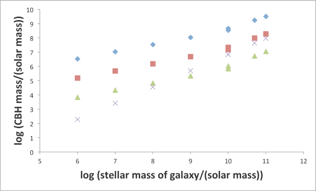
Figure 1:

References

- [1] Planck Collaboration, “Planck 2015 results. XIII. Cosmological parameters,” arXiv:1502.01589
- [2] Siemiginowska, A., et al, “The 300 kpc long X-ray jet in PKS 1127-145, z=1.18 quasar: Constraining X-ray emission models,” ApJ 657, 145, 2007
- [3] Bousso, R., “The holographic principle,” Rev. Mod. Phys. 74, 825, 2002
- [4] Misner, C., Thorne, K., & Wheeler, J., “Gravitation,” W. H. Freeman and Company, New York, 1973
- [5] Longair, S., “Galaxy Formation,” Springer-Verlag, Berlin, 1998; Jeans, J., "The Stability of a Spherical Nebula". Phil. Trans. Roy. Soc. 1902
- [6] Pearson, D., Batiste, M. & Batuski, D., “The Largest Gravitationally Bound Structures: The Corona Borealis Supercluster - Mass and Bound Extent,” MNRAS 441, 1601, 2014 [arXiv:1404.1308]
- [7] Crowther, P., “The R136 star cluster hosts several stars whose individual masses greatly exceed the accepted 150 Msun stellar mass limit,” [arXiv:1007.3284]
- [8] Massey, P. & Meyer, R., ”Stellar masses,” pg. 1, Encyclopedia of Astronomy and Astrophysics, 2001
- [9] Kroupa, P., “On the variation of the initial mass function,” MNRAS 322, 231, 2001 [arXi:astro-ph/0009005]
- [10] de Carvalho, J. & Macedo, P., “The structure formation in a quasi-static approximation,” Dark and Visible Matter in Galaxies. ASP Conf. Ser. 117, 310, 1997; Persic, M. & Salucci, P., eds.
- [11] Gnedin, O, and Ostriker, J, “Destruction of the Galactic Globular Cluster System,” ApJ 474, 223, 1997
- [12] Naoz, S., et al, “The First Stars in The Universe,” MNRAS Lett. 373:L98, 2006
- [13] Markevitch, M., et al, “Direct constraints on the dark matter self-interaction cross-section from the merging galaxy cluster 1E0657-56,” ApJ 606, 819, 2004
- [14] Wesson, P., “Clue to the unification of gravitation and particle physics,” Phys. Rev. D23, 1730, 1981
- [15] Forbes, D. & Kroupa, P., “What is a galaxy? Cast your vote here…,” arXiv:1101.3309
- [16] Shu, F. , “The Physical Universe - An Introduction to Astronomy,” University Science Books, 1982
- [17] Binney, J. & Tremaine, S., “Galactic Dynamics,” Princeton University Press, 1987
- [18] Bhattacharya, D., “Stellar Systems: two-body relaxation,” PH217: Aug-Dec 2003, http://meghnad.iucaa.ernet.in/~dipankar/ph217/relax.pdf
- [19] Pato, M., & Iocco, F., “The dark matter profile of the Milky Way: a non-parametric reconstruction,” [arxiv:1504.03317]
- [20] Marleau, F., Clancy, D. and Bianconi, M. “The Ubiquity of Supermassive Black Holes in the Hubble Sequence,” MNRAS 435, 3085, 2013 [arXiv:1212.0980]
- [21] Marleau, F. et al, “Infrared Signature of Active Massive Black Holes in Nearby Dwarf Galaxies,” arXiv:1411.3844,
- [22] Kafle, P., et al, “On the Shoulders of Giants: Properties of the Stellar Halo and the Milky Way Mass Distribution,” arXiv:1408.1787
- [23] Peñarrubia, J, et al, “A dynamical model of the local cosmic expansion,” arXiv:1405.0306
- [24] Ghez, A., et al, “Measuring Distance and Properties of the Milky Way’s Central Supermassive Black Hole with Stellar Orbits,” arXiv:0808.2870
- [25] Merrifield, M., Forbes, D. and Terlevich, A., “The black holes mass - galaxy age relation,” astro-ph/0002350
- [26] Bluck, A., et al, “Why do galaxies stop forming stars? I. The passive fraction - black hole mass relation for central galaxies” arXiv:1412.3862
- [27] Wu, X. et al., “An ultra-luminous quasar with a twelve-billion-solar-mass black hole at redshift 6.30,” Nature 518, 512, 2015 [arXiv:1502.0418]
- [28] Adler, R. & Overduin, J. “The Nearly Flat Universe,” Gen. Rel. Grav. 37, 1491, 2005 [gr-qc/0501061]