Wyner-Ziv Coding in the Real Field Based on BCH-DFT Codes

Abstract

We show how real-number codes can be used to compress correlated sources and establish a new framework for distributed lossy source coding, in which we quantize compressed sources instead of compressing quantized sources. This change in the order of binning and quantization blocks makes it possible to model correlation between continuous-valued sources more realistically and compensate for the quantization error when the sources are completely correlated. We focus on the asymmetric case, i.e., lossy source coding with side information at the decoder, also known as Wyner-Ziv coding. The encoding and decoding procedures are described in detail for discrete Fourier transform (DFT) codes, both for syndrome- and parity-based approaches. We also extend the parity-based approach to the case where the transmission channel is noisy and perform distributed joint source-channel coding in this context. The proposed system is well suited for low-delay communications. Furthermore, the mean-squared reconstruction error (MSE) is shown to be less than or close to the quantization error level, the ideal case in coding based on binary codes.

I Introduction

The distributed source coding (DSC) studies compression of statistically dependent sources which do not communicate with each other [1]. The Wyner-Ziv coding problem [2], a special case of lossy DSC, considers lossy data compression with side information at the decoder. The current approach to the DSC of continuous-valued sources is to first convert them to discrete-valued sources and then apply lossless (Slepian-Wolf) coder [3, 4, 5]. Similarly, a practical Wyner-Ziv encoder consists of a quantizer and Slepian-Wolf encoder. There are, hence, quantization and binning losses for the source coder. Despite this, rate-distortion theory promises that block codes of sufficiently large length are asymptotically optimal, and they can be seen as vector quantizers followed by fixed-length coders [6]. Therefore, practical Slepian-Wolf coders have been realized using different binary channel codes, e.g., LDPC and turbo codes [7, 8, 9]. These codes, however, are out of the question if low delay is imposed on the system as they may introduce excessive delay when the desired probability of error is very low.

In this paper, we establish a new framework for the Wyner-Ziv coding and distributed lossy source coding, in general. We propose to first compress the continuous-valued sources and then quantize them, as opposed to the conventional approach. The new framework is compared against the existing one in Fig. 1. It introduces the use of real-number codes (see, e.g., [10, 11, 12, 13, 14]), to represent correlated sources with fewer samples, in the real field.

To do compression, we generate syndrome or parity samples of the input sequence using a real-number channel code [10], similar to what is done to compress a binary sequence of data using binary channel codes. Then, we quantize these syndrome or parity samples and transmit them. There are still coding (binning) and quantization losses; however, since coding is performed before quantization, error correction is in the real field, and the quantization error can be corrected when two sources are completely correlated over a block of code. A second and more important advantage of this approach is the fact that the correlation channel model can be more realistic, as it captures dependency between continuous-valued sources rather than quantized sources. In the conventional approach, it is implicitly assumed that quantization of correlated signals results in correlated sequences in the binary domain; this may not necessarily be precise due to the nonlinearity of the quantization operation. To avoid any loss due to the inaccuracy of correlation model, we exploit the correlation between the continuous-valued sources before quantization.

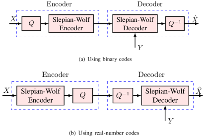
Figure 1: The Wyner-Ziv coding based on binary and real-number codes. Both schemes can be simply extended to distributed source coding.

The new approach is also capable of alleviating the quantization error. This is possible because coding precedes quantization. Specifically, we use the Bose-Chaudhuri-Hocquenghem (BCH) DFT codes for compression [10, 15, 16, 17, 18, 19]. Owing to DFT codes, the loss due to quantization can be decreased by a factor of $\frac{k}{n}$ for an $(n,k)$ code [20, 21, 19]. Additionally, reconstruction loss becomes zero if the two sources are perfectly correlated over one codeword. This is achieved in view of modeling the correlation between the two sources in the continuous domain. DFT codes also can exploit the temporal correlation typically found in many sources.

Finally, the proposed scheme is more suitable for low-delay communications since, even by using short DFT codes, a reconstruction error less than the quantization error is attainable. Moreover, as another contribution of this paper, we use a single DFT code both to compress and protect sources against channel variations. This extends the Wyner-Ziv coding to the case when errors occur during transmission and proposes joint source-channel coding (JSCC) with side information at the decoder, within the realm of real-number codes. This scheme directly maps short source blocks into channel blocks, and thus it is well suited to low-delay coding. While the MSE performance of distributed JSCC systems with binary codes is limited to the quantization error level, the proposed scheme breaks through this limit.

The paper is organized as follows. In Section II, we motivate the new framework for lossy DSC. In Section III, we study the encoding and decoding of DFT codes, and we adapt the subspace error localization to the Slepian-Wolf coder. Then in Section IV, we present the encoder and decoder for the Wyner-Ziv coding based on DFT codes, both for the syndrome and parity approaches. The system is extended to the noisy channel case in Section V. Section VI presents the simulation results. Section VII provides our concluding remarks.

For notation, we use upper-case and boldface lower-case letters for vectors, boldface upper-case letters for matrices, $(.)^{T}$ for transpose, $(.)^{H}$ for conjugate transpose, $(.)^{\ast}$ for conjugate, and $\mathop{\mathrm{tr}}(.)$ for the trace. The dimensions of matrices are indicated by one and two subscripts, when required.

II Real-Number Codes for DSC

II-A Motivations

Similar to error correction in finite fields, the basic idea of error correcting codes in the real field is to insert redundancy to a message vector to convert it to a longer vector, called the codeword. Nevertheless, the insertion of redundancy is done in the real field, i.e., before quantization and entropy coding [10, 11]. One main advantage of soft redundancy (real field codes) over hard redundancy (binary field codes) is that by using soft redundancy one can go beyond the quantization error level and thus reconstruct continuous-valued signals more accurately.

We introduce the use of real-number codes in lossy compression of correlated signals. The proposed system is depicted in Fig. 1. Although it consists of the same blocks as the existing Wyner-Ziv coding scheme [3, 4], the order of these blocks is changed here. Therefore binning is performed before quantization; we use DFT codes for this purpose [10, 16]. This change in the order of binning and quantization blocks brings some advantages to lossy DSC, as described in the following:

II-A1 Realistic correlation model

In the existing framework for lossy DSC, correlation between two sources is modeled after quantization, i.e., in the binary domain. More precisely, correlation between quantized sources is usually modeled as a binary symmetric channel (BSC), mostly with known crossover probability [5, 3, 4, 9]. Admittedly though, due to nonlinearity of the quantization operation, correlation between the quantized signals is not known accurately even if it is known in the continuous domain. This motivates us to investigate a method that exploits correlation between continuous-valued sources to perform DSC.

II-A2 Alleviating the quantization error

In lossy data compression with side information at the decoder, soft redundancy, added by DFT codes, can be used to correct both quantization errors and (correlation) channel errors. Thus, the loss due to quantization can be recovered, at least partly if not wholly. In fact, if the two sources are exactly the same over a codeword, the quantization error can be compensated for. That is, perfect reconstruction is attainable over the corresponding samples. The loss due to the quantization error is decreased by a factor of code rate even if correlation is not perfect, i.e., when (correlation) channel errors exist. This is because DFT codes are tight frames; hence, they minimize the MSE [20, 21, 19, 22].

II-A3 Low-delay communications

If communication is subject to low-delay constraints, we cannot use turbo or LDPC codes, as their performance is not satisfactory for short code length. low-delay coding has recently drawn a lot of attention; it is done by mapping short source blocks into channel blocks [23, 24]. Whether low-delay requirement exists or not depends on the specific applications. However, even in the applications that low-delay transmission is not imperative, it is sometimes useful to consider low-dimensional systems for their low computational complexity.

II-B Correlation Channel Model

Accurate modeling of the correlation between the sources plays a crucial role in the efficiency of the DSC systems. Most of the previous works assume that the correlation between continuous-valued sources can be modeled by an i.i.d. BSC in the binary field. This is not, however, exact because of the nonlinearity of quantization operation. Besides, independent errors in the sample domain are not translated to independent errors in the bit domain [25]. These issues can be avoided if we exploit the correlation between the continuous-valued sources before quantization.

The correlation between the analog sources $X$ and $Y$, in general, can be defined by

$$Y =X+E,$$ (1)

where $E$ is a real-valued random variable. Particularly, the above model represents some well-known models motivated in video coding and sensor networks. Let

$$E \sim\begin{cases}{\cal N}(0,\sigma_{e}^{2})\qquad\quad\quad\quad\text{ w.p. }\quad q_{1},\\ {\cal N}(0,\sigma_{e}^{2}+\sigma_{i}^{2})\quad\quad\,\,\,\,\,\text{ w.p. }\quad q_{2},\\ 0\qquad\quad\quad\quad\qquad\quad\;\,\text{ w.p. }\quad 1-q_{1}-q_{2},\\ \end{cases}$$ (2)

in which $\sigma_{i}^{2}\gg\sigma_{e}^{2}$ and $q_{1}+q_{2}\leq 1$. Then, for $q_{1}=1$ or $q_{2}=1$ the Gaussian correlation is obtained, which is broadly used in the sensor networks literature. Further, for $q_{1}+q_{2}=1$ the Gaussian-Bernoulli-Gaussian (GBG) and for $q_{1}+q_{2}<1$, $q_{1}q_{2}=0$ the Gaussian-Erasure (GE) models are realized. The latter two models are more suitable for video applications [26].

III BCH-DFT CODES: Construction and Decoding

In this section, we study a class of real-number codes that are employed for binning throughout this paper, investigate some properties of their syndrome, and adapt their decoding algorithm to the Slepian-Wolf coding. These codes are a family of Bose-Chaudhuri-Hocquenghem (BCH) codes in the real field whose parity-check matrix $\bm{H}$ and Generator matrix $\bm{G}$ are defined based on the DFT matrix; they are, thus, known as BCH-DFT codes, or simply DFT codes.

BCH-DFT codes[10] are linear block codes over the real or complex fields. Similar to other BCH codes, the spectrum of any codeword is zero in a block of $d\triangleq n-k$ cyclically adjacent components, where $d+1$ is the designed distance of that code [15]. The error correction capability of the code is, hence, given by $t=\lfloor\frac{d}{2}\rfloor$. In this paper, we only consider real BCH-DFT codes, i.e., the BCH-DFT codes whose generator matrix has real entries only.

III-A Encoding

An $(n,k)$ real BCH-DFT code is defined by its generator and parity-check matrices. The generator matrix is given by

$$\bm{G}=\sqrt{\frac{n}{k}}\bm{W}_{n}^{H}\bm{\Sigma}\bm{W}_{k},$$ (3)

in which $\bm{W}_{k}$ and $\bm{W}_{n}^{H}$ respectively are the DFT and IDFT matrices of size $k$ and $n$, and $\Sigma$ is an $n\times k$ matrix defined as

$$\bm{\Sigma}=\left(\begin{array}[]{ccccccc}\bm{I}_{\alpha}&\bm{0}\\ \bm{0}&\bm{0}\\ \bm{0}&\bm{I}_{\beta}\\ \end{array}\right),$$ (7)

where $\alpha=\lceil\frac{n}{2}\rceil-\lfloor\frac{n-k}{2}\rfloor$, $\beta=k-\alpha$, and the sizes of zero blocks are such that $\Sigma$ is an $n\times k$ matrix [27, 16, 18, 17]. Then, for any $\bm{u}$, this enforces the spectrum of the codeword

$$\bm{c}=\bm{G}\bm{u},$$ (8)

to have $n-k$ consecutive zeros, which is required for any BCH code [15]. The parity-check matrix $\bm{H}$, on the other hand, is constructed by using the $n-k$ columns of $\bm{W}_{n}^{H}$ corresponding to the $n-k$ zero rows of $\bm{\Sigma}$. Therefore, by virtue of the unitary property of $\bm{W}_{n}^{H}$, $\bm{H}$ is the null space of $\bm{G}$, i.e.,

$$\bm{HG}=\bm{0}.$$ (9)

In the rest of this paper, we use the term DFT code in lieu of real BCH-DFT code.

III-B Decoding

Before introducing the decoding algorithm, we define some notation and basic concepts. Let $\bm{r}=\bm{c}+\bm{e}$ be the received vector (a noisy version of $\bm{c}$), where $\bm{c}$ is a codeword generated by (8). Suppose that $\bm{e}$ is an error vector with $\nu$ nonzero elements at positions $i_{1},\ldots,i_{\nu}$; the magnitude of error at position $i_{p}$ is $e_{i_{p}}$. Then, we can compute

$$\mbox{\boldmath$\bm{s}=\bm{Hr}=\bm{H}(\bm{c}+\bm{e})=\bm{He}$},$$ (10)

where $\bm{s}=[s_{1},\,s_{2},\ldots,s_{d}]^{T}$ is a complex vector with

$$s_{m}=\frac{1}{\sqrt{n}}\sum_{p=1}^{\nu}e_{i_{p}}X_{p}^{\alpha-1+m},\qquad m=1,\ldots,d$$ (11)

in which $\alpha=\lceil\frac{k+1}{2}\rceil$ as defined in (7), $X_{p}=e^{\frac{-j2\pi i_{p}}{n}}$, and $p=1,\ldots,\nu.$ Next, we define the syndrome matrix

$$\bm{S}_{m} =\left[\begin{array}[]{cccc}s_{1}&s_{2}&\ldots&s_{d-m+1}\\ s_{2}&s_{3}&\ldots&s_{d-m+2}\\ \vdots&\vdots&\ddots&\vdots\\ s_{m}&s_{m+1}&\ldots&s_{d}\\ \end{array}\right],$$ (16)

for $\nu+1\leq m\leq d-\nu+1$ [16]. Also, we define the covariance matrix as

$$\bm{R}=\bm{S}_{m}\bm{S}_{m}^{H}.$$ (17)

For decoding, we use the extension of the well-known Peterson-Gorenstein-Zierler (PGZ) algorithm to the real field [15]. This algorithm, aimed at detecting, localizing, and calculating the errors, works based on the syndrome of error. We summarize the main steps of this algorithm, adapted for a DFT code of length $n$, in the following.

• Error detection: Determine the number of errors $\nu$ by constructing a syndrome matrix and finding its rank.

• Error localization: Find the coefficients $\Lambda_{1},\ldots,\Lambda_{\nu}$ of the error-locating polynomial $\Lambda(x)=\prod_{\begin{subarray}{c}i=1\end{subarray}}^{\nu}(1-xX_{i})$ whose roots $X_{1}^{-1},\ldots,X_{\nu}^{-1}$ are used to determine error locations; the errors are then in the locations $i_{1},\ldots,i_{\nu}$ such that $X_{1}=\omega^{i_{1}},\ldots,X_{\nu}=\omega^{i_{\nu}}$ and $\omega=e^{-j\frac{2\pi}{n}}$.

• Error calculation: Finally, calculate the error magnitudes by solving a set of linear equations whose constants coefficients are powers of $X_{i}$.

In practice however, the received vector is distorted because of quantization. Let $\bm{\hat{c}}$ and $\bm{q}$ denote the quantized codeword and quantization noise so that $\bm{\hat{c}}=\bm{c}+\bm{q}$. Therefore, $\bm{r}=\bm{\hat{c}}+\bm{e}$ and its syndrome is no longer equal to the syndrome of error because

$$\bm{Hr}=\bm{H}(\bm{c}+\bm{q}+\bm{e})=\bm{s}_{q}+\bm{s}=\tilde{\bm{s}},$$ (18)

where $\bm{s}_{q}\equiv\bm{Hq}$ and $\bm{q}=[q_{1},\,q_{2},\ldots,q_{n}]^{T}$ is the quantization error. The distorted syndrome samples can be written as

$$\tilde{s}_{m}=\frac{1}{\sqrt{n}}\sum_{p=1}^{\nu}e_{i_{p}}X_{p}^{\alpha-1+m}+\frac{1}{\sqrt{n}}\sum_{p^{\prime}=1}^{n}q_{i_{p^{\prime}}}X_{p^{\prime}}^{p^{\prime}-1}.$$ (19)

The distorted syndrome matrix $\tilde{\bm{S}}_{m}$ and the corresponding covariance matrix $\tilde{\bm{R}}=\tilde{\bm{S}}_{m}\tilde{\bm{S}}_{m}^{H}$ are defined similar to (16) and (17) but for the distorted syndrome samples.

While the exact value of the error is determined neglecting quantization, the decoding becomes an estimation problem in the presence of quantization. Then, it is imperative to modify the PGZ algorithm to decode the errors reliably [15, 16, 18, 17, 19]. In the remainder of this section, we discuss this problem and also improve the error detection and localization, by introducing a slightly different version of the existing methods.

III-B1 Error detection

For a given DFT code, we first fix an empirical threshold $\theta$ based on eigendecomposition of $\tilde{\bm{R}}$ when the codewords are error-free, i.e., when only the quantization error exist. This threshold is on the magnitude of eigenvalues, rather than the determinant of $\tilde{\bm{R}}$. Let $\lambda_{\mathrm{max}}$ denote the largest eigenvalue of $\tilde{\bm{R}}$ for $m=t+1$. We find $\theta$ such that, for a desired probability of correct detection $p_{d}$,

$$\mathrm{Pr}(\lambda_{\mathrm{max}}<\theta)\geq p_{d}.$$ (20)

In practice, when errors can occur, we estimate the number of errors by the number of eigenvalues of $\tilde{\bm{R}}$ greater than $\theta$. This one step estimation is better than the original estimation in the PGZ algorithm [15, 18], where the last row and column of $\bm{S}_{t}$ are removed until coming up with a non-singular matrix. The improvement comes from incorporating all syndrome samples, rather than some of them, for decision making.

III-B2 Error localization

The Subspace or coding-theoretic error localizations [16] can be used to find the coefficients $\Lambda_{1},\ldots,\Lambda_{\nu}$ of the error-locating polynomial. The subspace approach is, however, more general than the coding-theoretic approach in the sense that it can use up to $t+1-\nu$ degrees of freedom to localize $\nu$ errors, compared to just one degree of freedom in the coding-theoretic approach. Hence, it improves the error localization in the presence of the quantization noise. We apply the subspace error localization both to the syndrome- and parity-based DSC (see Section IV), similar to that in channel coding [16]. To this end, we eigen-decompose the covariance matrix $\tilde{\bm{R}}=\tilde{\bm{S}}_{m}\tilde{\bm{S}}_{m}^{H}$ for $m=t+1.$ It results in two orthogonal subspaces, the error and noise subspaces. There are $m-\nu$ vectors in the noise subspace; we use them to localize errors using the MUSIC algorithm [16, 28]. However, one should note that the way we compute the syndrome in DSC is different from that in channel coding which was presented in (10) and (18); this will be elaborated in Section IV.

III-B3 Error calculation

This last step is rather simple. Let $\bm{H}_{e}$ be the matrix consisting of the columns of $H$ corresponding to error indices. The errors magnitude $\bm{e}=\left[e_{i_{1}},\,e_{i_{2}},\ldots,e_{i_{\nu}}\right]^{T}$ can be determined by solving

$$\bm{H}_{e}\bm{e}=\tilde{\bm{s}},$$ (21)

in a least squares sense, for example. This completes the error correction algorithm by calculating the error vector.

III-C Performance Compared to Binary Codes

DFT codes by construction are capable of decreasing the quantization error. When there is no error, an $(n,k)$ DFT code brings down the MSE below the quantization error level with a factor of $R_{c}=k/n$ [21, 20]. This is also shown to be valid for channel errors, as long as channel can be modeled as an additive noise. To appreciate this, one can consider the generator matrix of a DFT code as analysis frame operator of a tight frame [21]; it is known that frames are resilient to any additive noise, and tight frames reduce the MSE $k/n$ times [29]. Hence, DFT codes can result in a MSE even less than the quantization error level whereas the MSE in a binary code is obviously lower-bounded by the quantization error level.

IV Wyner-Ziv Coding Using DFT Codes

In this section, we use DFT codes to do Wyner-Ziv coding in the real field. This is accomplished by using DFT codes for binning and transmitting compressed signal, in the form of syndrome or parity samples, in a digital communication system. Let $x$ be a sequence of real random variables $x_{1}x_{2}\ldots x_{n}$, and $y$ be a noisy version of $x$ such that $y_{i}=x_{i}+e_{i}$, where $e_{i}$ is continuous, i.i.d., and independent of $x_{i}$, as described in (2). The lower-case letters $x$, $y$, and $e$, respectively, are used to show the realization of the random variables $X$, $Y$, and $E$. Since $\bm{e}$ is continuous, this model precisely captures any variation of $\bm{x}$, so it can model correlation between $x$ and $y$ accurately. This correlation model is important, for example, in video coders that exploit Wyner-Ziv concepts, e.g., when the decoder builds side information via extrapolation of previously decoded frames or interpolation of key frames [26]. In this paper, we use the GE model with $q_{2}=0$ in (2) where $\bm{e}$ is a sparse vector inserting up to $t$ errors in each codeword.

IV-A Syndrome Approach

IV-A1 Encoding

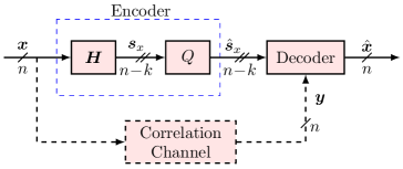
Figure 2: The Wyner-Ziv coding using DFT codes: Syndrome approach.

Given $H$, to compress an arbitrary sequence of data samples, we multiply it with $H$ to find the corresponding syndrome samples $s$_x$=Hx$. The syndrome is then quantized ($\hat{s}$_x$\;=\;$$s$_x$\;+\;\mbox{\boldmath$q$}$) and transmitted over a noiseless digital communication system, as shown in Fig. 2. Note that $s$_x, $\hat{s}$_x are both complex vectors of length $n-k$. Thus, it seems that to transmit each sample we need to send two real numbers, one for the real part and one for the imaginary part, which halves the compression ratio. However, we observe that the syndrome of a DFT code is symmetric, as stated below.

Lemma 1.

The syndrome of an $(n,k)$ DFT code satisfies

$$s_{m}=\left\{\begin{array}[]{l l}s_{d-m+1}^{\ast},&\quad\text{if $k$ is odd,}\\ s_{d-m}^{\ast},&\quad\text{if $k$ is even,}\end{array}\right.$$ (24)

for $m=1,\ldots,d$ and $d\triangleq n-k$.

Proof.

See Appendix VIII-A. ∎

The above lemma implies that, for any $d$, it suffices to know the first $\lceil\frac{d}{2}\rceil$ syndrome samples. We know that syndromes are complex numbers in general; however, from $s_{d-m+1}=s_{m}^{\ast}$ it is clear that if $d$ is an odd number, $s_{m}$ is real for $m=\lceil\frac{d}{2}\rceil$. Therefore, for an $(n,k)$ code with odd $k$, transmitting $n-k$ real numbers suffices. This results in a compression ratio of $\frac{n}{n-k}$ for the Slepian-Wolf encoder. Yet, one can check that for even $k$, we have to transmit $n-k+1$ real samples, which incurs a slight loss in compression. It is however negligible for large $n$.

IV-A2 Decoding

The decoder estimates the input sequence from the received syndrome and side information $\bm{y}$. To this end, it needs to evaluate the syndrome of (correlation) channel errors. This can be simply done by subtracting the received syndrome from the syndrome of the side information. Then, neglecting the quantization error, we obtain,

$$\mbox{\mbox{\boldmath$s$}${}_{e}$$\;=\;$\mbox{\boldmath$s$}${}_{y}$$\;-\;$\mbox{\boldmath$s$}${}_{x}$},$$ (25)

and $s$_e can be used to precisely estimate the error vector, as described in Section III-B. In practice, however, the decoder knows $\hat{s}$_x$\;=\;$$s$_x$\;+\;\mbox{\boldmath$q$}$ rather than $s_{x}$. Therefore, only a distorted syndrome of error is available, i.e.,

$$\mbox{\mbox{\boldmath$\tilde{s}$}${}_{e}$$\;=\;$\mbox{\boldmath$s$}${}_{y}$$\;-\;$\mbox{\boldmath$\hat{s}$}${}_{x}$$\;=\;$\mbox{\boldmath$s$}${}_{e}$$\;-\;$ \mbox{\boldmath$q$}}.$$ (26)

Hence, using the PGZ algorithm, error correction is accomplished based on (26). Note that, having computed the syndrome of error, decoding algorithm in a DSC using DFT codes is exactly the same as that in the channel coding problem. This is different from DSC techniques in the binary field which usually require a slight modification in the corresponding channel coding algorithm to be customized for DSC.

IV-B Parity Approach

The syndrome-based Wyner-Ziv coding is straightforward, but it is not clear how we can use it for noisy transmission. In the sequel, we explore an alternative approached, namely parity-based approach, to the Wyner-Ziv coding.

IV-B1 Encoding

To compress $\bm{x}$, the encoder generates the corresponding parity sequence $\bm{p}$ with $n-k$ samples. The parity is then quantized and transmitted, as shown in Fig. 3, instead of transmitting the input data. To this end, we need to find a systematic generator matrix $\bm{G}_{\mathrm{sys}}$, as $\bm{G}$ in (3) is not in the systematic form.

A first approach is to find $\bm{H}_{\mathrm{sys}}$ and build $\bm{G}_{\mathrm{sys}}$ based on that [30]. Another, simpler, way is to obtain a systematic generator matrix directly from $\bm{G}$. Let $\bm{G}_{k}$ be a square matrix of size $k$ composed of arbitrary rows of $\bm{G}$. We see that $\bm{G}_{k}$ is invertible because using (3) any $k\times k$ submatrix of $\bm{G}$ can be represented as product of a Vandermonde matrix and the DFT matrix $\bm{W}_{k}$. This is also proven using a different approach in [21], where it is shown that any subframe of $\bm{G}$ is a frame, and its rank is equal to $k$. Hence, a systematic generator matrix is given by

$$\bm{G}_{\mathrm{sys}}=\bm{G}\bm{G}_{k}^{-1}.$$ (27)

Besides, from $\bm{H}\bm{G}=\bm{0}$, it is clear that

$$\bm{H}\bm{G}_{\mathrm{sys}}=\bm{0}.$$ (28)

Therefore, we do not need to calculate $\bm{H}_{\mathrm{sys}}$, and the same parity-check matrix $\bm{H}$ can be used for decoding in the parity approach. It is also obvious that $\bm{G}_{\mathrm{sys}}$ is a real matrix. The question that remains to be answered is whether $\bm{G}_{\mathrm{sys}}$ corresponds to a BCH code. To generate a BCH code, $\bm{G}_{\mathrm{sys}}$ must have $n-k$ consecutive zeros in the transform domain. The Fourier transform of this matrix $\bm{W}_{n}\bm{G}_{\mathrm{sys}}=(\bm{W}_{n}\bm{G})\bm{G}_{1}^{-1}$ satisfies the required condition because $\bm{W}_{n}\bm{G}$, the Fourier transform of original matrix, satisfies that.

Figure 3: The Wyner-Ziv coding using DFT codes: Parity approach.

It should be emphasized that one can arbitrarily choose the rows of $\bm{G}_{k}$ in (27); this results in $\binom{n}{k}$ systematic generator matrix for an $(n,k)$ DFT code. Although any of those systematic codes can be used for encoding, the dynamic range of the generated parity samples depends on their relative position of the chosen rows [27]. In [31, Theorem 7], we have proved that when using these systematic frames for error correction, the mean-squared reconstruction error is minimized when the systematic rows are chosen as evenly spaced as possible. In the extreme scenario, where the systematic rows are equally spaced, the systematic frame is also tight. This is realized only when $n$ is an integer multiple of $k$. Such a frame lends itself well to minimize reconstruction error [20, 32, 21, 22].

Finally, seeing that parity samples are real numbers, using an $(n,k)$ DFT code, a compression ratio of $\frac{k}{n-k}$ is achieved. Obviously, a compression ratio of $\frac{n}{n-k}$ is achievable if we use a $(2n-k,n)$ DFT code.

IV-B2 Decoding

A parity decoder estimates the input sequence from the received parity and side information $\bm{y}$. Similar to the syndrome approach, at the decoder, we need to find the syndrome of (correlation) channel errors. To do so, we append the parity to the side information and form a vector of length $n$ whose syndrome, neglecting quantization, is equal to the syndrome of error. That is,

$$\bm{z}=\left[\begin{array}[]{cc}\bm{y}\\ \bm{p}\\ \end{array}\right]=\left[\begin{array}[]{cc}\bm{x}\\ \bm{p}\end{array}\right]+\left[\begin{array}[]{cc}\bm{e}\\ \bm{0}\end{array}\right]=\bm{G}_{\mathrm{sys}}\bm{x}+\bm{e}^{\prime},$$ (35)

and $\bm{e}^{\prime}=[\bm{e}\;|\;\bm{0}]^{T}$. Hence,

$$\bm{s}_{z}=\bm{s}_{e^{\prime}}.$$ (36)

Similarly, when quantization is involved ($\bm{\hat{p}}=\bm{p}+\bm{q}$), we get

$$\bm{\tilde{z}}=\left[\begin{array}[]{cc}\bm{y}\\ \bm{\hat{p}}\\ \end{array}\right]=\bm{z}+\left[\begin{array}[]{cc}\bm{0}\\ \bm{q}\end{array}\right]=\bm{G}_{\mathrm{sys}}\bm{x}+\bm{e}^{\prime}+\bm{q}^{\prime},$$ (41)

and

$$\bm{s}_{\tilde{z}}=\bm{s}_{e^{\prime}}+\bm{s}_{q^{\prime}},$$ (42)

where, $\bm{q}^{\prime}=[\bm{q}\;|\;\bm{0}]^{T}$, and $\bm{s}_{q^{\prime}}\equiv\bm{Hq}^{\prime}$. Therefore, we obtain a distorted version of error syndrome. In both cases, the rest of the algorithm, which is based on the syndrome of error, is similar to that in the channel coding problem using DFT codes, as explained in Section III-B2.

Error localization algorithm for the parity-based DSC [30] can be further improved using the fact that parity samples are error-free. As parity samples are transmitted over a noiseless channel, the error locations, in the codewords, are restricted to the systematic samples. Therefore, we can exclude the set of roots corresponding to the location of the parity samples. We call this adapted error localization. Furthermore, it makes sense to use a code with evenly-spaced parity samples so as to optimize the location of error-free and error-prone samples in the codewords. Such a code maximizes the distance between the error-prone roots of the code; hence, it helps decrease the probability of incorrect decision.

IV-C Comparison Between the Two Approaches

IV-C1 Rate

As it was shown earlier, using an $(n,k)$ code the compression ratio in the syndrome and parity approaches, respectively, is $\frac{n}{n-k}$ and $\frac{k}{n-k}$. Hence, for a given code, the parity approach is $\frac{k}{n}=R_{c}<1$ times less efficient than the syndrome approach. Conversely, we can find two different codes that result in same compression ratio, say $\frac{n}{n-k}$. We mentioned that in the parity approach, a $(2n-k,n)$ code can be used for this matter, whereas an $(n,k)$ DFT code gives the desired compression ratio in the syndrome approach. Thus, for a given compression ratio the syndrome approach implies a code with smaller rate compared to the code required in the parity approach.

IV-C2 Performance

From frame theory, we know that DFT frames are tight, and an $(n,k)$ tight frame reduces the quantization error with a factor of $R_{c}=\frac{k}{n}$ [29, 21, 20]. This result is extended to errors, given that channel can be modeled by an additive noise [19]. The MSE performance of systematic DFT frames also linearly depends on the code rate, though they are not necessarily tight [27, 31]. Therefore, for codes with the same error correction capability, the lower the code rate the better the error correction performance. This implies a better performance for syndrome-based DSC. Further, a $(2n-k,n)$ code has $n-k$ roots more than an $(n,k)$ code on the unit circle; hence, the roots are closer to each other and the probability of incorrect localization of errors increases.

Additionally, from rate-distortion theory we know that the rate required to transmit a Gaussian source logarithmically increases with the source variance [33]. Thus, in a system that uses a real-number code for encoding, since coding is performed before quantization, the variance of transmitted sequence depends on the behavior of the encoding matrix. In the syndrome-based DSC we transmit $\bm{s}=\bm{H}\bm{x}$. One can check that $\sigma_{\bm{s}}=\sigma_{\bm{x}}$ [31]. Unlike that, in the parity-based DSC, the variance of the parity samples is larger than that of the inputs. More precisely, in an $(n,k)$ systematic DFT code, if $\bm{c}=\bm{G}_{\mathrm{sys}}\bm{x}$, then $\sigma^{2}_{\bm{c}}=\gamma\sigma^{2}_{\bm{x}}$ where $\gamma=\frac{1}{n}\mathop{\mathrm{tr}}\left(\bm{G}_{\mathrm{sys}}^{H}\bm{G}_{\mathrm{sys}}\right)\geq 1$ [27]. Since we can write $c=[\bm{x}\;|\;\bm{p}]^{T}$, we have

$$\sigma^{2}_{\bm{p}}=\frac{\gamma n-k}{n-k}\sigma^{2}_{\bm{x}}\geq\sigma^{2}_{\bm{x}}.$$ (43)

From [31, Theorem 7], we know that the smallest $\sigma_{\bm{p}}$ for a given DFT code is achieved when the parity samples, in the corresponding codewords, are located as “evenly” as possible.

Considering the above arguments, one may expect the syndrome-based approach to perform better than the parity-based one, for a given code or fixed compression ratio. This is verified numerically in Section VI. The parity-based DSC, however, has other advantages. For example, by puncturing some parity samples rate-adaptive DSC, in the real field, is realized. Besides, it can be easily extended to distributed joint source-channel coding, as explained in the following section.

V Distributed Joint Source and Channel Coding

The concept of lossy DSC and Wyner-Ziv coding using DFT codes was explained both for the syndrome and parity approaches in Section IV, where syndrome or parity samples are quantized and transmitted over a noiseless channel. This implies separate source and channel coding. Although simple, the separation theorem is based on several assumptions, such as the source and channel coders not being constrained in terms of complexity and delay, which do not hold in many situations. It breaks down, for example, for non-ergodic channels and real-time communication. In such cases, it makes sense to integrate the design of the source and channel coder systems, because joint source-channel coding (JSCC) can perform better given a fixed complexity and/or delay constraints. Likewise, distributed JSCC (DJSCC) has been shown to outperform separate distributed source and channel coding in some practical cases [34]. DJSCC has been addressed in [9, 34, 35, 36], using different binary codes.

In this section, we extent the parity-based Wyner-Ziv coding of analog sources to the case where errors in the transmission are allowed. Thus, we introduce distributed JSSC of analog correlated sources in the analog domain. To do this, we use a single DFT code both to compress $\bm{x}$ and protect it against channel variations; this gives rise to a new framework for DJSCC, in which quantization is performed after doing JSCC in the analog domain. This scheme directly maps short source blocks into channel blocks, and thus it is well suited to low-delay coding.

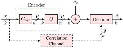
Figure 4: Joint source-channel coding (JSCC) with side information at the decoder based on DFT codes. Obviously, the scheme can be extended to distributed JSCC.

V-A Coding and Compression

To compress and protect $\bm{x}$, the encoder generates the parity sequence $\bm{p}$ of $n-k$ samples, with respect to a good systematic DFT code. The parity is then quantized and transmitted over a noisy channel, as shown in Fig. 4. To keep the dynamic range of parity samples as small as possible, we make use of optimal systematic DFT codes, proposed in [31]. This increases the efficiency of the system for a fixed number of quantization levels. Using an $(n,k)$ DFT code a total compression ration of $\frac{n}{n-k}$ is achieved. Obviously, if $n<2k$ compression is possible. However, since there is little redundancy the end-to-end distortion could be high. Conversely, a code with $n>2k$ expands input sequence by adding soft redundancy to protect it in a noisy channel.

V-B Decoding

Let $\tilde{\bm{p}}=\hat{\bm{p}}+\bm{e}_{c}$ be the received parity vector which is distorted by quantization error $\bm{q}$ ($\hat{\bm{p}}=\bm{p}+\bm{q}$) and channel error $\bm{e}_{c}$. Also, let $\bm{y}=\bm{x}+\bm{e}_{v}$ denote side information where $\bm{e}_{v}$ represents the error due to the “virtual” correlation channel. The objective of the decoder is to estimate the input sequence from the received parity and side information. Although we only need to determine $\bm{e}_{v}$, effectively it is required to find both $\bm{e}_{v}$ and $\bm{e}_{c}$. From an error correction point of view, this is equal to finding the error vector $\bm{e}=[\bm{e}_{v}\;\;\bm{e}_{c}]^{T}$ that affects the codeword $[\bm{x}\;\;\bm{p}]^{T}$. Hence, to find the syndrome of error at the decoder, we append the parity $\tilde{\bm{p}}$ to the side information $\bm{y}$ and form $\tilde{\bm{z}}$, a valid codeword perturbed by quantization and channel errors,

$$\tilde{\bm{z}}=\left[\begin{array}[]{cc}\bm{x}\\ \bm{p}\end{array}\right]+\left[\begin{array}[]{cc}\bm{e}_{v}\\ \bm{e}_{c}\end{array}\right]+\left[\begin{array}[]{cc}\bm{0}\\ \bm{q}\end{array}\right]=\bm{G}_{\mathrm{sys}}\bm{x}+\bm{e}+\bm{q}^{\prime}.$$ (50)

Multiplying both sides by $\bm{H}$, we obtain

$$\bm{s}_{\tilde{z}}=\bm{s}_{e}+\bm{s}_{q^{\prime}},$$ (51)

where $\bm{s}_{e}\equiv\bm{He}$ and $\bm{s}_{q^{\prime}}\equiv\bm{Hq}^{\prime}$. Again, we use the GE model with $q_{2}=0$ in (2) to generate $\bm{e}$. It should be emphasized that for $\bm{q}=\bm{0}$, error vector can be determined exactly, as long as the number of errors is not greater than $t$. In practice, quantization is also involved, and we obtain only a distorted version of error syndrome. Knowing the syndrome of error, we use the error detection and localization algorithm, explained in Section III-B, to find and correct error.

VI Simulation Results

We evaluate the performance of the proposed systems using a Gauss-Markov source with mean zero, variance one, and correlation coefficient 0.9; the effective range of the input sequences is thus $[-4,4]$. The sources are binned using a $(7,5)$ DFT code. The compressed vector, either syndrome or parity, is then quantized with a 6-bit uniform quantizer with step size $\Delta=0.125$ and transmitted over a noiseless communication media. The “virtual” correlation channel inserts $t$ errors, generated by $\mathcal{N}(0,\sigma_{e}^{2})$. The decoder detects, localizes, and decodes errors. We compare the MSE between transmitted and reconstructed codewords, to measurers end-to-end distortion. In all simulations, we use $10^{5}$ input blocks for each channel-error-to-quantization-noise ratio (CEQNR), defined as $\sigma_{e}^{2}/\sigma_{q}^{2}$ and $\sigma_{q}^{2}=\frac{\Delta^{2}}{12}$. We vary the CEQNR and plot the resulting MSE. The results are presented in Fig. 5 and compared against the quantization error level in the existing lossy DSC methods.

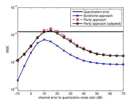
Figure 5: Reconstruction error in the syndrome and parity approaches, using a $(7,5)$ DFT code in Fig. 2, 3. For both schemes, the virtual correlation channel inserts one error at each input block.

It can be observed that, in the syndrome approach the MSE is lower than the quantization error level in all CEQNRs. Analogously, in the parity approach, the MSE is less than that level except for a small range of CEQNR; further, it slightly improves when we use the adapted parity approach. Note that in lossy DSC using binary codes, the MSE can be equal to the quantization error level only if the bit error rate (BER) for the Slepian-Wolf coder is zero. This ideal case is not necessarily attainable even if capacity-approaching codes are used [25]. The performance of our systems considerably improves when CEQNR is very high. The improvement is due to a better error localization, since the higher the CEQNR, the better the error localization, as shown in Fig. 6. At very low CEQNRs, although error localization is poor, the MSE is still very low. This is because, compared to the quantization error, the errors are so small that the algorithm mostly does not detect (and thus localize) any error. Instead, it may occasionally localize and correct quantization errors. Note that, even if no errors are localized and corrected, the MSE is still very small as the errors are negligible at very low CEQNRs. Additionally, recall that the MSE is always reduced with a factor of $R_{c}=\frac{k}{n}$, in an $(n,k)$ DFT code [20, 21, 19]. It should be added that, for error detection, we use the algorithm proposed in Section III-B1; for this purpose, we first find the threshold corresponding to $p_{d}=90\%$; it leads to $\theta=0.0014$. The corresponding plots are not included, for brevity; even so, similar plots are studied in the remainder of this section.

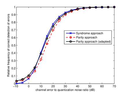
Figure 6: Relative frequency of correct localization of correlation channel error in the syndrome and parity approaches, using a $(7,5)$ DFT code. Since $\nu=t=\frac{n-k}{2}$, the coding theoretic and subspace error localizations give the same results; hence, we employ one of them in this set of plots. For the parity approach, we also plot the adapted error localization, introduced in Section IV-B2, as well.

In terms of compression, the efficiency of parity approach to the syndrome approach is $R_{c}=\frac{5}{7}$, as discussed earlier in Section IV-C. Despite this, the performance of the parity approach is not as good as that of the syndrome approach. One reason is that in this simulation $1/5$ of samples are corrupted in the parity approach while this figure is $1/7$ for the syndrome approach. More importantly, the dynamic range of the parity samples, generated by (27), could be much higher than that of the syndrome samples; this range depends on the position of the parity samples in the codewords. A wider range implies more quantization levels to achieve the same accuracy. For the $(7,5)$ code, in the best case we get $\sigma_{p}=2.17\sigma_{x}$ since $\gamma_{\min}=2.0645$ in (43). This is realized for a codeword pattern $\times\times\times-\times\times-$, where “$\times$’s” and “$-$’s” represent data and parity samples, respectively.

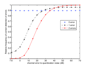
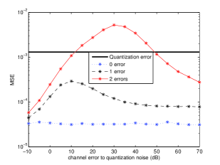
Figure 7: Performance evaluation of joint source-channel coding with side information at the decoder, proposed in Fig. 4, for $(10,5)$ DFT code. 7 Histogram of $\lambda_{\mathrm{max}}(\tilde{\bm{R}})$ for a quantized code. This is used to set a threshold for detection. 7 Probability of correct detection of errors. 7 Probability of correct localization of errors. 7 The end-to-end distortion (MSE).

Next, we evaluate the performance of the JSCC with side information at the decoder, illustrated in Fig. 4. By using a systematic $(10,5)$ DFT code, we generate, quantize, and transmit parity samples over a noisy channel. Note that, for this code the best systematic code [27] achieves the lower bound in (43); i.e., it results in $\sigma_{p}=\sigma_{x}$. The correlation channel and transmission channel altogether insert up to $t$ errors generated by $\mathcal{N}(0,\sigma_{e}^{2})$. Simulation results are plotted in Fig. 7. First, based on Fig. 7, the threshold $\theta=0.0065$ is fixed for $p_{d}=90\%$. Next, this is used to estimate $\nu$ in Fig. 7. The estimated number is subsequently used to find the location of errors, both for the PGZ and subspace methods, in Fig. 7. Then, the output of Fig. 7, for the subspace method, is fed to the last step to find the magnitude of errors and correct them. Finally, in Fig. 7, the MSE is compared against the quantization error level, the ideal case in the lossy source coding based on binary codes. To put our results in perspective, we also calculate the MSE assuming perfect error localization; it gives $0$, $6.5\times 10^{-5}$, and $1.8\times 10^{-4}$ respectively for 0, 1, and 2 errors, in every CEQNR. This implies that there is still room to improve the MSE performance of the proposed system, given a better solution for the error localization. It also shows the performance gap between this DFT code and binary codes in the ideal case.

It should be noted that capacity-approaching channel codes may introduce significant delay if one strives to approach the capacity of the channel with very a low probability of error. Therefore, those are out of the question for delay-sensitive systems. In that case, it would be best to use channel codes of low rate and focus on achieving a very low probability of error. The system we introduced is a low-delay system which works well with reasonably high-rate codes. Finally, by puncturing some parity samples, rate-adaptive schemes are realized for the proposed DJSCC and parity-based DSC. Rate-adaptive systems are popular in the transmission of non-ergodic data, like video [37].

VII Conclusions

We have introduced a new framework for the distributed lossy source coding, in general, and the Wyner-Ziv coding, in particular. The idea is to do binning before quantizing the continuous-valued signal, as opposed to the conventional approach where binning is done after quantization. By doing binning in the real field, the virtual correlation channel can be modeled more accurately and the quantization error can be compensated for when there is no error. In the new paradigm, Wyner-Ziv coding is realized by cascading a Slepian-Wolf encoder with a quantizer. We employ real BCH-DFT codes to do the Slepian-Wolf in the real field. At the decoder, by introducing both syndrome-based and parity-based systems, we adapt the PGZ decoding algorithm of channel coding to DSC. The extension of the parity-based Wyner-Ziv coding to joint source-channel coding with side information at the decoder is straightforward. This scheme directly maps short source blocks into channel blocks, and thus it is appropriate for low-delay coding. From simulation results, we conclude that our systems can improve the reconstruction error even using short codes, so they can become viable in real-world scenarios where low-delay communication is required.

We have also adapted the subspace error localization in this context and improved it for the parity-based scheme. This reasonably improves the error localization and leads to a better mean-squared reconstruction error. We should point out that, a more accurate algorithm for error localization is a key to further improve the reconstruction error. Particularly, error localization becomes more challenging when codeword length increases, as the roots of error locator polynomial, which are over the unit circle, get closer.

VIII Appendix

VIII-A Proof of Lemma 1

Proof.

The proof is straightforward; we show this for odd $k$ and leave the other case to the reader. Since $\alpha=\lceil\frac{k+1}{2}\rceil$ and $d=n-k$, using (11), for odd $k$ we can write

$$s_{d-m+1} =\frac{1}{\sqrt{n}}\sum_{p=1}^{\nu}e_{i_{p}}X_{p}^{\frac{k-1}{2}+n-k-m+1}$$

$$=\frac{1}{\sqrt{n}}\sum_{p=1}^{\nu}e_{i_{p}}X_{p}^{\frac{-k+1}{2}-m}=s_{m}^{\ast}.$$

Note that $X_{p}^{n}=1$, for any $p$. ∎

References

- [1] D. Slepian and J. K. Wolf, “Noiseless coding of correlated information sources,” IEEE Transactions on Information Theory, vol. IT-19, pp. 471–480, July 1973.
- [2] A. D. Wyner and J. Ziv, “The rate-distortion function for source coding with side information at the decoder,” IEEE Transactions on Information Theory, vol. 22, pp. 1–10, Jan. 1976.
- [3] B. Girod, A. M. Aaron, S. Rane, and D. Rebollo-Monedero, “Distributed video coding,” Proceedings of the IEEE, vol. 93, pp. 71–83, Jan. 2005.
- [4] Z. Xiong, A. D. Liveris, and S. Cheng, “Distributed source coding for sensor networks,” IEEE Signal Processing Magazine, vol. 21, pp. 80–94, Sept. 2004.
- [5] S. S. Pradhan and K. Ramchandran, “Distributed source coding using syndromes (DISCUS): Design and construction,” IEEE Transactions on Information Theory, vol. 49, pp. 626–643, March 2003.
- [6] P. L. Dragotti and M. Gastpar, Distributed Source Coding: Theory, Algorithms, and Applications. Academic Press, 2009.
- [7] A. D. Liveris, Z. Xiong, and C. N. Georghiades, “Compression of binary sources with side information at the decoder using LDPC codes,” IEEE Communications Letters, vol. 6, pp. 440–442, Oct. 2002.
- [8] J. Bajcsy and P. Mitran, “Coding for the Slepian-Wolf problem with turbo codes,” in Proc. IEEE Global Telecommunications Conference (GLOBECOM), vol. 2, pp. 1400–1404, 2001.
- [9] A. Aaron and B. Girod, “Compression with side information using turbo codes,” in Proc. IEEE Data Compression Conference, pp. 252–261, 2002.
- [10] T. Marshall Jr., “Coding of real-number sequences for error correction: A digital signal processing problem,” IEEE Journal on Selected Areas in Communications, vol. 2, pp. 381–392, March 1984.
- [11] J. K. Wolf, “Redundancy, the discrete Fourier transform, and impulse noise cancellation,” IEEE Transactions on Communications, vol. 31, pp. 458–461, March 1983.
- [12] V. S. S. Nair and J. A. Abraham, “Real-number codes for fault-tolerant matrix operations on processor arrays,” IEEE Transactions on Computers, vol. 39, pp. 426–435, April 1990.
- [13] F. Marvasti, M. Hasan, M. Echhart, and S. Talebi, “Efficient algorithms for burst error recovery using FFT and other transform kernels,” IEEE Transactions on Signal Processing, vol. 47, pp. 1065–1075, April 1999.
- [14] Z. Chen and J. Dongarra, “Numerically stable real number codes based on random matrices,” Computational Science–ICCS 2005, pp. 115–122, 2005.
- [15] R. E. Blahut, Algebraic Codes for Data Transmission. New York: Cambridge Univ. Press, 2003.
- [16] G. Rath and C. Guillemot, “Subspace algorithms for error localization with quantized DFT codes,” IEEE Transactions on Communications, vol. 52, pp. 2115–2124, Dec. 2004.
- [17] A. Gabay, M. Kieffer, and P. Duhamel, “Joint source-channel coding using real BCH codes for robust image transmission,” IEEE Transactions on Image Processing, vol. 16, pp. 1568–1583, June 2007.
- [18] G. Takos and C. N. Hadjicostis, “Determination of the number of errors in DFT codes subject to low-level quantization noise,” IEEE Transactions on Signal Processing, vol. 56, pp. 1043–1054, March 2008.
- [19] M. Vaezi and F. Labeau, “Least squares solution for error correction on the real field using quantized DFT codes,” in Proc. the 20th European Signal Processing Conference (EUSIPCO), pp. 2561–2565, 2012.
- [20] V. K. Goyal, J. Kovačević, and J. A. Kelner, “Quantized frame expansions with erasures,” Applied and Computational Harmonic Analysis, vol. 10, no. 3, pp. 203–233, 2001.
- [21] G. Rath and C. Guillemot, “Frame-theoretic analysis of DFT codes with erasures,” IEEE Transactions on Signal Processing, vol. 52, pp. 447–460, Feb. 2004.
- [22] P. Casazza and J. Kovačević, “Equal-norm tight frames with erasures,” Advances in Computational Mathematics, vol. 18, no. 2, pp. 387–430, 2003.
- [23] E. Akyol, K. Rose, and T. Ramstad, “Optimal mappings for joint source channel coding,” in IEEE Information Theory Workshop (ITW), pp. 1–5, 2010.
- [24] N. Wernersson and M. Skoglund, “Nonlinear coding and estimation for correlated data in wireless sensor networks,” IEEE Transactions on Communications, vol. 57, pp. 2932–2939, October 2009.
- [25] M. Vaezi and F. Labeau, “Improved modeling of the correlation between continuous-valued sources in LDPC-based DSC,” in Proc. the 46th Asilomar Conference on Signals, Systems and Computers, 2012.
- [26] F. Bassi, M. Kieffer, and C. Weidmann, “Source coding with intermittent and degraded side information at the decoder,” in Proc. IEEE International Conference on Acoustics, Speech and Signal Processing (ICASSP), pp. 2941–2944, 2008.
- [27] M. Vaezi and F. Labeau, “Systematic DFT frames: Principle and eigenvalues structure,” in Proc. International Symposium on Information Theory (ISIT), pp. 2436–2440, 2012.
- [28] R. O. Schmidt, “Multiple emitter location and signal parameter estimation,” IEEE Transactions on Antennas and Propagation, vol. 34, no. 3, pp. 276–280, 1986.
- [29] J. Kovačević and A. Chebira, An introduction to frames. Now Publishers, 2008.
- [30] M. Vaezi and F. Labeau, “Distributed lossy source coding using real-number codes,” in Proc. the 76th IEEE Vehicular Technology Conference, VTC Fall, pp. 1–5, 2012.
- [31] M. Vaezi and F. Labeau, “Systematic DFT frames: Principle, eigenvalues structure, and applications,” submitted to IEEE Transactions on Signal Processing. [Online]. Available: http://arxiv.org/pdf/1207.6146.pdf.
- [32] J. Kovačević and A. Chebira, “Life beyond bases: The advent of frames (Part I),” IEEE Signal Processing Magazine, vol. 24, pp. 86–104, July 2007.
- [33] T. M. Cover and J. A. Thomas, Elements of Information Theory. New York: John Wiley & Sons, 2006.
- [34] Q. Xu, V. Stankovic, and Z. Xiong, “Distributed joint source-channel coding of video using raptor codes,” IEEE Journal on Selected Areas in Communications, vol. 25, pp. 851–861, May 2007.
- [35] A. D. Liveris, Z. Xiong, and C. N. Georghiades, “Joint source-channel coding of binary sources with side information at the decoder using IRA codes,” in Proc. IEEE Workshop on Multimedia Signal Processing, pp. 53–56, 2002.
- [36] J. Garcia-Frias and Z. Xiong, “Distributed source and joint source-channel coding: From theory to practice,” in Proc. IEEE International Conference on Acoustic, Speech and Signal Processing (ICASSP), pp. 1093–1096, 2005.
- [37] D. Varodayan, A. Aaron, and B. Girod, “Rate-adaptive codes for distributed source coding,” Signal Processing, vol. 86, pp. 3123–3130, Nov. 2006.