Intermodal entanglement in Raman processes

Abstract

The operator solution of a completely quantum mechanical Hamiltonian of the Raman processes is used here to investigate the possibility of obtaining intermodal entanglement between different modes involved in the Raman processes (e.g. pump mode, Stokes mode, vibration (phonon) mode and anti-Stokes mode). Intermodal entanglement is reported between a) pump mode and anti-Stokes mode, b) pump mode and vibration (phonon) mode c) Stokes mode and vibration phonon mode, d) Stokes mode and anti-stokes mode in the stimulated Raman processes for the variation of the phase angle of complex eigenvalue $\alpha_{1}$ of pump mode $a$. Some incidents of intermodal entanglement in the spontaneous and the partially spontaneous Raman processes are also reported. Further it is shown that the specific choice of coupling constants may produce genuine entanglement among Stokes mode, anti-Stokes mode and vibration-phonon mode. It is also shown that the two mode entanglement not identified by Duan’s criterion may be identified by Hillery-Zubairy criteria. It is further shown that intermodal entanglement, intermodal antibunching and intermodal squeezing are independent phenomena.

I Introduction

Entanglement is one of the most important resources for quantum communication and quantum information processing. For example, it is well known that entanglement is essential for teleportation, dense coding, quantum information splitting etc. Thus we need entangled states to perform various important tasks related to quantum information theory. To do so, first we need a protocol to check, whether a state generally mixed is entangled or not? This is a very important issue in quantum information science and several inseparability criteria have been proposed for this purpose (phys rep rev and references therein). In 1996, Peres peres proposed the first inseparability criterion based on negative eigenvalues of partial transpose of the composite density operator. This criterion is sufficient and necessary for the detection of entanglement in (2x2) and (2x3) dimensional states, but is not necessary for higher dimensional states (see duan and references therein). Since the pioneering work of Peres, several other inseparability inequalities have been reported for two mode and multi-mode states duan -A-Miranowicz-et . Most of these criteria only provide sufficient condition of inseparability. Further, these criteria may be classified into two sets GSA-Ashoka : A) set of criteria which cannot be directly tested through experiments hungh -lee and B) set of criteria which can be tested experimentally peres ,duan ,simon -GSA-Ashoka . Experimentally testable inequalities involve variance or higher order moments of some observables. Since the expectation values of physical observables can be measured experimentally, these set of inseparability criteria can be tested experimentally.

The aim of the present work is not to study the inseparability criteria in detail but to study the possibility of generation of multi-partite entangled state in two-photon stimulated Raman processes, as depicted in Fig. 1. The scheme is essentially a sequential double Raman process that can produce Stokes and antiStokes photons that show highly nonclassical correlation nonclassical corr and macroscopic entanglement in two-photon laser two-photon laser . To study the two-mode entanglement in the two-photon Raman processes it would be reasonable to use three criteria from set B. To be precise, we have chosen the two criteria of Hillery and Zubairy hz-prl , two-mode-citeria-hz and the criterion of Duan et al. duan . Since all these three criteria are only sufficient, a particular criterion can detect only a subset of all sets of entangled states. Consequently, application of a single criterion may yield incomplete result. This is why we have used three experimentally testable inseparability criteria for our investigation of intermodal entanglement in stimulated, spontaneous and partially spontaneous Raman processes.

Nonclassical properties of these Raman processes have been extensively studied. Initial studies were restricted to the short-time approximation szlachetka1 -perina . But recently some of the present authors have reported different nonclassical effects (such as squeezing, antibunching, intermodal antibunching and sub-shot noise photon number correlation) in stimulated and spontaneous Raman processes bsen1 -bsen4 without using traditional short-time approximation technique. Our solution of Raman processes, which does not involve short-time approximation, is found to reveal many facets of nonclassical effects which were undetected by short-time approximation technique. However, the possibility of observing intermodal entanglement is not rigorously studied so far. This fact has motivated us to study the intermodal entanglement in the double Raman processes. The present investigation is relevant for quantum communication for two reasons: Firstly because entanglement is an essential resource for quantum communication and secondly because spontaneous Raman process is reported to be useful in the realization of quantum repeaters quanreap1 -quanreap2 which has its application in long distance high-fidelity quantum communication.

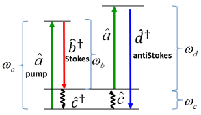
Figure 1: (Color online) Two-photon stimulated Raman scheme. The pump photon is converted into a Stokes photon and a phonon. The pump photon can also mix with a phonon to produce an anti-Stokes photon.

Here it is worthy to note that V Per̆inová et al. perinova have recently studied the possibility of observing entanglement in Raman process using the method of invariant subspace. They have followed an independent approach and have numerically computed the time dependence of a measure of entanglement. Earlier S V Kuznetsov et al. kuznetsov studied the entanglement in the stimulated Raman process considering only two modes (Stokes mode and phonon mode) and taking the pump mode as the classical light source. Naturally Kuznetsov et al.’s work illustrated an incomplete scenario and failed to observe intermodal entanglement involving anti-Stokes mode and pump mode. To circumvent this limitation we have used here a completely quantum mechanical Hamiltonian. Further, Pathak, K$\breve{\mathrm{r}}$epelka and Per̆ina Anirban with Perina have recently investigated the possibilities of observing intermodal entanglement in the Raman processes using the same Hamiltonian but with a short-time approximated solution. Their work is restricted by the intrinsic limitations of the short-time approximation. Such limitations may be circumvented by the analytical methods developed by us in recent past to study the stimulated Raman scheme bsen1 -bsen4 . Those methods are systematically used here and a relatively complete scenario of intermodal entanglement in Raman processes is presented here. Interestingly, we have observed intermodal entanglement between i) pump mode and anti-Stokes mode, and ii) Stokes mode and anti-stokes mode. These two intermodal entanglement was not observed in the earlier analytic studies kuznetsov ; Anirban with Perina . The beauty of the present study lies in the fact that analytic expressions for separability criterion are obtained by a completely quantum mechanical treatment where all four modes are considered quantum mechanical. If we look closely into the methodology adopted in the earlier studies we would quickly find that the approach adopted in the present paper is simpler and easily extensible to the other physical systems which are described by bosonic Hamiltonians.

The paper is organized as follows. In the Section II we have described the Hamiltonian of spontaneous and stimulated Raman processes and its operator solution. In Section III we have used the solution to show that it is possible to observe intermodal entanglement in Raman processes. The inseparability criteria used for this purpose are also described in this section. Finally, Section IV is dedicated to conclusions where we have briefly summarized the result of the present study and have also discussed the mutual relations among different nonclassical phenomena observed in the Raman processes.

II Model Hamiltonian

The Hamiltonian szlachetka1 -bsen4 , walls of our interest is

$$\begin{array}[]{lcl}H&=&\omega_{a}a^{\dagger}a+\omega_{b}b^{\dagger}b+\omega_{c}c^{\dagger}c+\omega_{d}d^{\dagger}d\\ &+&g\left(ab^{\dagger}c^{\dagger}+h.c.\right)+\chi\left(acd^{\dagger}+\mathrm{h.c.}\right),\end{array}$$ (1)

where h.c. stands for the Hermitian conjugate. Throughout the present paper, we use $\hbar=1$. The annihilation (creation) operators $a(a^{\dagger}),\,b(b^{\dagger}),\,c\left(c^{\dagger}\right),\,d(d^{\dagger})$ correspond to the laser (pump) mode, Stokes mode, vibration (phonon) mode and anti-Stokes mode, respectively. They obey the well-known boson commutation relations. The quantities $\omega_{a}$, $\omega_{b}$, $\omega_{c}$ and $\omega_{d}$ correspond to the frequencies of pump mode $a$, Stokes mode $b$, vibration (phonon) mode $c$ and anti-Stokes mode $d$, respectively. The parameters $g$ and $\chi$ are the Stokes and anti-Stokes coupling constants, respectively. Coupling constant $g$ ($\chi$) denotes the strength of coupling between the Stokes (anti-Stokes) mode and the vibrational (phonon) mode and depends on the actual interaction mechanism. The dimension of $g$ and $\chi$ are that of frequency and consequently $gt$ and $\chi t$ are dimensionless. Further, $gt$ and $\chi t$ are very small compared to unity. In order to study the possibility of intermodal entanglement, we need simultaneous solutions of the following Heisenberg operator equations of motion for various field operators

$$\begin{array}[]{lcl}\dot{a}&=&-i\left(\omega_{a}a+gbc+\chi cd\right)\\ \dot{b}&=&-i\left(\omega_{b}b+gac^{\dagger}\right)\\ \dot{c}&=&-i\left(\omega_{c}c+gab^{\dagger}+\chi a^{\dagger}d\right)\\ \dot{d}&=&-\left(\omega_{d}d+\chi ac\right).\end{array}$$ (2)

The above set of coupled nonlinear differential operator equations (2) are not exactly solvable in the closed analytical form under weak pump condition. But when the pump is very strong the operator $a$ can be replaced by a $c$-number and the above set of equations (2) can be solved exactly perina . In order to solve these equations under weak pump approximation we use the perturbative approach. Our solutions are more general than the well-known short-time approximation. Details of the calculations are given in our previous papers bsen1 - bsen4 . Here we just note that under weak pump approximation, the solutions of Eq. (2) assume the following form:

$$\begin{array}[]{lcl}a(t)&=&f_{1}a(0)+f_{2}b(0)c(0)+f_{3}c^{\dagger}(0)d(0)+f_{4}a^{\dagger}(0)b(0)d(0)+f_{5}a(0)b(0)b^{\dagger}(0)\\ &+&f_{6}a(0)c^{\dagger}(0)c(0)+f_{7}a(0)c^{\dagger}(0)c(0)+f_{8}a(0)d^{\dagger}(0)d(0)\\ b(t)&=&g_{1}b(0)+g_{2}a(0)c^{\dagger}(0)+g_{3}a^{2}(0)d^{\dagger}(0)+g_{4}c^{\dagger^{2}}(0)d(0)+g_{5}b(0)c(0)c^{\dagger}(0)\\ &+&g_{6}b(0)a(0)a^{\dagger}(0)\\ c(t)&=&h_{1}c(0)+h_{2}a(0)b^{\dagger}(0)+h_{3}a^{\dagger}(0)d(0)+h_{4}b^{\dagger}(0)c^{\dagger}(0)d(0)+h_{5}c(0)a(0)a^{\dagger}(0)\\ &+&h_{6}c(0)b(0)b^{\dagger}(0)+h_{7}c(0)d^{\dagger}(0)d(0)+h_{8}c(0)a^{\dagger}(0)a(0)\\ d(t)&=&l_{1}d(0)+l_{2}a(0)c(0)+l_{3}a^{2}(0)b^{\dagger}(0)+l_{4}b(0)c^{2}(0)+l_{5}c^{\dagger}(0)c(0)d(0)\\ &+&l_{6}a(0)a^{\dagger}(0)d(0)\end{array}.$$ (3)

The functions $f_{i},\,g_{i},\,h_{i}$ and $l_{i}$ are evaluated from the dynamics under the initial conditions. In order to apply the boundary condition, we put $t=0$, in the first term of the Eq. (3). It is clear that $f_{1}(0)=g_{1}(0)=h_{1}(0)=l_{1}(0)=1$ and $f_{i}(0)=g_{i}(0)=h_{i}(0)=l_{i}(0)=0$ (for $i=2,\,3,\,4,\,5,\,6,\,7$ and $8$). Under these initial conditions the corresponding solutions for $f_{i}(t),\,g_{i}(t),\,h_{i}(t)$ and $l_{i}(t)$ are obtained as given in the Appendix.

The solutions Eqs. (3), (38)-(50) are valid up to the second orders in $g$ and $\chi$. Interestingly, there is no restriction on time $t$. For example, $f_{2}$ rises indefinitely with the increase of time $t.$ Clearly, the divergent nature of the parameters $f_{i},\,g_{i},\,h_{i}$ and $l_{i}$ become more explicit as the order of the perturbation theory is increased. The secular nature is a direct outcome of the perturbation theory. In the present investigation the secular term is not a problem since we consider small interaction time. Small interaction time also ensures that the damping term contributes insignificantly. Here $\Delta\omega_{1}=\omega_{b}+\omega_{c}-\omega_{a}$ and $\Delta\omega_{2}=\omega_{a}+\omega_{c}-\omega_{d}$. Normally, the detunings $\Delta\omega_{1}$ and $\Delta\omega_{2}$ are extremely small. In the present investigation, we however assume that the small (non-zero) detuning is present and hence $\Delta\omega_{1}\neq 0$ and $\Delta\omega_{2}\neq 0.$ Here we have used $|\Delta\omega_{1}|=0.1$ MHz and $|\Delta\omega_{2}|=0.19$ MHz. Of course, in Eqs. (38)-(50) we have neglected the terms beyond the second order in $g$ and $\chi.$ Now we may use Eq. (3) to obtain the temporal evolution of the number operators of various modes as

$$\begin{array}[]{lcl}N_{a}(t)&=&|f_{1}|^{2}a^{\dagger}(0)a(0)+|f_{2}|^{2}b^{\dagger}(0)c^{\dagger}(0)b(0)c(0)+|f_{3}|^{2}c(0)d(0)^{\dagger}c^{\dagger}(0)d(0)\\ &+&\left[f_{1}^{\ast}f_{2}a^{\dagger}(0)b(0)c(0)+\right.f_{1}^{\ast}f_{3}a^{\dagger}(0)c^{\dagger}(0)d(0)+f_{1}^{\ast}f_{4}a^{\dagger}(0)a^{\dagger}(0)b(0)d(0)\\ &+&f_{1}^{\ast}f_{5}(a^{\dagger}(0)a(0)+a^{\dagger}(0)a(0)b^{\dagger}(0)b(0))+f_{1}^{\ast}f_{6}a^{\dagger}(0)a(0)c^{\dagger}(0)c(0)\\ &+&f_{1}^{\ast}f_{7}a^{\dagger}(0)a(0)c^{\dagger}(0)c(0)+f_{1}^{\ast}f_{8}a^{\dagger}(0)a(0)d^{\dagger}(0)d(0)\\ &+&\left.f_{2}^{\ast}f_{3}b^{\dagger}(0)c^{\dagger^{2}}(0)d(0)+\mathrm{h.c.}\right],\end{array}$$ (4)

$$\begin{array}[]{lcl}N_{b}(t)&=&|g_{1}|^{2}b^{\dagger}(0)b(0)+|g_{2}|^{2}a^{\dagger}(0)c(0)a(0)c^{\dagger}(0)+\left[g_{1}^{*}g_{2}b^{\dagger}(0)a(0)c^{\dagger}(0)\right.\\ &+&g_{1}^{*}g_{3}b^{\dagger}(0)a^{2}(0)d^{\dagger}(0)+g_{1}^{*}g_{4}b^{\dagger}(0)c^{\dagger^{2}}(0)d(0)+g_{1}^{*}g_{5}(b^{\dagger}(0)b(0)\\ &+&b^{\dagger}(0)b(0)c^{\dagger}(0)c(0))+g_{1}^{*}g_{6}(b^{\dagger}(0)b(0)+b^{\dagger}(0)b(0)a^{\dagger}(0)a(0))\\ &+&\left.\mathrm{h.c.}\right],\end{array}$$ (5)

$$\begin{array}[]{ccl}N_{c}(t)&=&|h_{1}|^{2}c^{\dagger}(0)c(0)+|h_{2}|^{2}a^{\dagger}(0)b(0)a(0)b^{\dagger}(0)+|h_{3}|^{2}a(0)d^{\dagger}(0)a^{\dagger}(0)d(0)\\ &+&\left[h_{1}^{*}h_{2}c^{\dagger}(0)a(0)b^{\dagger}(0)+h_{1}^{*}h_{3}c^{\dagger}(0)a^{\dagger}(0)d(0)\right.\\ &+&h_{1}^{*}h_{4}c^{\dagger}(0)b^{\dagger}(0)c^{\dagger}(0)d(0)+h_{1}^{*}h_{5}(c^{\dagger}(0)c(0)+c^{\dagger}(0)c(0)a^{\dagger}(0)a(0))\\ &+&h_{1}^{*}h_{6}(c^{\dagger}(0)c(0)+c^{\dagger}(0)c(0)b^{\dagger}(0)b(0))+h_{1}^{*}h_{7}c^{\dagger}(0)c(0)d^{\dagger}(0)d(0)\\ &+&\left.h_{1}^{*}h_{8}c^{\dagger}(0)c(0)a^{\dagger}(0)a(0)+h_{2}^{*}h_{3}a^{\dagger^{2}}(0)b(0)d(0)+\mathrm{h.c.}\right],\end{array}$$ (6)

and

$$\begin{array}[]{lcl}N_{d}(t)&=&|l_{1}|^{2}d^{\dagger}(0)d(0)+|l_{2}|^{2}a^{\dagger}(0)a(0)c^{\dagger}(0)c(0)+\left[l_{1}^{\ast}l_{2}a(0)c(0)d^{\dagger}(0)\right.\\ &+&l_{1}^{\ast}l_{3}a^{2}(0)b^{\dagger}(0)d^{\dagger}(0)+l_{1}^{\ast}l_{4}b(0)c^{2}(0)d^{\dagger}(0)+l_{1}^{\ast}l_{5}c^{\dagger}(0)c(0)d^{\dagger}(0)d(0)\\ &+&\left.l_{1}^{\ast}l_{6}d^{\dagger}(0)d(0)(1+a^{\dagger}(0)a(0))+\mathrm{h.c.}\right].\end{array}.$$ (7)

In the following section these number operators will be used to study the intermodal entanglement in Raman processes.

III Intermodal entanglement

In order to investigate the intermodal entanglement for various coupled modes, we assume that all photon and phonon modes are initially coherent. In other words, the composite boson field consisting of photons and phonon are in the initial coherent state. Therefore, the composite coherent state arises from the product of the coherent states $|\alpha_{1}\rangle,\,|\alpha_{2}\rangle$, $|\alpha_{3}\rangle,$ and $|\alpha_{4}\rangle$ which are the eigenkets of $a,\,b,\,c$ and $d$ respectively. Thus the initial composite state is

$$|\psi(0)\rangle=|\alpha_{1}\rangle\otimes|\alpha_{2}\rangle\otimes|\alpha_{3}\rangle\otimes|\alpha_{4}\rangle.$$ (8)

It is clear that the initial state is separable. Now the field operator $a(t)$ operating on such a multi-mode coherent state gives rise to the complex eigenvalue $\alpha_{1}(t).$ Hence we have,

$$a(0)|\psi(0)\rangle=\alpha_{1}|\psi(0)\rangle,$$ (9)

where $|\alpha_{1}|^{2}$ is the number of input photons in the pump mode $a.$ In a similar fashion we have three more complex amplitudes $\alpha_{2}(t)$, $\alpha_{3}(t)$ and $\alpha_{4}(t)$ corresponding to the Stokes, vibrational (phonon) and anti-Stokes field mode operators $b,$ $c$ and $d$ respectively. Clearly, for a spontaneous process, the complex amplitudes are $\alpha_{2}=\alpha_{3}=\alpha_{4}=0$ and $\alpha_{1}\neq 0.$ For partial spontaneous process, the complex amplitude $\alpha_{1}$ and any one of the remaining three eigenvalues are not equal to zero while the other two complex amplitudes are zero. On the other hand, for a stimulated process, the complex amplitudes are not necessarily zero. In our present investigation we consider $\alpha_{1}=\left|\alpha_{1}\right|e^{-i\phi}$ and the other eigenvalues for the Stokes, vibrational (phonon) and anti-Stokes field modes are real. The aim of the present work is to investigate the possibility of intermodal entanglement in the spontaneous, partially spontaneous and stimulated Raman processes. To do so let us begin with the investigation of two mode entanglement using Hillery and Zubairy’s criteria.

III.1 Two mode entanglement

There are two criteria due to Hillery and Zubairy hz-prl -two-mode-citeria-hz . The first one is

$$\langle N_{a}N_{b}\rangle-|\langle ab^{\dagger}\rangle|^{2}<0.$$ (10)

On the other hand, the second criterion is given by

$$\langle N_{a}\rangle\langle N_{b}\rangle-|\langle ab\rangle|^{2}<0.$$ (11)

From here onward we will refer to these criteria as HZ-1 and HZ-2 criterion respectively. In addition to these two criteria, we will also use the Duan’s inseparability criterion due to Duan et al. duan :

$$\langle\Delta a^{\dagger}\Delta a\rangle\langle\Delta b^{\dagger}\Delta b\rangle-|\langle\Delta a\Delta b\rangle|^{2}<0.$$ (12)

In the criteria Eqs. (10)-(12), $a$ and $b$ are annihilation operators for two arbitrary modes. They are not limited to the pump mode and the Stokes mode only.

We note that all the above criteria are only sufficient (not necessary) for detection of entanglement. Keeping this fact in mind, we have applied all these criteria to study intermodal entanglement between different modes of Raman Hamiltonian and have observed intermodal entanglement in various situations.

Let us first investigate the possibility of two mode entanglement in Raman process using HZ-1 criterion. From Eqs. (3), (4), (5) and (8) we obtain

$$\begin{array}[]{lcl}\left\langle N_{a}N_{b}\right\rangle-\left|\left\langle ab^{\dagger}\right\rangle\right|^{2}&=&\left|f_{3}\right|^{2}\left|\alpha_{2}\right|^{2}\left|\alpha_{4}\right|^{2}\\ &+&\left|g_{2}\right|^{2}\left(\left|\alpha_{1}\right|^{4}-\left|\alpha_{1}\right|^{2}\left|\alpha_{2}\right|^{2}\right).\end{array}$$ (13)

Consequently, for spontaneous Raman process Eq. (13) reduces to

$$\begin{array}[]{lcl}\left\langle N_{a}N_{b}\right\rangle-\left|\left\langle ab^{\dagger}\right\rangle\right|^{2}&=&\left|g_{2}\right|^{2}\left|\alpha_{1}\right|^{4}\end{array}$$ (14)

It is evidently clear that the right hand side of the Eq. (14) is always positive. Hence HZ-1 criterion does not show any signature of intermodal entanglement between pump and Stokes modes in the spontaneous Raman process. For partially spontaneous Raman process ($|\alpha_{1}|\neq 0,\,|\alpha_{2}|\neq 0,\,|\alpha_{3}|=|\alpha_{4}|=0$), the Eq. (13) reduces to

$$\left\langle N_{a}N_{b}\right\rangle-\left|\left\langle ab^{\dagger}\right\rangle\right|^{2}=\left|g_{2}\right|^{2}\left(\left|\alpha_{1}\right|^{2}-\left|\alpha_{2}\right|^{2}\right)\left|\alpha_{1}\right|^{2}.$$ (15)

It is clear that the entanglement is possible in the partially spontaneous Raman process only when $\left|\alpha_{2}\right|^{2}>\left|\alpha_{1}\right|^{2}$, i.e. the number of Stokes photon is more than the number of pump photons, which is not the usual case. According to the HZ-1 criterion of Eq. (10), it is clear that the negative values on the right hand side of Eq. (13) would indicate the presence of intermodal entanglement between the pump mode and the Stokes mode in stimulated Raman process. To investigate the possibility of intermodal entanglement in the stimulated Raman process we have used $\chi=g=10^{5}$ Hz, $|\alpha_{1}|=10,$ $|\alpha_{2}|=8,$ $|\alpha_{3}|=0.01$ and $|\alpha_{4}|=1$ foot2 . We have plotted the right hand side of (13) in Fig. 2a which does not show any signature of intermodal entanglement between pump mode and the Stokes mode in the stimulated Raman process.

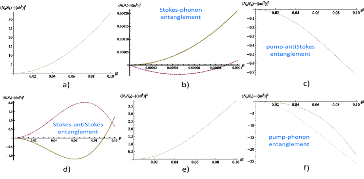
Figure 2: (Color online) Intermodal entanglement in stimulated Raman process by using HZ-1 criterion: The dotted line, dash-dotted line and the smooth line are used for the phase angle of the input complex amplitude $\alpha_{1}$ for $\phi=0,$ $\pi$and $\pi/2$ respectively. a) intermodal entanglement is observed between Stokes mode and vibration-phonon mode for $\phi=\pi/2$, b) intermodal entanglement is observed between pump mode and anti-Stokes mode, c) intermodal entanglement is observed between Stokes mode and anti-Stokes mode for $\phi=0$ and $\pi/2$, d) signature of intermodal entanglement is not observed between vibration-phonon mode and anti-Stokes mode, e) intermodal entanglement is observed between pump mode and vibration-phonon mode.

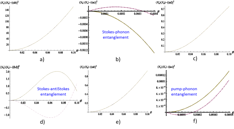
Figure 3: (Color online) Intermodal entanglement in stimulated Raman process by using HZ-2 criterion: The dotted line, dash-dotted line and the smooth line are used for the phase angle of the input complex amplitude $\alpha_{1}$ for $\phi=0,$ $\pi/2$ and $\pi$ respectively. a) intermodal entanglement is not observed between Stokes mode and pump mode b) intermodal entanglement is observed between Stokes mode and vibration-phonon mode, c) signature of intermodal entanglement is not observed between pump mode and anti-Stokes mode, d) intermodal entanglement is observed between Stokes mode and anti-Stokes mode only for $\phi=\pi/2$, e) intermodal entanglement is not observed between vibration-phonon mode and anti-Stokes mode, f) intermodal entanglement (time dependent) is observed between pump mode and vibration-phonon mode for $\phi=\pi/2$.

Here we would like to note that once we have an analytic expression for the HZ-1 or HZ-2 or Duan criteria in stimulated Raman process, it is straightforward to study the special cases of: i) spontaneous Raman process, where $\alpha_{2}=\alpha_{3}=\alpha_{4}=0$ but $\alpha_{1}\neq 0$ and ii) partial spontaneous Raman process, where $\alpha_{1}\neq 0$ and any one of the other three $\alpha_{i}\,(i=2,\,3,\,4)$ is non-zero.

The same technique used in the above case is now adopted to obtain the following equations for the study of intermodal entanglement in stimulated Raman process using HZ-1 criterion:

$$\begin{array}[]{lcl}\left\langle N_{b}N_{c}\right\rangle-\left|\left\langle bc^{\dagger}\right\rangle\right|^{2}&=&\left|g_{2}\right|^{2}\left(3\left|\alpha_{1}\right|^{2}\left|\alpha_{3}\right|^{2}+3\left|\alpha_{1}\right|^{2}\left|\alpha_{2}\right|^{2}+\left|\alpha_{1}\right|^{2}-\left|\alpha_{2}\right|^{2}\left|\alpha_{3}\right|^{2}\right)+\left|h_{3}\right|^{2}\left|\alpha_{2}\right|^{2}\left|\alpha_{4}\right|^{2}\\ &+&\left[\left\{h_{1}^{*}h_{2}\alpha_{1}\alpha_{2}^{*}\alpha_{3}^{*}+2g_{4}^{*}g_{1}\alpha_{2}\alpha_{3}^{2}\alpha_{4}^{*}+h_{2}h_{3}^{*}\alpha_{1}^{2}\alpha_{2}^{*}\alpha_{4}^{*}\right\}+{\rm c.c.}\right]\end{array}$$ (16)

$$\begin{array}[]{lcl}\left\langle N_{a}N_{d}\right\rangle-\left|\left\langle ad^{\dagger}\right\rangle\right|^{2}&=&\left|f_{3}\right|^{2}\left(\left|\alpha_{3}\right|^{2}+\left|\alpha_{4}\right|^{4}+\left|\alpha_{1}\right|^{2}\left|\alpha_{3}\right|^{2}-\left|\alpha_{1}\right|^{2}\left|\alpha_{4}\right|^{2}\right)-\left|l_{2}\right|^{2}\left(\left|\alpha_{3}\right|^{2}+\left|\alpha_{1}\right|^{2}\left|\alpha_{3}\right|^{2}\right)\end{array}$$ (17)

$$\begin{array}[]{lcl}\left\langle N_{b}N_{d}\right\rangle-\left|\left\langle bd^{\dagger}\right\rangle\right|^{2}&=&\left|g_{2}\right|^{2}\left|\alpha_{1}\right|^{2}\left|\alpha_{4}\right|^{2}+\left[\left\{l_{1}^{*}l_{3}\alpha_{1}^{2}\alpha_{2}^{*}\alpha_{4}^{*}+{\rm c.c.}\right\}\right]\end{array}$$ (18)

$$\begin{array}[]{lcl}\left\langle N_{c}N_{d}\right\rangle-\left|\left\langle cd^{\dagger}\right\rangle\right|^{2}&=&\left|l_{2}\right|^{2}\left(2\left|\alpha_{1}\right|^{2}+2\left|\alpha_{1}\right|^{2}\left|\alpha_{4}\right|^{2}-2\left|\alpha_{4}\right|^{2}-\left|\alpha_{4}\right|^{4}-\left|\alpha_{3}\right|^{2}\left|\alpha_{4}\right|^{2}\right)+\left|h_{2}\right|^{2}\left|\alpha_{1}\right|^{2}\left|\alpha_{4}\right|^{2}\end{array}$$ (19)

$$\begin{array}[]{lcl}\left\langle N_{a}N_{c}\right\rangle-\left|\left\langle ac^{\dagger}\right\rangle\right|^{2}&=&\left|f_{2}\right|^{2}\left(2\left|\alpha_{1}\right|^{2}+\left|\alpha_{1}\right|^{4}+\left|\alpha_{1}\right|^{2}\left|\alpha_{3}\right|^{2}-4\left|\alpha_{2}\right|^{2}-2\left|\alpha_{1}\right|^{2}\left|\alpha_{2}\right|^{2}-2\left|\alpha_{2}\right|^{2}\left|\alpha_{3}\right|^{2}\right)\\ &+&\left|f_{3}\right|^{2}\left(\left|\alpha_{4}\right|^{2}+3\left|\alpha_{3}\right|^{2}\left|\alpha_{4}\right|^{2}+3\left|\alpha_{1}\right|^{2}\left|\alpha_{4}\right|^{2}-\left|\alpha_{1}\right|^{2}\left|\alpha_{3}\right|^{2}\right)+\left[\left\{f_{1}^{\ast}f_{3}\alpha_{1}^{\ast}\alpha_{3}^{\ast}\alpha_{4}\right.\right.\\ &+&\left.\left.h_{2}^{\ast}h_{3}\alpha_{1}^{\ast 2}\alpha_{2}\alpha_{4}+f_{2}^{\ast}f_{3}\alpha_{2}^{\ast}\alpha_{3}^{\ast 2}\alpha_{4}\right\}+{\rm c.c.}\right].\end{array}$$ (20)

The right hand sides (RHS) of Eqs. (16)-(20) are plotted in Fig. 2b - Fig. 2f. It is interesting to note that the presence of intermodal entanglement in stimulated Raman process is observed between i) the Stokes mode and the vibration (phonon) mode (Fig. 2b), ii) the pump mode and the anti-Stokes mode (Fig. 2c), iii) the Stokes mode and the anti-Stokes mode (Fig. 2d) and iv) the pump mode and vibration mode (Fig. 2f). However, no signature of intermodal entanglement is observed in the other two cases (Figs. 2a and e). Further, it does not show the presence of genuine entanglement between any three modes of the system. Interestingly, with the suitable choice of the complex eigenvalues $\alpha_{i}$ it is possible to observe the signature of the intermodal entanglement using HZ-1 criteria in partially spontaneous Raman process in several ways but no such signature is observed for the completely spontaneous Raman process.

Since the HZ-1 criterion is only sufficient, we might have failed to detect some intermodal entanglement. In an attempt to detect such intermodal entanglement using HZ-2 criterion (11), we have used Eqs. (3), (4)-(7) and (8) to yield:

$$\begin{array}[]{lcl}\left\langle N_{a}\right\rangle\left\langle N_{b}\right\rangle-\left|\left\langle ab\right\rangle\right|^{2}&=&\left|g_{2}\right|^{2}\left|\mbox{$\alpha$}_{1}\right|^{4}+\left|f_{3}\right|^{2}\left|\mbox{$\alpha$}_{2}\right|^{2}\left|\mbox{$\alpha$}_{4}\right|^{2}-\left[\left(g_{1}^{\ast}g_{6}\right.\right.\\ &+&\left.\left.f_{1}^{\ast}f_{2}g_{1}^{\ast}g_{2}\right)\left|\mbox{$\alpha$}_{1}\right|^{2}\left|\mbox{$\alpha$}_{2}\right|^{2}+c.c.\right]\end{array},$$ (21)

and

$$\begin{array}[]{lcl}\left\langle N_{b}\right\rangle\left\langle N_{c}\right\rangle-\left|\left\langle bc\right\rangle\right|^{2}&=&\left|g_{2}\right|^{2}\left|\mbox{$\alpha$}_{1}\right|^{2}\left|\mbox{$\alpha$}_{3}\right|^{2}-\left|h_{2}\right|^{2}\left(1+\left|\mbox{$\alpha$}_{2}\right|^{2}\right)\left|\mbox{$\alpha$}_{1}\right|^{2}+\left|h_{3}\right|^{2}\left|\mbox{$\alpha$}_{2}\right|^{2}\left|\mbox{$\alpha$}_{4}\right|^{2}\\ &-&\left[\left(h_{1}^{*}h_{2}\alpha_{1}\alpha_{2}^{*}\alpha_{3}^{*}+\left(h_{1}h_{4}^{*}+g_{1}g_{2}^{*}h_{1}h_{3}^{*}\right)\alpha_{2}\alpha_{3}^{2}\alpha_{4}^{*}+h_{2}^{*}h_{3}\alpha_{1}^{*2}\alpha_{2}\alpha_{4}\right.\right.\\ &+&\left.\left.h_{1}^{*}h_{6}\left|\mbox{$\alpha$}_{2}\right|^{2}\left|\mbox{$\alpha$}_{3}\right|^{2}+g_{1}g_{2}^{*}h_{1}^{*}h_{2}\left|\mbox{$\alpha$}_{1}\right|^{2}\left|\mbox{$\alpha$}_{3}\right|^{2}\right)+c.c.\right],\end{array}$$ (22)

$$\begin{array}[]{lcl}\left\langle N_{a}\right\rangle\left\langle N_{d}\right\rangle-\left|\left\langle ad\right\rangle\right|^{2}&=&\left|f_{3}\right|^{2}\left|\alpha_{4}\right|^{4}-\left[l_{1}^{*}l_{6}\left|\mbox{$\alpha$}_{1}\right|^{2}\left|\mbox{$\alpha$}_{4}\right|^{2}+c.c\right],\end{array}$$ (23)

$$\begin{array}[]{lcl}\left\langle N_{b}\right\rangle\left\langle N_{d}\right\rangle-\left|\left\langle bd\right\rangle\right|^{2}&=&\left|g_{2}\right|^{2}\left|\alpha_{1}\right|^{2}\left|\alpha_{4}\right|^{2}-\left[l_{1}^{*}l_{3}\alpha_{1}^{2}\alpha_{2}^{*}\alpha_{4}^{*}+c.c\right],\end{array}$$ (24)

$$\begin{array}[]{lcl}\left\langle N_{c}\right\rangle\left\langle N_{d}\right\rangle-\left|\left\langle cd\right\rangle\right|^{2}&=&\left|h_{2}\right|^{2}\left|\mbox{$\alpha$}_{1}\right|^{2}\left|\mbox{$\alpha$}_{4}\right|^{2}+\left|h_{3}\right|^{2}\end{array}\left|\mbox{$\alpha$}_{4}\right|^{4}-\left[l_{1}^{*}l_{5}\left|\mbox{$\alpha$}_{3}\right|^{2}\left|\mbox{$\alpha$}_{4}\right|^{2}+c.c\right],$$ (25)

$$\begin{array}[]{lcl}\left\langle N_{a}\right\rangle\left\langle N_{c}\right\rangle-\left|\left\langle ac\right\rangle\right|^{2}&=&\left|h_{2}\right|^{2}\left|\mbox{$\alpha$}_{1}\right|^{4}-\left|h_{3}\right|^{2}\left(\left|\mbox{$\alpha$}_{4}\right|^{2}+\left|\mbox{$\alpha$}_{1}\right|^{2}\left|\mbox{$\alpha$}_{4}\right|^{2}\right)+\left|f_{3}\right|^{2}\left|\mbox{$\alpha$}_{3}\right|^{2}\left|\mbox{$\alpha$}_{4}\right|^{2}-\left[\left(h_{1}^{\ast}h_{3}\alpha_{1}^{\ast}\alpha_{3}^{\ast}\alpha_{4}\right.\right.\\ &+&h_{1}^{\ast}h_{8}\left|\mbox{$\alpha$}_{1}\right|^{2}\left|\mbox{$\alpha$}_{3}\right|^{2}+h_{2}^{\ast}h_{3}\alpha_{1}^{\ast 2}\alpha_{2}\alpha_{4}-h_{1}^{\ast}h_{5}\left|\mbox{$\alpha$}_{1}\right|^{2}\left|\mbox{$\alpha$}_{3}\right|^{2}\\ &+&\left.\left.f_{1}^{\ast}f_{2}h_{3}^{\ast}h_{1}\alpha_{2}\alpha_{3}^{2}\alpha_{4}^{\ast}+f_{1}^{\ast}f_{3}h_{3}^{\ast}h_{1}\left|\mbox{$\alpha$}_{3}\right|^{2}\left|\mbox{$\alpha$}_{4}\right|^{2}\right)+c.c.\right].\end{array}$$ (26)

From the closed form analytic expressions Eqs. (21)-(26), it is possible to obtain the signature of intermodal entanglement in various cases. Interestingly, we obtain intermodal entanglement between Stokes mode and vibration mode for spontaneous Raman process. The intermodal entanglement Eqs. (21)-(26) for stimulated Raman processes are illustrated in the Fig. 3a-Fig. 3f. In accordance to HZ-2 criterion, negative values of the ordinates indicate the signature of entanglement. Therefore, the intermodal entanglement is observed in: i) Stokes mode and vibration mode, ii) Stokes mode and anti-Stokes mode and iii) pump mode and vibration mode. However, there is no signature of intermodal entanglement in the remaining cases for Stimulated Raman processes. It is possible to obtain the intermodal entanglement for various partially spontaneous Raman processes. However, these results are not exhibited in the present text. It is interesting to note that HZ-2 criterion failed to detect intermodal entanglement between, pump and anti-Stokes mode. Thus the Raman process provides a very nice example of physical system where it can be shown with physical example that these inseparability criteria are only sufficient. Still there are two situations where we have not found the signature of intermodal entanglement. Let us see what happens when we apply another sufficient but not necessary criterion of inseparability.

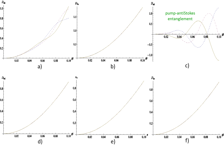
Figure 4: (Color online) Intermodal entanglement in stimulated Raman process by using Duan criterion: The dotted line, dash-dotted line and the smooth line are used for the phase angle of the input complex amplitude $\alpha_{1}$ for $\phi=0,$ $\pi/2$ and $\pi$ respectively. Intermodal entanglement is only observed between pump mode and anti-Stokes mode (Fig.4.(c)).

Now Duan criterion Eq. (12) for the intermodal entanglement can also be written as shivkumar

$$\begin{array}[]{lcl}D=\left\langle\left(\Delta u\right)^{2}\right\rangle+\left\langle\left(\Delta v\right)^{2}\right\rangle&-2<&0\end{array}$$ (27)

where

$$\begin{array}[]{lcl}\hat{u}&=&\frac{1}{\sqrt{2}}\left[\left(a+a^{\dagger}\right)+\left(b+b^{\dagger}\right)\right]\end{array}$$ (28)

and

$$\begin{array}[]{lcl}\hat{v}&=&\frac{1}{i\sqrt{2}}\left[\left(a-a^{\dagger}\right)+\left(b-b^{\dagger}\right)\right]\end{array}.$$ (29)

Using Eqs. (3), (8) and (27)-(29) we can obtain analytic expression for $D$ the left hand side of Duan et al. criterion Eq. (27),

For mode $a$ and $b$,

$$\begin{array}[]{lcl}D_{ab}&=&2\left[\left|f_{3}\right|\left|\alpha_{4}\right|^{2}+\left|g_{2}\right|^{2}\left|\alpha_{1}\right|^{2}\right.\\ &+&\frac{1}{2}\left\{\left(f_{1}g_{6}^{\ast}+f_{5}g_{1}^{\ast}\right)\alpha_{1}\alpha_{2}^{\ast}\right.\\ &+&\left.\left.\left(2f_{1}g_{3}^{\ast}+f_{4}g_{1}^{\ast}+f_{3}g_{2}^{\ast}\right)\alpha_{1}^{\ast}\alpha_{4}+\mathrm{c.c.}\right\}\right],\end{array}$$ (30)

for mode $a$ and $c$

$$\begin{array}[]{lcl}D_{ac}&=&2\left[\left|f_{3}\right|\left|\alpha_{4}\right|^{2}+\left|h_{2}\right|^{2}\left|\alpha_{1}\right|^{2}+\left|h_{3}\right|^{2}\left|\alpha_{4}\right|^{2}\right.\\ &+&\frac{1}{2}\left\{\left(f_{1}h_{5}^{\ast}+f_{6}h_{1}^{\ast}+f_{3}h_{3}^{\ast}\right.\right.\\ &+&\left.\left.\left.f_{7}h_{1}^{\ast}+f_{1}h_{8}^{\ast}\right)\alpha_{1}\alpha_{3}^{\ast}\right\}+\mathrm{c.c.}\right],\end{array}$$ (31)

for mode $b$ and $c$

$$\begin{array}[]{lcl}D_{bc}&=&2\left[\left|g_{2}\right|^{2}\left|\alpha_{1}\right|^{2}+\left|h_{2}\right|^{2}\left|\alpha_{1}\right|^{2}+\left|h_{3}\right|^{2}\left|\alpha_{4}\right|^{2}\right.\\ &+&\left.\frac{1}{2}\left\{\left(g_{1}h_{6}^{\ast}+g_{5}h_{1}^{\ast}+g_{2}h_{2}^{\ast}\right)\alpha_{3}^{\ast}\alpha_{2}\right\}+\mathrm{c.c.}\right],\end{array}$$ (32)

for mode $a$ and $d$

$$\begin{array}[]{lcl}D_{ad}&=&2\left[\left|f_{3}\right|\left|\alpha_{4}\right|^{2}+\frac{1}{2}\left\{\left(f_{1}l_{2}^{\ast}+f_{3}l_{1}^{\ast}\right)\alpha_{3}^{\ast}\right.\right.\\ &+&\left.\left.\left(2f_{1}l_{3}^{\ast}+f_{4}l_{1}^{\ast}+f_{2}l_{2}^{\ast}\right)\alpha_{1}^{\ast}\alpha_{2}+f_{8}l_{1}^{\ast}\alpha_{1}\alpha_{4}^{\ast}+\mathrm{c.c.}\right\}\right],\end{array}$$ (33)

for mode $c$ and $d$

$$\begin{array}[]{lcl}D_{cd}&=&2\left[\left|h_{2}\right|^{2}\left|\alpha_{1}\right|^{2}+\left|h_{3}\right|^{2}\left|\alpha_{4}\right|^{2}+\right.\\ &+&\frac{1}{2}\left\{\left(2l_{4}h_{1}^{\ast}+l_{2}h_{2}^{\ast}+l_{1}h_{4}^{\ast}\right)\alpha_{2}\alpha_{3}\right.\\ &+&\left.\left.\left(l_{5}h_{1}^{\ast}+l_{1}h_{7}^{\ast}\right)\alpha_{3}^{\ast}\alpha_{4}++\mathrm{c.c.}\right\}\right],\end{array}$$ (34)

and for mode $b$ and $d$

$$\begin{array}[]{lcl}D_{bd}&=&2\left[\left|g_{2}\right|^{2}\left|\alpha_{1}\right|^{2}+\frac{1}{2}\left\{\left(l_{4}g_{1}^{\ast}+l_{2}g_{2}^{\ast}+l_{1}g_{4}^{\ast}\right)\alpha_{3}^{2}+\mathrm{c.c.}\right\}\right]\end{array}.$$ (35)

Right hand sides of equations (30)-(35) are plotted in Fig. 4a- Fig 4f. It is clear that the intermodal-entanglement is observed only between the pump mode and anti-Stokes mode. The criterion is non-conclusive in all other cases. This is so because Duan criterion is only sufficient.

inter-mode	HZ-1			HZ-2			Duan			antibunching bsen2	Squeezingbsen1
	$\phi=0$	$\pi/2$	$\pi$	$\phi=0$	$\pi/2$	$\pi$	$\phi=0$	$\pi/2$	$\pi$
$ab$	nc	nc	nc	nc	nc	nc	nc	nc	nc	possible	possible
$ac$	entangled	entangled	entangled	nc	entangled (time-dependent)	nc	nc	nc	nc	bunching	possible
$ad$	entangled	entangled	entangled	nc	nc	nc	entangled	nc	nc	anti-bunching	possible
$bc$	nc	entangled (time-dependent)	nc	entangled	nc	entangled	nc	nc	nc	bunching	possible
$bd$	entangled	nc	entangled	nc	entangled	nc	nc	nc	nc	antibunching	not possible
$cd$	nc	nc	nc	nc	nc	nc	nc	nc	nc	bunching	possible

Table 1: Relation between different nonclassical phenomena observed in stimulated Raman process. Here nc stands for non-conclusive. .

IV Conclusions

We have clearly established that the stimulated Raman process can produce intermodal entanglement. The observations are summarized in the Table 1. Here it would be apt to note that recently Pathak, $\mathrm{K}\breve{\mathrm{r}}\mathrm{epelka}$ and $\mathrm{Pe\breve{r}ina}$ Anirban with Perina have investigated the possibilities of observing intermodal entanglement in the Raman processes using a approximated short-time solution. They have identified intermodal entanglement in pump-phonon $ac$ and Stokes-phonon $bc$ modes only. However, in addition to those two modes we have observed intermodal entanglement in pump-antiStokes $ad$ and Stokes-antiStokes $bd$ modes too. In addition to these, we explore the various possibilities of getting intermodal entanglement in partial spontaneous Raman processes too. In this way, our solution is found more powerful compared to those of the solutions of Raman processes under short-time approximation. Further, the use of short-time solution led to the monotonic nature of entanglement parameter as seen in Eqs. (11) and (12) of ref. Anirban with Perina . As our solution is valid for all times and hence the entanglement parameters are free from this particular problem which is generally a characteristic of short-time solutions. Another earlier effort to study the intermodal entanglement in the Raman processes by S. V. Kuznetsov kuznetsov was restricted to the study of intermodal entanglement between Stokes mode and the vibration mode as they had considered a simplified two-mode Hamiltonian. Thus the use of a completely quantum mechanical description of the Raman process, our solution, and the strategy to use more than one inseparability criterion have helped us to obtain a relatively more complete picture of the intermodal entanglement in the Raman processes. Further, if we look at the possibilities of different kinds of nonclassicalities summarized in Table 1 (see the rows corresponding to $ac$, $bc$, and $bd$ modes), then we can quickly recognize that the existence of any one of the nonclassical phenomenon does not depend on the presence of the other. To be precise, entanglement, antibunching and squeezing are nonclassical phenomena but they are independent of each other. However, Duan criterion in the present form implies intermodal squeezing in one of the quadrature variable but the converse is not true. This fact can be clearly seen in the Table 1, where we note that except in $bd$ mode intermodal squeezing is possible in all other coupled modes. However, the Duan criterion of intermodal entanglement is satisfied only for the $ac$ mode.

In quantum optics, physical systems (matter-field interactions) are usually described by multi-mode bosonic Hamiltonians. The procedure followed in the present work may be applied directly to those systems to study the intermodal entanglement. It is expected that most of these systems will show intermodal entanglement. This is so because most of the quantum states are entangled. Separability is a very special case. A natural question should arise at this point: If entanglement is so common why are we looking for it? The answer lies in the fact that entanglement is one of the most important resources for quantum information processing and quantum communication but still it is not very easy to produce useful multi-partite entanglement. As many of the quantum optical systems described by bosonic Hamiltonian (including the system studied here) are experimentally achievable, useful intermodal entanglement may be produced by them. Entanglement obtained in such a system is expected to find application in controlled quantum teleportation, quantum information splitting, dense coding, direct secured quantum communication etc. We conclude this paper with an optimistic view that the present work will motivate others to look for theoretical and experimental generation of useful multi-mode entanglement in other quantum optical systems.

V ACKNOWLEDGMENTS

AP thanks Department of Science and Technology (DST), India for support provided through the DST project No. SR/S2/LOP-0012/2010 and he also thanks the Operational Program Education for Competitiveness - European Social Fund project CZ.1.07/2.3.00/20.0017 of the Ministry of Education, Youth and Sports of the Czech Republic. RO thanks the Ministry of Higher Education (MOHE)/University of Malaya HIR Grant No. A-000004-50001 for support.

Appendix A Parameters for the solutions in Eq. (3)

$$f_{1} = \exp(-i\omega_{a}t),$$

$$f_{2} = \frac{ge^{-i\omega_{a}t}}{\Delta\omega_{1}}\left[e^{-i\Delta\omega_{1}t}-1\right],$$

$$f_{3} = -\frac{\chi e^{-i\omega_{a}t}}{\Delta\omega_{2}}\left[e^{i\Delta\omega_{2}t}-1\right],$$

$$f_{4} = \begin{array}[]{l}-\frac{\chi ge^{-i\omega_{a}t}}{\Delta\omega_{1}}\left[\frac{e^{-i(\Delta\omega_{1}-\Delta\omega_{2})t}-1}{\Delta\omega_{1}-\Delta\omega_{2}}+\frac{e^{i\Delta\omega_{2}t}}{\Delta\omega_{2}}\right]\\ -\frac{\chi ge^{-i\omega_{a}t}}{\Delta\omega_{2}}\left[\frac{e^{-i(\Delta\omega_{1}-\Delta\omega_{2})t}-1}{\Delta\omega_{1}-\Delta\omega_{2}}-\frac{e^{-i\Delta\omega_{1}t}}{\Delta\omega_{1}}\right],\end{array}$$ (38)

$$f_{5} = \frac{g^{2}e^{-i\omega_{a}t}}{\Delta\omega_{1}^{2}}\left[e^{-i\Delta\omega_{1}t}-1\right]+\frac{ig^{2}te^{-i\omega_{a}t}}{\Delta\omega_{1}},$$

$$f_{6} = f_{5},$$

$$f_{7} = \frac{\chi^{2}e^{-i\omega_{a}t}}{\Delta\omega_{2}^{2}}\left[e^{i\Delta\omega_{2}t}-1\right]-\frac{i\chi^{2}te^{-i\omega_{a}t}}{\Delta\omega_{2}},$$

$$f_{8} = -f_{7}.$$

$$g_{1} = \exp(-i\omega_{b}t),$$

$$g_{2} = -\frac{ge^{-i\omega_{b}t}}{\Delta\omega_{1}}\left[e^{i\Delta\omega_{1}t}-1\right],$$

$$g_{3} = \begin{array}[]{l}\frac{\chi ge^{-i\omega_{b}t}}{\Delta\omega_{2}(\Delta\omega_{1}-\Delta\omega_{2})}\left[e^{i(\Delta\omega_{1}-\Delta\omega_{2})t}-1\right]\\ -\frac{\chi ge^{-i\omega_{b}t}}{\Delta\omega_{2}\Delta\omega_{1}}\left[e^{i\Delta\omega_{1}t}-1\right],\end{array}$$ (41)

$$g_{4} = \begin{array}[]{l}\frac{\chi ge^{-i\omega_{b}t}}{\Delta\omega_{2}(\Delta\omega_{1}+\Delta\omega_{2})}\left[e^{i(\Delta\omega_{1}+\Delta\omega_{2})t}-1\right]\\ -\frac{\chi ge^{-i\omega_{b}t}}{\Delta\omega_{2}\Delta\omega_{1}}\left[e^{i\Delta\omega_{1}t}-1\right],\end{array}$$ (44)

$$g_{5} = \frac{g^{2}e^{-i\omega_{b}t}}{\Delta\omega_{1}^{2}}\left[e^{i\Delta\omega_{1}t}-1\right]-\frac{ig^{2}te^{-i\omega_{b}t}}{\Delta\omega_{1}},$$

$$g_{6} = -g_{5}.$$

$$h_{1} = \exp(-i\omega_{c}t)$$

$$h_{2} = -\frac{ge^{-i\omega_{c}t}}{\Delta\omega_{1}}\left[e^{i\Delta\omega_{1}t}-1\right]$$

$$h_{3} = -\frac{\chi e^{-i\omega_{c}t}}{\Delta\omega_{2}}\left[e^{i\Delta\omega_{2}t}-1\right]$$

$$h_{4} = \begin{array}[]{l}\frac{\chi ge^{-i\omega_{c}t}}{\Delta\omega_{2}}\left[\frac{e^{i(\Delta\omega_{1}+\Delta\omega_{2})t}-1}{\Delta\omega_{1}+\Delta\omega_{2}}-\frac{e^{i\Delta\omega_{1}t}}{\Delta\omega_{1}}\right]\\ -\frac{\chi ge^{-i\omega_{c}t}}{\Delta\omega_{1}}\left[\frac{e^{i(\Delta\omega_{1}+\Delta\omega_{2})t}-1}{\Delta\omega_{1}+\Delta\omega_{2}}-\frac{e^{i\Delta\omega_{2}t}}{\Delta\omega_{2}}\right]\end{array}$$ (47)

$$h_{5} = -\frac{g^{2}e^{-i\omega_{c}t}}{\Delta\omega_{1}^{2}}\left[e^{i\Delta\omega_{1}t}-1\right]+\frac{ig^{2}te^{-i\omega_{c}t}}{\Delta\omega_{1}}$$

$$h_{6} = -h_{5}$$

$$h_{7} = -\frac{\chi^{2}e^{-i\omega_{c}t}}{\Delta\omega_{2}^{2}}\left[e^{i\Delta\omega_{2}t}-1\right]+\frac{i\chi^{2}te^{-i\omega_{c}t}}{\Delta\omega_{2}}$$

$$h_{8} = \frac{\chi^{2}e^{-i\omega_{c}t}}{\Delta\omega_{2}^{2}}\left[e^{i\Delta\omega_{2}t}-1\right]-\frac{i\chi^{2}te^{-i\omega_{c}t}}{\Delta\omega_{2}}$$

$$l_{1} = \exp(-i\omega_{d}t)$$

$$l_{2} = \frac{\chi e^{-i\omega_{d}t}}{\Delta\omega_{2}}\left[e^{-i\Delta\omega_{2}t}-1\right]$$

$$l_{3} = \begin{array}[]{l}\frac{\chi ge^{-i\omega_{d}t}}{\Delta\omega_{1}(\Delta\omega_{1}-\Delta\omega_{2})}\left[e^{i(\Delta\omega_{1}-\Delta\omega_{2})t}-1\right]\\ +\frac{\chi ge^{-i\omega_{d}t}}{\Delta\omega_{2}\Delta\omega_{1}}\left[e^{-i\Delta\omega_{2}t}-1\right]\end{array}$$ (50)

$$l_{4} = \begin{array}[]{l}\frac{\chi ge^{-i\omega_{d}t}}{\Delta\omega_{1}(\Delta\omega_{1}+\Delta\omega_{2})}\left[e^{-i(\Delta\omega_{1}+\Delta\omega_{2})t}-1\right]\\ -\frac{\chi ge^{-i\omega_{d}t}}{\Delta\omega_{2}\Delta\omega_{1}}\left[e^{-i\Delta\omega_{2}t}-1\right]\end{array}$$ (53)

$$l_{5} = \frac{i\chi^{2}te^{-i\omega_{d}t}}{\Delta\omega_{2}}+\frac{\chi^{2}e^{-i\omega_{d}t}}{\Delta\omega_{2}^{2}}\left[e^{-i\Delta\omega_{2}t}-1\right]$$

$$l_{6} = l_{5}$$

References

• (1) O. GΓΌhne, G. TΓ³th, Phys. Rep. 474 (2009) 1.
• (2) A Peres, Phys. Rev. Lett. 77 (1996) 1413.
• (3) L M Duan, G Giedke, J I Cirac and P Zollar, Phys. Rev. Lett. 84 (2000) 2722.
• (4) H Hung and G S Agarwal, Phys. Rev. A, 49 (1994) 52.
• (5) J Lee, M S Kim and H Jeong, Phys. Rev. A, 62 (2000) 032305.
• (6) R Simon, Phys. Rev. Lett. 84 (2000) 2726.
• (7) M Hillery and M S Zubairy, Phys. Rev. Lett. 96 (2006) 050503.
• (8) M Hillery and M S Zubairy, Phys. Rev. A 74 (2006) 032333.
• (9) M Hillery, H T Dung and H Zheng, Phys. Rev. A 81 (2010) 062322.
• (10) G S Agarwal and A Biswas, New J. Phys. 7 (2005) 211.
• (11) C. H. Raymond Ooi, Q. Sun, M. Suhail Zubairy and M. O. Scully, Phys. Rev. A 75, 013820 (2007).
• (12) C. H. Raymond Ooi, Phys. Rev. A 76, 013809 (2007); Eyob A. Sete, and C. H. Raymond Ooi, Phys. Rev. A 85, 063819 (2012).
• (13) A Miranowicz et al., Phys. Rev. A 82, 013824 (2010).
• (14) P Szlachetka, S Kielich, J $\mathrm{Pe\breve{r}ina}$ and V $\mathrm{Pe\breve{r}inov\acute{a}},$ J. Phys A: Math. Gen 12 (1979) 1921.
• (15) P Szlachetka, S Kielich, J $\mathrm{Pe\breve{r}ina}$ and V $\mathrm{Pe\breve{r}inov\acute{a}},$ Opt. Acta 27 (1980) 1609.
• (16) J $\mathrm{Pe\breve{r}ina}$, Quantum Statistics of Linear and Nonlinear Optical Phenomena (Kluwer, Dordrecht, 1991).
• (17) B Sen and S Mandal, J. Mod. Opt. 52 (2005) 1789.
• (18) B Sen, S Mandal and J $\mathrm{Pe\breve{r}ina}$, J. Phys. B:At. Mol. Opt. Phys. 40 (2007) 1417.
• (19) B Sen and S Mandal, J. Mod. Opt. 55 (2008) 1697.
• (20) B Sen, V $\mathrm{Pe\breve{r}inov\acute{a}},$ J $\mathrm{Pe\breve{r}ina}$, A $\mathrm{Luk}\mathrm{\breve{s}}$, and J $\mathrm{K}\breve{\mathrm{r}}\mathrm{epelka}$, J. Phys. B: At. Mol. Opt. Phys. 44 (2011)105503.
• (21) P Grangier, Nature 438 (2005) 749.
• (22) L M Duan, M Lukin, J I Cirac and P Zoller, Nature 414 (2005) 413.
• (23) V $\mathrm{Pe\breve{r}inov\acute{a}},$ $\mathrm{Luk}\mathrm{\breve{s}}$, and J $\mathrm{K}\breve{\mathrm{r}}\mathrm{epelka}$, J. Phys. A 44 (2011) 035303.
• (24) S V Kuznetsov, O V Man’ko and N V Tcherniega, J. Opt. B: Quantum Semiclass. Opt. 5 (2003) S503–S512.
• (25) A Pathak, J $\mathrm{K}\breve{\mathrm{r}}\mathrm{epelka}$ and J $\mathrm{Pe\breve{r}ina}$ , quant-ph/1210.3779v1.
• (26) D F Walls, Z. Phys. 237 (1970) 224.
• (27) Same values of $\chi,$ $g$ and $|\alpha_{i}|$ are used in the entire paper (unless otherwise specified). For spontaneous and partially spontaneous Raman proceses these values of $|\alpha_{i}|$ are used used for non-zero $|\alpha_{i}|$’s.
• (28) S Sivakumar, J. Phys. B: At. Mol. Opt. Phys. 42 (2009) 095502.