$\Delta\Gamma_{s}$ Measurement at the $\Upsilon$(5S) from Belle

Sevda Esen
Department of Physics
University of Cincinnati
Cincinnati, OH, 45220 USA

Proceedings of CKM 2012, the 7th International Workshop on the CKM Unitarity Triangle, University of Cincinnati, USA, 28 September - 2 October 2012

1 Introduction

Using the full Belle $\Upsilon(5S)$ data sample of 121 fb^-1 we have measured exclusive branching fractions for the decays $B_{s}^{0}\to D_{s}^{(*)+}D_{s}^{(*)-}$  [1]. Assuming these decay modes saturate decays to $CP$-even final states, the branching fraction determines the relative width difference between the $CP$-odd and -even eigenstates of the $B_{s}$.

2 Event Selection

At the $\Upsilon(5S)$ resonance, the total number of $B_{s}\overline{B}_{s}$ pairs produced is $N_{B_{s}\overline{B}_{s}}=(7.11\pm 1.30)\times 10^{6}$. Three production modes are kinematically allowed: $B_{s}\overline{B}_{s}$, $B_{s}\overline{B}{}^{\,*}_{s}$ (or $B^{*}_{s}\overline{B}_{s}$), and $B^{*}_{s}\overline{B}{}^{\,*}_{s}$, where the $B^{*}_{s}$ decays via $B^{*}_{s}\to B_{s}\gamma$. In this analysis we obtain the signal yield for the last mode, for which the fraction ($f_{B^{*}_{s}\overline{B}{}^{\,*}_{s}}$) is $0.870\,\pm 0.017$ [2].

We reconstruct $B^{0}_{s}\to D^{*+}_{s}D^{*-}_{s}$, $D^{*\pm}_{s}D^{\mp}_{s}$, and $D^{+}_{s}D^{-}_{s}$ decays in which $D^{*+}_{s}\to D^{+}_{s}\gamma$ and $D^{+}_{s}\to\phi(\to K^{+}K^{-})\,\pi^{+}$, $K^{0}_{S}(\to\pi^{+}\pi^{-})\,K^{+}$, $K^{*0}(\to K^{+}\pi^{-})\,K^{+}$, $\phi(\to K^{+}K^{-})\,\rho^{+}(\to\pi^{+}\pi^{0})$, $K^{0}_{S}(\to\pi^{+}\pi^{-})\,K^{*+}(\to K^{0}_{S}\,\pi^{+})$, and $K^{*0}(\to K^{+}\pi^{-})\,K^{*+}(\to K^{0}_{S}\,\pi^{+})$ [3].

We select $B_{s}$ candidates using two quantities evaluated in the CM frame: the beam-energy-constrained mass $M_{bc}=\sqrt{E^{2}_{\rm beam}-p^{2}_{B}}$ and the energy difference $\Delta E=E_{B}-E_{\rm beam}$, where $p_{B}$ and $E_{B}$ are the reconstructed momentum and energy of the $B_{s}$ candidate and $E_{\rm beam}$ is the beam energy. The fit region is selected to be $M_{bc}$ in $[5.25,5.45]$ GeV/$c^{2}$ and $\Delta E$ in $[-0.15,0.10]$ GeV. Because the $\gamma$ from $B^{*}_{s}\to B_{s}\gamma$ is not reconstructed, the modes $\Upsilon(5S)\to B_{s}\overline{B}_{s}$, $B_{s}\overline{B}{}^{\,*}_{s}$ and $B^{*}_{s}\overline{B}{}^{\,*}_{s}$ are well-separated in $M_{bc}$ and $\Delta E$. We expect only small contributions from $B_{s}\overline{B}_{s}$ and $B_{s}\overline{B}{}^{\,*}_{s}$ events and fix these contributions relative to $B^{*}_{s}\overline{B}{}^{\,*}_{s}$ according to our measurement using $B_{s}^{0}\to D^{-}_{s}\pi^{+}$ decays [2].

Approximately half of selected events contain multiple candidates, typically due to random photons incorrectly assigned as $D_{s}^{*}$ daughter photons. For these events we select the candidate that minimizes the quantity $\frac{1}{(2+N)}\,\biggl{\{}\sum_{D_{s}}\left[{(M_{\widetilde{D}_{s}}-M_{D_{s}})}/{\sigma_{M}}\right]^{2}+\sum_{D_{s}^{*}}\left[{\Delta\widetilde{M}-\Delta M)}/{\sigma_{\Delta M}}\right]^{2}\biggr{\}}\,,$ where $\Delta\widetilde{M}=M_{\widetilde{D}_{s}^{+}\gamma}-M_{\widetilde{D}_{s}^{+}}$ and $\Delta M=M_{D^{*}_{s}}-M_{D_{s}}$. The summations run over the two $D^{+}_{s}$ daughters and the $N$ ($=\!0,1,2$) $D^{*+}_{s}$ daughters of the $B^{0}_{s}$ candidate.

Background from $e^{+}e^{-}\to q\overline{q}~{}(q=u,d,s,c)$ continuum events are rejected using a Fisher discriminant based on a set of modified Fox-Wolfram moments [4]. The remaining background consists of $\Upsilon(5S)\to B^{(*)}_{s}\overline{B}{}^{(*)}_{s}\to D^{+}_{s}X$, $\Upsilon(5S)\to B\overline{B}X$, and $B_{s}\to D^{\pm}_{sJ}(2317)D^{(*)}_{s}$, $B_{s}\to D^{\pm}_{sJ}(2460)D^{(*)}_{s}$, and $B_{s}\to D^{\pm}_{s}D^{\mp}_{s}\pi^{0}$ decays. The last three processes are estimated to be small using analogous $B_{d}\to D^{\pm}_{sJ}D^{(*)}$ branching frations and considered when evaluating systematic uncertainty due to backgrounds.

We measure signal yields by performing a two-dimensional extended unbinned maximum-likelihood fit to the $M_{bc}$-$\Delta E$ distributions. For each sample, we include probability density functions (PDFs) for signal and background.

The signal PDFs have three components: correctly reconstructed (CR) decays; “wrong combination” (WC) decays in which a non-signal track or $\gamma$ is included in place of a true daughter track or $\gamma$; and “cross-feed” (CF) decays in which a $D_{s}^{*\mp}$ is not fully reconstructed or fake. In the former case, the $\gamma$ from $D^{*+}_{s}\to D^{+}_{s}\gamma$ is lost and $\Delta E$ is shifted down by $100\!-\!150$ MeV; this is called “CF-down.” In the latter case, an extraneous $\gamma$ is included and $\Delta E$ is shifted up by a similar amount; this is called “CF-up.” All signal shape parameters are taken from MC simulation and calibrated using $B^{0}_{s}\to D^{(*)-}_{s}\pi^{+}$ and $B^{0}\to D^{(*)+}_{s}D^{-}$ decays. The fractions of WC and CF-down events within the fit region are taken from MC. The fractions of CF-up events are floated as they are difficult to simulate accurately (i.e., many $B_{s}^{0}$ partial widths are unmeasured). As the CF-down fractions are fixed, the separate $D^{+}_{s}D^{-}_{s}$, $D^{*\pm}_{s}D^{\mp}_{s}$, and $D^{*+}_{s}D^{*-}_{s}$ samples must be fitted simultaneously.

The projections of the fit are shown in Fig. 1 and the fitted signal yields and the branching fractions are listed in Table 1. The systematic errors are listed in Table 2.

Mode	$Y$(events)	$\varepsilon$ ($\times 10^{-4}$)	${\cal B}$ (%)	$S$
$D^{+}_{s}D^{-}_{s}$	$33.1_{-5.4}^{+6.0}$	4.72	$0.58^{+0.11}_{-0.09}$ $\pm 0.13$	11.5
$D^{*\pm}_{s}D^{\mp}_{s}$	$44.5_{-5.5}^{+5.8}$	2.08	$1.8\pm 0.2$ $\pm 0.4$	10.1
$D^{*}_{s}D^{*}_{s}$	$24.4_{-3.8}^{+4.1}$	1.01	$2.0\pm 0.3$ $\pm 0.5$	7.8
Sum	$102.0_{-8.6}^{+9.3}$		$4.3\pm 0.4$ $\pm 1.0$

Table 1: Signal yield ($Y$), efficiency including intermediate branching fractions ($\varepsilon$), branching fraction (${\cal B}$), and signal significance ($S$) including systematic uncertainty. The first errors listed are statistical and the second are systematic.

	$D^{+}_{s}D^{-}_{s}$		$D^{*}_{s}D_{s}$		$D^{*+}_{s}D^{*-}_{s}$
Source	$+\sigma$	$-\sigma$	$+\sigma$	$-\sigma$	$+\sigma$	$-\sigma$
Signal PDF shape	2.7	2.2	2.2	2.4	5.1	3.8
Bckgrnd PDF shape	1.5	1.3	1.3	1.4	2.9	2.8
WC + CF fraction	0.5	0.5	4.7	4.5	11.0	9.7
$\mathcal{R}$ requirement	3.1	0.0	0.0	2.7	0.0	2.1
Best cand. selection	5.5	0.0	1.5	0.0	1.5	0.0
$\pi^{\pm}/K^{\pm}$ identif.	7.0	7.0	7.0	7.0	7.0	7.0
$K_{S}$ reconstruction	1.1	1.1	1.1	1.1	1.1	1.1
$\pi^{0}$ reconstruction	1.1	1.1	1.1	1.1	1.1	1.1
$\gamma$	-	-	3.8	3.8	7.6	7.6
Tracking	2.2	2.2	2.2	2.2	2.2	2.2
Polarization	0.0	0.0	0.8	2.8	0.6	0.2
MC statistics for $\varepsilon$	0.2	0.2	0.4	0.4	0.5	0.5
$\cal{B}(D_{s}^{(*)})$	8.6	8.6	8.6	8.6	8.7	8.7
$N_{B_{s}^{(*)}B_{s}^{(*)}}$	18.3
$f_{B^{*}_{s}\overline{B}^{*}_{s}}$	2.0
Total	22.7	21.8	22.7	22.9	26.2	25.5

Table 2: Systematic errors (%). Those listed in the top section affect the signal yield and thus the signal significance.

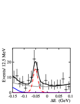
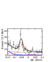
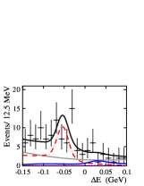
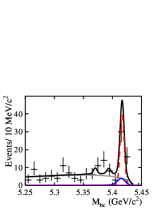
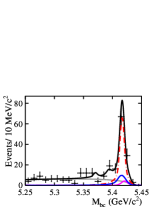
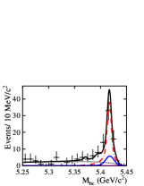
Figure 1: $M_{bc}$ and $\Delta E$ projections of the fit result. The columns correspond to $B_{s}^{0}\to D_{s}^{-}D_{s}^{+}$ (left), $B_{s}^{0}\to D_{s}^{*\pm}D_{s}^{*\mp}$ (middle), and $B_{s}^{0}\to D_{s}^{*-}D_{s}^{*+}$ (right). The red dashed curves show CR+WC signal, the blue and purple solid curves show CF, the grey solid curves show background, and the black solid curves show the total.

3 $\Delta\Gamma_{s}$ Estimation

In the heavy quark limit with $(m_{b}-2m_{c})\to 0$ and $N_{c}\to\infty$, the dominant contribution to the decay width comes from $B_{s}^{0}\to D_{s}^{(*)-}D_{s}^{(*)+}$ decays [5, 6]. Assuming negligible $CP$ violation, the branching fraction is related to $\Delta\Gamma_{s}$ as $\Delta\Gamma_{s}/\Gamma_{s}=2{\cal B}/(1-{\cal B})$. Inserting the total ${\cal B}$ from Table 1 gives

$$\frac{\Delta\Gamma_{s}}{\Gamma_{s}} = 0.090\pm 0.009\,\pm 0.023\,,$$ (1)

where the first error is statistical and the second is systematic. The precision of this result is similar to that of other recent measurements [7, 8] and consistent with theoretical predictions [10]. Two main uncertainties are the unknown $CP$-odd component in $B^{0}\to D^{*+}_{s}D^{*-}_{s}$ decay and the size of contributions from three-body final states. The former is estimated to be only $6\%$. However Ref. [9] calculates significant contribution from $B_{s}^{0}\to D_{s}^{(*)}D^{(*)}K^{(*)}$ decays. This calculation predicts $\Delta\Gamma_{s}/\Gamma_{s}$ from $D_{s}^{(*)+}D_{s}^{(*)-}$ alone to be $0.102\pm 0.030$, which agrees well with our result.

4 Polarization Measurement of $D_{s}^{*-}D_{s}^{*+}$

We have also made the first measurement of the longitudinal polarization fraction ($f_{L}$) of $D_{s}^{*-}D_{s}^{*+}$. We select events using the same criteria as before, however we use a narrower range of $M_{bc}$ and $\Delta E$ ($2.5\sigma$ in resolution) in order to minimize $B_{s}^{0}\to D_{s}^{*\pm}D_{s}^{*\mp}$ cross-feed. For these events we perform an unbinned maximum-likelihood fit to the helicity angles $\theta_{1}$ and $\theta_{2}$, which are the angles between the daughter $\gamma$ momentum and the opposite of the $B_{s}^{0}$ momentum in the $D^{*\pm}_{s}$ rest frame. The angular distribution is $\left(|A_{+}|^{2}+|A_{-}|^{2}\right)\left(\cos^{2}\theta_{1}+1\right)\left(\cos^{2}\theta_{2}+1\right)+|A_{0}|^{2}4\sin^{2}\theta_{1}\sin^{2}\theta_{2}$, where $|A_{+}|$, $|A_{-}|$, and $|A_{0}|$ are the helicity amplitudes. The fraction $f_{L}$ is given by $|A_{0}|^{2}/(|A_{0}|^{2}+|A_{+}|^{2}+|A_{-}|^{2})$. We measure

$$f_{L} = 0.06\,^{+0.18}_{-0.17}\,\pm 0.03\,,$$ (2)

where the first error is statistical and the second is systematic. The systematic errors are from signal PDF shapes ($+0.008,-0.010$), background PDF shape ($+0.007,-0.004$), fixed WC fractions ($+0.013,-0.015$), fixed background level ($\pm 0.022$), continuum suppression ($+0.011$), possible fit bias ($-0.011$), and MC efficiency due to statistics ($\pm 0.0004$). The helicity angle distributions and fit projections are shown in Fig. 2.

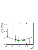
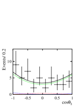
Figure 2: Helicity angle distributions and projections of the fit result. The green dashed (red dashed-dotted) curves show the transverse (longitudinal) components, the blue dotted curve shows background, and the black solid curve shows the total.

In summary, using the branching fractions of $B_{s}^{0}\to D_{s}^{(*)-}D_{s}^{(*)+}$ decays, we measured $\Delta\Gamma_{s}/\Gamma_{s}$ assuming no $CP$ violation, among other theoretical assumptions. We have also made the first measurement of the $B_{s}^{0}\to D_{s}^{*-}D_{s}^{*+}$ longitudinal polarization fraction.

References

• [1] S. Esen et al. (Belle Collab.), Phys. Rev. D (RC) (in press.); arXiv:1208.0323.
• [2] This result is obtained by Belle using 121.4 fb-1 of data and the method described in R. Louvot et al. (Belle Collab.), Phys. Rev. Lett. 102, 021801 (2009).
• [3] Charge-conjugate modes are implicitly included.
• [4] G. C. Fox and S. Wolfram, Phys. Rev. Lett. 41, 1581 (1978). The modified moments used in this paper are described in S. H. Lee et al. (Belle Collab.), Phys. Rev. Lett. 91, 261801 (2003).
• [5] M. A. Shifman and M. B. Voloshin, Sov. J. Nucl. Phys. 47, 511 (1988).
• [6] R. Aleksan et al., Phys. Lett. B 316, 567 (1993).
• [7] R. Aaij et al. (LHCb Collab.), Phys. Rev. Lett. 108, 101803 (2012).
• [8] T. Aaltonen et al. (CDF Collab.), Phys. Rev. Lett. 108, 201801 (2012).
• [9] C. -K. Chua, W. -S. Hou, and C. -H. Shen, Phys. Rev. D 84, 074037 (2011).
• [10] A. Lenz and U. Nierste, arXiv:1102.4274; J. High Energy Phys. 0706, 072 (2007).