Present Address: ]Departamento de Informática, Universidade Federal da Paraíba, CEP 58051-900 - João Pessoa, PB - Brazil.

Predictability and suppression of extreme events in a chaotic system

Abstract

f earthquakes, neuroscience, ecology, and even financial economics. In many complex systems, large events are believed to follow power-law, scale-free probability distributions, so that the extreme, catastrophic events are unpredictable. Here, we study coupled chaotic oscillators that display extreme events. The mechanism responsible for the rare, largest events makes them distinct and their distribution deviates from a power law. Based on this mechanism identification, we show that it is possible to forecast in real time an impending extreme event. Once forecasted, we also show that extreme events can be suppressed by applying tiny perturbations to the system.

Extreme events are increasingly attracting the attention of scientists and decision makers because of their impact on society Nott (2006); Comfort et al. (2010); Field et al. (2012); Barnosky et al. (2012), which is exacerbated by our increasing global interconnectivity. Examples of extreme events include financial crises, environmental and industrial accidents, epidemics and blackouts Schwab et al. (2013). From a scientific view point, extreme events are interesting because they often reveal underlying, often hidden, organizing principles Rundle et al. (1996); Sornette (2002); Albeverio et al. (2005). In turn, these organizing principles may enable forecasting and control of extreme events.

Some progress along these lines has emerged in studies of complex systems composed of many interacting entities. For example, it was found recently that complex systems with two or more stable states may undergo a bifurcation causing a transition between these states that is associated with an extreme event Scheffer et al. (2012); Biggs et al. (2009). Critical slowing down and/or increased variability of measureable system quantities near the bifurcation point open up the possibility of forecasting an impending event, as observed in laboratory-replicated populations of budding yeast Dai et al. (2012).

An open question is whether other underlying behaviors cause extreme events. One possible scenario is when the system varies in time and is organized by attracting sets in phase space. For example, a recent model of financial systems consisting of coupled, stochastically-driven, linear mappings Krawiecki et al. (2002) shows so-called bubbling behavior, where a bubble – an extreme event – corresponds to a large temporary excursion of the system state away from a nominal value. In this example, the event-size distribution follows a power law, having a “fat” tail that describes the significant likelihood of extreme events. One main characteristic of such distributions is that they are scale-free, which means that events of arbitrarily large sizes are caused by the same dynamical mechanisms governing the occurrence of small- and intermediate-size events, leading to an impossibility of forecasting Sornette (2009); Taleb (2007); Bak (1996); Embrechts et al. (2011); Knight (1921).

In contrast, the new concept of “dragon-kings” (DKs) emphasizes that the most extreme events often do not belong to a scale-free distribution Sornette (2009). DKs are outliers, which possess distinct formation mechanisms Sornette and Ouillon (2012). Such specific underlying mechanisms open the possibility that DKs can be forecasted, allowing for suppression and control. Here, we show DK-type statistics occurring in an electronic circuit that has an underlying time-varying dynamics identified to belong to a more general class of complex systems. Moreover, we identify the mechanism leading to the DKs and show that they can be forecasted in real time, and even suppressed by the application of tiny and occasional perturbations. The mechanism responsible for DKs in this specific system is attractor bubbling. As explained below, we argue that attractor bubbling is a generic behavior appearing in networks of coupled oscillators, and that DKs and extreme events are likely in these extended systems.

The large class of spatially extended coupled oscillator networks covers the physics of earthquakes Schmittbuhl et al. (1993), biological systems such as the collective phase synchronization in brain activity Gong et al. (2007), and even of financial systems made of interacting investors with threshold decisions and herding tendencies Takayasu et al. (1992). Many coupled-oscillator system models exhibiting chaos have invariant manifolds — subspaces of the entire phase space on which the system trajectory can reside. o another attractor, eventually followed by reinjection to the dominating attractor in many situations. In sum, attractor bubbling associated with riddled basins of attraction is a generic mechanism for DKs, which we conjecture apply to a large class of spatially extended deterministic and stochastic nonlinear systems. Such manifolds commonly occur in models where identical chaotic systems are coupled and synchronize. Furthermore, when invariant manifolds contain chaotic orbits, they can lead to attractor bubbling (as well as riddled basins and on-off intermittency) Ott (2002); Sommerer and Ott (1993); Mosekilde et al. (2002); Ashwin et al. (1994). Attractor bubbling is a situation where the system trajectory irregularly and briefly leaves the vicinity of an invariant manifold containing a chaotic attractor as a result of an occasional noise-induced jump into a region where orbits are locally repelled from the invariant manifold. The system state then follows an orbit that moves away from the invariant manifold, but eventually returns to the attractor. These excursions of the system state to phase space regions far from the invariant manifold are our extreme events.

To highlight the connection between attractor bubbling and DKs we study two nearly identical unidirectionally-coupled chaotic electronic circuits in a master (mnemonic $M$) and slave ($S$) configuration. The state of each circuit is described by a three-dimensional (3D) vector whose components are related to the two voltages and the current of each circuit (see Fig. S1 ). The temporal evolution of the state vectors is governed by the differential equations

$$\dot{\mathbf{x}}_{M} =\mathbf{F}\left[\mathbf{x}_{M}\right],$$ (1)

$$\dot{\mathbf{x}}_{S} =\mathbf{F}\left[\mathbf{x}_{S}\right]+c\mathbf{K}\left(\mathbf{x}_{M}-\mathbf{x}_{s}\right),$$ (2)

where the dot over a variable means differentiation with respect to time, $\mathbf{F}\left[\mathbf{x}\right]$ is the flow for each subsystem, $c$ controls the interaction strength between the subsystems, and $\mathbf{K}$ is the coupling matrix. In general, the coupled system resides in a 6D phase space spanned by $\left(\mathbf{x}_{M},\mathbf{x}_{S}\right)$. However, for appropriate values of $c$ and $\mathbf{K}$, the coupled oscillators synchronize their behavior Sommerer and Ott (1993), which corresponds to $\mathbf{x}_{M}=\mathbf{x}_{S}$. Hence, the coupled-system trajectory resides in a restricted 3D subspace (on an invariant manifold). In this case, it is insightful to introduce new 3D state vectors that describe the behavior on the invariant manifold $\mathbf{x}_{\parallel}=\left(\mathbf{x}_{M}+\mathbf{x}_{S}\right)/2$ and transverse to the manifold $\mathbf{x}_{\perp}=\left(\mathbf{x}_{M}-\mathbf{x}_{S}\right)/2$. Synchronization corresponds to $\mathbf{x}_{\perp}=0$ and $\mathbf{x}_{\parallel}=\mathbf{x}_{M}$, and the basin of attraction associated with the synchronized state is riddled.

Here we study a pair of electronic circuits for which the equations (1) and (2) take the form

$$\dot{V}_{1j} =\frac{V_{1j}}{R_{1}}-g\left[V_{1j}-V_{2j}\right],$$ (3)

$$\dot{V}_{2j} =g\left[V_{1j}-V_{2j}\right]-I_{j}+\delta_{S,j}c\left(V_{2M}-V_{2S}\right),$$ (4)

$$\dot{I}_{j} =V_{2j}-R_{4}I_{j},$$ (5)

for $j=M,S$, respectively, $\delta_{S,j}$ is the Kronecker delta ($1$ if $j=S$ and $0$ if $j=M$), and

$$g\left[V\right]=\frac{V}{R_{2}}+I_{r}\left(\exp(\alpha_{f}V)-\exp(-\alpha_{r}V)\right).$$ (6)

The values of the parameters and other details are given in Note (1); Gauthier and Bienfang (1996). Equations (3-5) correspond to Eqs. (1-2) with $\mathbf{x}_{j}=(V_{1j},V_{2j},I_{j})^{T}$, where $\mathbf{x}^{T}$ denotes the transpose of vector $\mathbf{x}$, and the coupling matrix $\mathbf{K}$ is such that the matrix entry $K_{m,n}$ is $1$ for $m=n=2$ and $0$ otherwise.

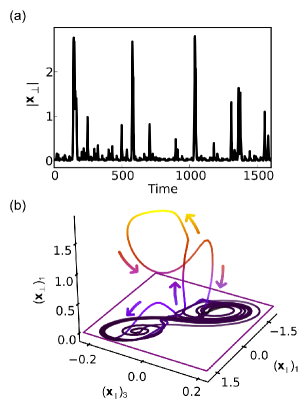
Figure 1: (color online). Experimental observation of attractor bubbling in coupled chaotic oscillators. (a) Typically observed temporal evolution of $\lvert\mathbf{x}_{\perp}\rvert$ for $c$ = 4.4. Time is measured in dimensionless units corresponding to the characteristic time in the circuit (see Supplemental Material). (b) Illustration of the system trajectory in the vicinity of a bubbling event. The 6D phase space is projected onto a 3D space, where the subscript on the axis label indicates the $i^{\mathrm{th}}$ component of the corresponding vector. The arrows indicate the direction of the flow and the colors indicate the height on the $\left(\mathbf{x}_{\perp}\right)_{1}$ direction.

As discussed above, attractor bubbling occurs when noise is present (e.g., thermal noise in the electronic components), when there is a slight parameter mismatch between the oscillators (the flows of each circuit are slightly different), or when both effects are present, which is the most likely situation in an experiment. Bubbling is indicated by long excursions of high-quality synchronization ($\mathbf{x}_{\perp}$ close to the noise level) interspersed by brief desynchronization events where $\mathbf{x}_{\parallel}$ takes on a large value — an extreme event — as shown in Fig. 1(a). We illustrate the trajectory of a typical bubbling event in Fig. 1(b), which is a projection of the 6D phase space onto a 3D space containing components of the invariant manifold and of the transverse manifold. It is seen that the trajectory remains for most of the time on the invariant manifold $\mathbf{x}_{\parallel}$, but undergoes a large excursion away fro m the invariant manifold during the bubbling event. Due to the nonlinear folding of the flow, the trajectory is reinjected to the invariant manifold after the bubble.

To reveal the existence of DKs, we collect a long time series of values of $\lvert\mathbf{x}_{\perp}\rvert$, use a peak-detecting algorithm to identify the bubbling events, and create a probability density function (PDF) for the event-sizes $\lvert\mathbf{x}_{\perp}\rvert_{n}$, defined as the largest peak-value of $\lvert\mathbf{x}_{\perp}\rvert$ within a burst. The length of the time series is large enough that the observed PDFs have reached statistical convergence and are stationary, in the sense that their shape does not change appreciably with the addition of new samples. The resulting distribution is shown in Fig. 2, where the event-sizes follow approximately a power-law distribution (straight line in log-log scale) for small to moderately large sizes ($0.04<\lvert\mathbf{x}_{\perp}\rvert_{n}<1.8$) with exponent $-2.0\pm 0.1$. We apply a Kolmogorov-Smirnov (K-S) statistical hypothesis test to check that the distribution of event sizes follows a power law in this interval. The hypothesis of a truncated power-law is rejected for the raw data because there are small but statistically significant deviations from a straight line decorating the distribution. The hypothesis of a truncated power-law is accepted with the same value of the exponent obtained in the fit if we apply a decimation of correlated data by resampling the raw data Note (1). This empirical observation is substantiated by a theoretical analysis based on the statistics of the perturbations affecting trajectories near the fixed point at the origin Note (1). The analysis predicts that the exponent is $-2$ to leading order. Moreover, the observed desynchronization events can be rationalized as being associated with the structure of the repeller around the origin, consistent with current theory of attractor bubbling.

A substantial and significant peak in the distribution and subsequent cut-off that deviates from the power law is observed for the extremely large events ($\lvert\mathbf{x}_{\perp}\rvert_{n}>2.4$), which we associate with dragon-kings. Interestingly, the probability mass contained in the large peak associated to the DKs is approximately equal to the integral of the PDF that would result if the power law extended to infinity. This fact suggests that the DKs are events that would belong to a power-law distribution but had their size limited by some saturation mechanism that effectively determines a maximum size for the events in the system. The K-S hypothesis test verifies that this large peak in the PDF deviates significantly from a pure power-law, as expected from theory, using either the raw data or the decimated data Note (1). Hence, the theory developed assuming linearization near the fixed point captures the essence of the bubbling (power law with exponent $-2$ and dragon-king peak of the PDF), and only fails to explain the tiny structures decorating the distribution.

Figure 2: Appearance of dragon-kings. Bubble event-size probability density function (PDF) for $c$ = 4.4. The dashed line is a fit to a power law.

As discussed some time ago Ashwin et al. (1994); Heagy et al. (1995), a bubbling event is initiated by “hot spots” within the chaotic attractor that resides on the invariant manifold. The attractor is composed of a large (likely infinite) number of unstable sets, such as unstable fixed points, unstable periodic orbits, etc. Ott (2002). Each of these sets has an associated local transverse Lyapunov exponent Heagy et al. (1995), which describes the tendency of a trajectory to be attracted to or repelled from the invariant manifold when it is in a neighborhood of the set. A system with attractor bubbling necessarily has a distribution of local Lyapunov exponents (see Fig. S2 Note (1)), where at least some are repelling (value greater than zero), even though the value of the weighted average is negative (attracting). The repelling sets correspond to the hot spots on the invariant manifold.

For the coupled oscillators studied here, it was found previously that one set in particular — the unstable, saddle-type fixed point at $\mathbf{x}_{\parallel}=0$ — is exceedingly transversely unstable and is the underlying originator of the largest bubbles Gauthier and Bienfang (1996); Venkataramani et al. (1996). That is, there is a very high likelihood that a bubble will occur whenever $\mathbf{x}_{\parallel}$ resides in a neighborhood of the origin for some time, and the largest events (the DKs) occur when the residence time is long and the approach is close. The large bubble event shown in Fig. 1(b) clearly originates near $\mathbf{x}_{\parallel}=0$. This observation is at the heart of the theoretical approximation for the distribution of event sizes, where we approximate the dynamics of perturbations by linearization of the equations of motion (Eqs. (3) to (5), for $j=M,S$) near the fixed point.

The influence of the fixed point in the dynamics also allows us to predict the occurrence of a large event by real-time observation of $\mathbf{x}_{M}$, which is equal to $\mathbf{x}_{\parallel}$ when the subsystems are synchronized, and finding the times when it approaches the origin. Figure 3 shows the temporal evolution of $\lvert\mathbf{x}_{M}\rvert$ and $\lvert\mathbf{x}_{\perp}\rvert$, where it is seen that $\lvert\mathbf{x}_{M}\rvert$ undergoes a sustained drop and remains below an empirically determined threshold value $\lvert\mathbf{x}_{M}\rvert_{\mathrm{th}}$ preceding a large bubble (spike in $\lvert\mathbf{x}_{\perp}\rvert$), where the forecasting time is denoted by $t_{p}$. A smaller threshold is associated with a larger event size and hence it can be adjusted to isolate the DKs. This description and ensuing results are confirmed by numerical integration of Eqs. (3-5), which shows excellent agreement with the experimental observations Note (1) and demonstrates that it is possible to forecast DKs in this relatively low-dimensional complex system.

Figure 3: Forecasting dragon-kings. Temporal evolution of the trajectory projected onto the invariant manifold ($\lvert\mathbf{x}_{M}\rvert$) and the transverse space ($\lvert\mathbf{x}_{\perp}\rvert$) during attractor bubbling ($c$ = 4.4). The largest, extreme event, which is part of the dragon-king distribution, is preceded by a long excursion of $\lvert\mathbf{x}_{M}\rvert$ below a threshold of $\lvert\mathbf{x}_{M}\rvert_{\mathrm{th}}=0.50$ whose value is determined empirically by minimizing the number of false predictions.

With this scheme to forecast DKs, we design a feedback method to suppress them based on occasional proportional feedback of tiny perturbations to the slave oscillator when $\lvert\mathbf{x}_{M}\rvert<\lvert\mathbf{x}_{M}\rvert_{\mathrm{th}}$ Newell et al. (1994). In the presence of feedback, the temporal evolution of the slave oscillator (Eq. (2)) is modified to read

$$\dot{\mathbf{x}}_{S}= \mathbf{F}\left[\mathbf{x}_{S}\right]+c\mathbf{K}\left(\mathbf{x}_{M}-\mathbf{x}_{s}\right)+$$ (7)

$$\left[1-\theta\left(\lvert\mathbf{x}_{M}\rvert-\lvert\mathbf{x}_{M}\rvert_{\mathrm{th}}\right)\right]c_{DK}\mathbf{K}_{DK}\left(\mathbf{x}_{M}-\mathbf{x}_{s}\right),$$

where $\theta$ is the Heaviside step function, and $c_{DK}$ ($\mathbf{K}_{DK}$) is the feedback strength (coupling matrix) used to suppress DKs. For the purpose of illustration, we assume that it is expensive or not convenient to keep this additional feedback coupling on all the time and thus it is only active for a brief interval when necessary.

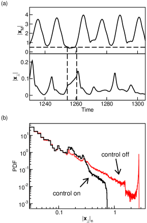
Figure 4: (color online). Slaying dragon-kings. (a) Temporal evolution of the trajectory projected onto the invariant manifold ($\lvert\mathbf{x}_{M}\rvert$) and the transverse space ($\lvert\mathbf{x}_{\perp}\rvert$) during suppressed attractor bubbling. When $\lvert\mathbf{x}_{M}\rvert$ is below $\lvert\mathbf{x}_{M}\rvert_{\mathrm{th}}=0.50$ (the horizontal dashed line) the occasional feedback is activated, reducing the height of a bubble (in the time interval between the two vertical dashed lines) that would grow large otherwise. (b) Probability density function for event-size $\lvert\mathbf{x}_{\perp}\rvert_{n}$ in the presence (black) and absence (red online) of occasional proportional feedback. Here $c$ = 4.4, $c_{DK}$ = 0.55, $\mathbf{K}_{ij}=1$ for $i=j=2$ and $0$ otherwise, and $\left(\mathbf{K}_{DK}\right)_{ij}=1$ for $i=j=1$ and $0$ otherwise. A more detailed comparison between experiment and theory is presented in Note (1).

Figure 4(a) shows the temporal evolution of the system in the presence of occasional feedback. When $\lvert\mathbf{x}_{M}\rvert>\lvert\mathbf{x}_{M}\rvert_{\mathrm{th}}$, no feedback is applied and the small bubbling events are allowed to proceed. On the other hand, when $\lvert\mathbf{x}_{M}\rvert<\lvert\mathbf{x}_{M}\rvert_{\mathrm{th}}$, feedback perturbations are applied that are only 3% of the system size (defined as the maximum value of $\lvert\mathbf{x}_{M}\rvert\sim 4$). Such small perturbation only causes a small change in $\mathbf{x}_{S}$, yet it has a dramatic change in $\mathbf{x}_{\perp}$: the large bubble is suppressed. Over a long time scale, feedback is only applied 1.5% of the time, consistent with the frequency and duration of extreme events. Thus, the total perturbation size averaged over the whole time, including the intervals when the perturbation is not active, corresponds to 0.05% of the system size. As a result of this occasional feedback, we observe that the largest events, i ncluding the DKs, are entirely suppressed, as shown in the probability density function for $\lvert\mathbf{x}_{\perp}\rvert$ in Fig. 4(b). It is seen that the small- to intermediate-size bubbles are unaffected; only the events that would have a large size in the absence of control are suppressed.

Our work addresses several important questions regarding complex systems. We answer affirmatively and conclusively that: 1) a particular simple, but nontrivial system displays DKs whose event-size distribution deviates significantly upward from a power law in the tail; 2) DKs can be predicted; and 3) this predictability can be used to occasionally and efficiently activate countermeasures that suppress or mitigate the effects of DKs. An important and immediate open question is whether it is possible to easily identify the unstable sets that are primarily responsible for causing DKs in the wide variety of complex systems that are already known to have attractor bubbling or in systems that may display bubbling but it is not yet appreciated that the behavior is of this type. While a specific method that is valid in all cases is unlikely to exist, the particular example studied here demonstrates that, with some understanding of the burst mechanism, large DK-type events may potentially be avoidable by devising small, well-chosen system perturbations. Key to addressing this problem is the development of new tools for analyzing models of complex systems or for time series analysis of natural systems that can identify burst mechanisms. We suggest that the use of this knowledge to devise appropriate control strategies is a worthy pursuit given the increasing appearance of extreme events and their impact on society.