Sampling and reconstruction of solutions to the Helmholtz equation

Abstract

We consider the inverse problem of reconstructing general solutions to the Helmholtz equation on some domain $\Omega$ from their values at scattered points $x_{1},\dots,x_{n}\subset\Omega$. This problem typically arises when sampling acoustic fields with $n$ microphones for the purpose of reconstructing this field over a region of interest $\Omega$ contained in a larger domain $D$ in which the acoustic field propagates. In many applied settings, the shape of $D$ and the boundary conditions on its border are unknown. Our reconstruction method is based on the approximation of a general solution $u$ by linear combinations of Fourier-Bessel functions or plane waves. We analyze the convergence of the least-squares estimates to $u$ using these families of functions based on the samples $(u(x_{i}))_{i=1,\dots,n}$. Our analysis describes the amount of regularization needed to guarantee the convergence of the least squares estimate towards $u$, in terms of a condition that depends on the dimension of the approximation subspace, the sample size $n$ and the distribution of the samples. It reveals the advantage of using non-uniform distributions that have more points on the boundary of $\Omega$. Numerical illustrations show that our approach compares favorably with reconstruction methods using other basis functions, and other types of regularization.
Key words and phrases : Helmholtz equation, interpolation, least squares, regularization
MSC2000: 74J25,35J05,94A20

1 Introduction

A common inverse problem in acoustics is to obtain a precise approximation of the soundfield over a spatial domain $\Omega$ of interest, using the smallest possible number of pointwise measurements, e.g. as provided by microphones. For instance, one may wish to measure the complex radiation pattern of an extended source (source identification problem), to localize a number of point sources within a spatial domain (source localization problem), or to optimize the output of a sound reproduction system over a large control area, to name only a few applications. In practice, the main difficulty that one is usually faced with is how to handle reverberation: the reverberant field might well be of a magnitude comparable to the direct sound, and it depends in a non-trivial way on both the geometry of the domain $D$ where the acoustic field is defined and the type of boundary conditions on $\partial D$ (with Dirichlet or Neumann as ideal cases, but more likely in engineering problems with a frequency-dependent mixed behavior).

The goal of this paper is to study the accuracy that can be achieved when approximating the acoustic field over the domain $\Omega\subset D$, based on a set of point measurements, without precise knowledge on the geometry of $D$ and boundary conditions on $\partial D$. A general setting is the following: the soundfield $p(x,t)$ is measured at microphones located at positions $x_{1},\dots,x_{n}\in\Omega$, and over a (discretized) time interval $[0,T]$. After application of the (discrete) Fourier transform ${\mathcal{F}}$ in the time variable, and considering a given frequency $\omega$, the function

$$u(x):={\mathcal{F}}p(x,\omega)$$

is a solution on $D$ to the Helmholtz equation

$$\Delta u+\lambda^{2}u=0,$$ (1)

where $\lambda=\omega/c$, with $c$ denoting the wave velocity, and where the boundary conditions are unknown to us.

Depending on the applications, the geometry of the domain $\Omega$ may either be $2$-D (membranes) or $3$-D (rooms). Our problem therefore amounts to reconstructing, on some domain $\Omega\subset{\mathbf{R}}^{2}\mbox{ or }{\mathbf{R}}^{3}$, a general solution to the Helmholtz equation (1) from its sampling at points $x_{1},\dots,x_{n}\in\Omega$. These samples may be measured exactly or up to some additive noise. We denote by

$$y_{l}=u(x_{l})+\eta_{l},\quad\quad l=1,\dots,n,$$ (2)

these samples, where $\eta_{l}$ represent the additive noise.

Reconstruction from scattered points is a widely studied topic, and a variety of methods have been proposed and analyzed. Many existing methods can be viewed as reconstructing some form of approximation to the unknown function $u$ by simpler functions such as splines, partial Fourier sums or radial basis functions. The success of these methods therefore relies in good part on the quality of the approximation of $u$ by such simpler functions, which is typically governed by the smoothness of $u$.

In our present setting, the fact that $u$ obeys the Helmholtz equation, may be used in addition to its smoothness in order to guarantee the accuracy of certain approximation schemes, which are well adapted to such solutions.

The fact that the function to be measured is solution to the Helmholtz equation can be used in various ways:

• As can be seen on Fig. 1, the spectrum of a solution to the equation (in 2D) is concentrated on an annulus. This annulus can be enclosed in a square, or an hexagon, allowing reconstruction of the function from its values on a square or hexagonal lattice, using the Shannon-Nyquist sampling theorem.

• The recent field of compressed sensing suggests to interpret this property as the sparsity of the function in a dictionary of Fourier-modes, and to reconstruct the function from a random sampling of the function on the domain of interest.

• The function can be reconstructed from its value on the border on the domain, as well as the value of its normal derivative, using the Green formula:

  $$u(x)=\int_{\partial\Omega}u(y)\frac{\partial G}{\partial n}(y,x)-G(y,x)\frac{\partial u}{\partial n}(y)ds.$$

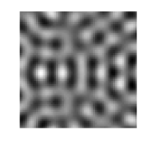
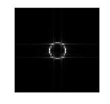
Figure 1: A solution to the Helmholtz equation in 2D and its 2D Discrete Fourier Transform

The last method is however not relevant for our setting, in which we are allowed to measure the function but not its derivatives. The two first methods will be compared with the method we propose, based on the expansion of solutions to the Helmholtz equation on particular families of function and least-squares approximations.

We introduce the Fourier-Bessel functions

$$b_{\lambda,j}(x):=e^{ij\theta}J_{j}(\lambda r)$$ (3)

where $(r,\theta)$ are the polar coordinates of $x$ and $J_{j}$ is the $j$-th Bessel function of the first kind. $b_{\lambda,j}$ is solution to the Helmholtz equation (1) over ${\mathbf{R}}^{2}$ if and only if its parameter $\lambda$ is the same as in (1). Denoting $V_{\lambda}$ the set of the solutions of (1), it is known [6] that

$$V_{\lambda}=\overline{{\rm span}\{b_{\lambda,j}\}}^{L^{2}(\Omega)},$$ (4)

and that the solutions of (1) can be approximated by elements of the subspaces $V^{b}_{m}={\rm span}\{b_{\lambda,j},-L\leq j\leq L\}$ as $m=2L+1$ grows.

An alternative approximation scheme uses plane waves defined by

$$e_{{\mathbf{k}}}(x):=e^{i{\mathbf{k}}\cdot x}$$ (5)

which are solutions of (1) if and only if $|{\mathbf{k}}|=\lambda$. The spaces $V^{e}_{m}$, spanned by the particular plane waves

$$e_{j}:=e_{{\mathbf{k}}_{j}},\;\;{\mathbf{k}}_{j}:=\lambda\left(\cos\left(\frac{2j\pi}{m}\right),\sin\left(\frac{2j\pi}{m}\right)\right),\;\;j=-L,\dots,L,$$ (6)

can also be used to approximate solutions of (1) as $m$ grows [6].

The most widely used approach to approximate $u$ in a finite dimensional space $V_{m}$, from its data at points $x_{1},\dots,x_{n}$, is the least squares method, namely with $m\leq n$ solving the minimization problem

$$\pi=\operatorname*{argmin}_{v\in V_{m}}\frac{1}{n}\sum_{i=1}^{n}|y_{i}-v(x_{i})|^{2}.$$ (7)

The effectiveness of the least squares approximation is governed by a certain trade-off in the choice of the dimension $m$ of the approximation:

• A small value of $m$ leads to a highly regularized reconstruction of $u$, which is usually robust but has poor accuracy.

• A large value of $m$ may lead to unstable and therefore inaccurate reconstructions although the space $V_{m}$ contains finer approximants to $u$.

Let us observe that regularization is relevant even in a noiseless context where the function is measured exactly: for example choosing $m=n$ corresponds to searching for an exact interpolation of the data which may be very unstable and inaccurate, a phenomenon similar to the Runge phenomenon in polynomial approximation.

In this paper, we discuss the amount of regularization which is needed when applying the least squares method using the finite dimensional subspaces $V^{b}_{m}$ and $V^{e}_{m}$ extracted from $V_{\lambda}$. With such discretizations, the distribution of the sampling points $x_{1},\dots,x_{n}$ has an influence on the above described trade-off. Our main theoretical result, established in the case of a disc, shows that higher values of $m$, leading therefore to better accuracy, can be used if the $x_{i}$ are not uniformly distributed on $\Omega$ in the sense that a fixed fraction of these points are located on the boundary $\partial\Omega$. This result is confirmed by numerical experiments.

The rest of this paper is organized as follow: we give a brief account in §2 on approximation of solutions to (1) by Fourier-Bessel functions and plane waves which relies on Vekua’s theory, and in §3 on general results on the stability and accuracy of least-squares approximations recently established in [4]. We then study in §4 the spaces $V^{e}_{m}$ and $V^{b}_{m}$ in more detail, in the particular case where $\Omega$ is a disc, and use the above mentioned results to compare least-squares approximations on these spaces based on different sampling strategies. We also give similar results for the case of the 3D ball. In §5, we present numerical tests that illustrate the validity of this comparison. We also show that our approach compares favorably with reconstructions based on other approximation schemes such as partial Fourier sums (that do not exploit the fact that $u$ is a solution to (1)) and to other form of regularizations such as weighted Basis Pursuit. In §6, we discuss further issues, namely determination of the model order via cross-validation, and the influence of the sampling distribution in the treatment of more general domains.

2 Approximation by Fourier-Bessel functions and plane waves

Results on the approximation of solutions to (1) by Fourier-Bessel functions and plane waves given in [6] are based on the theory developed in the 1950’s by Vekua [14]. This theory generalizes approximation results for holomorphic functions, viewed as solutions of $\Delta u=0$, to solutions of more general elliptic partial differential equations, by means of appropriate operators that link the two types of solutions.

In the case of the Helmholtz equation on a domain $\Omega$, that is star-shaped with respect to a point which is fixed as the origin $0$, these operators (in their version mapping harmonic functions to solutions to (1)) have the explicit expression

$${\mathcal{V}}_{1}\phi(x)=\phi(x)-\frac{\lambda|x|}{2}\int_{0}^{1}\frac{1}{\sqrt{1-t}}J_{1}(\lambda|x|\sqrt{1-t})\phi(tx)dt,$$ (8)

and

$${\mathcal{V}}_{2}\phi(x)=\phi(x)-\frac{\lambda|x|}{2}\int_{0}^{1}\frac{1}{\sqrt{t(1-t})}I_{1}(\lambda|x|\sqrt{1-t})\phi(tx)dt,$$ (9)

where $|x|$ stands for the euclidean norm of $x$, $J_{1}$ is the Bessel function of the first kind of order $1$ and $I_{1}$ the modified Bessel function of the first kind of order $1$, see [7] for more details. These operators have important properties:

• They are linear.

• ${\mathcal{V}}_{1}$ maps harmonic functions to solutions of the Helmholtz equation, and ${\mathcal{V}}_{2}$ does the converse.

• When restricted to harmonic functions or solutions to the Helmholtz equation, they are continuous in the Sobolev $H^{k}$ norms for all $k\geq 0$.

• They are inverse to each other on these spaces.

As a consequence, any approximation method for harmonic functions can be translated as an approximation method for solutions of the Helmholtz equation. In particular, approximation of harmonic functions by harmonic polynomials of degree $m$ translates as approximation of solution of the Helmholtz equation by the so-called generalized harmonic polynomials $m$ which are their image by $V_{1}$. The generalized harmonic polynomials of degree $m$ can be expressed as linear combinations of the Fourier-Bessel functions (3), leading therefore to results for the approximation of solutions to (1) by elements of $V_{m}^{b}$ in Sobolev norms. More precisely, the following result can be obtained when the domain $\Omega$ is convex, see theorem 3.2 of [6]

$$\min_{v\in V^{b}_{m}}\|u-v\|_{H^{k}}\leq C\left(\frac{\log m}{m}\right)^{p-k}\|u\|_{H^{p}},$$ (10)

where the constant $C$ depends on $p$, $k$, $\lambda$ and the geometry of $\Omega$. This results still holds for more general, star-shaped convex domains, with a slower convergence.

Plane waves and Bessel functions are related by the Jacobi-Anger identity

$$e_{\mathbf{k}_{\phi}}=\sum_{m\in{\mathbf{Z}}}i^{m}J_{m}(\lambda r)e^{im(\theta-\phi)}.$$ (11)

where ${\mathbf{k}}_{\phi}:=\lambda(\cos(\phi),\sin(\phi))$, and its converse, the Bessel integral

$$J_{n}(\lambda r)e^{in\theta}=\frac{1}{2\pi i^{n}}\int_{-\pi}^{\pi}e_{{\mathbf{k}}_{\phi}}e^{in\phi}d\phi,$$ (12)

Approximating the integral in (12) by a discrete sum, by uniformly sampling the wave vectors ${\mathbf{k}}_{\phi}$ on the circle of diameter $\lambda$, leads to approximations of solutions to (1) by linear combinations of the $2m+1$ plane waves $e_{\mathbf{k}_{j}}$, that is, by elements of $V_{m}^{e}$. It is also known (see theorem 5.2 of [6]) that such approximations have the same convergence properties, e.g., for a convex domain,

$$\min_{v\in V^{b}_{e}}\|u-v\|_{H^{k}}\leq C\left(\frac{\log m}{m}\right)^{p-k}\|u\|_{H^{p}}.$$ (13)

3 Least-square approximations

The results of the previous section quantify how a general solution $u$ to the Helmholtz equation can be approximated by functions from spaces $V^{e}_{m}$ or $V^{b}_{m}$. We are now interested in understanding the quality of approximations from these spaces built by the least squares methods based on scattered data $(x_{l},y_{l})_{l=1,\dots,n}$. In particular, we want to understand the trade-off between the dimension $m$ and the number of samples $n$. Ideally we would like to choose $m$ large in order to benefit of the approximation properties (10) and (13), however not too large so that stability of the least-square method is ensured. We are also interested in understanding how the spatial distribution of the sample $x_{l}$ influences this trade-off.

This problem was recently studied in [4], in a general setting where the $x_{l}$ are independently drawn according to a given probability measure $\nu$ defined on $\Omega$. This measure therefore reflects the spatial distribution of the samples. For example, the uniform measure

$$d\nu:=|\Omega|^{-1}dx,$$ (14)

tends to generate uniformly spaced samples. In order to present the general result of [4], we assume that $(V_{m})_{m\geq 1}$ is an arbitrary sequence of finite dimensional spaces of functions defined on $\Omega$ with $\dim(V_{m})=m$.

We introduce the $L^{2}$ norm with respect to the measure $\nu$

$$\|v\|:=\left(\int_{\Omega}|v|^{2}d\nu\right)^{1/2},$$ (15)

and we define the best approximation error for a function $u$ in this norm as

$$\sigma_{m}(u):=\min_{v\in V_{m}}\|u-v\|.$$ (16)

Note that, in the noiseless case, the least squares method amounts to computing the best approximation of $u$ onto $V_{m}$ with respect to the norm

$$\|v\|_{n}:=\left(\frac{1}{n}\sum|v(x_{l})|^{2}\right)^{1/2}.$$ (17)

This norm can be viewed as an approximation of the norm $\|v\|$ based on the draw, and it is therefore natural to compare the error $\|u-\pi\|$ where $\pi$ is computed by (7) with $\sigma_{m}(u)$. We give below a criterion that describes under which condition on $m$ these two quantities are of comparable size.

Here, we assume that $(L_{1},\dots,L_{m})$ is a basis of $V_{m}$ which is orthonormal in $L^{2}(\Omega,\nu)$. We define the quantity

$$K(m)=K(V_{m},\nu):=\max_{x\in\Omega}\sum_{j=1}^{m}|L_{j}(x)|^{2},$$ (18)

which depends both on $V_{m}$ and on the chosen measure $\nu$, but not on the choice of the orthonormal basis since it is invariant by rotation.

We also assume that an a-priori bound $\|u\|_{L^{\infty}}\leq M$ is known on the function $u$. We can therefore only improve the least squares estimate by defining

$$\tilde{u}:=T_{M}(\pi),$$ (19)

where $T_{M}(t):={\rm sign}(t)\min\{|t|,M\}$ and $\pi$ is given by (7). The following result was established in [4], in the case of noiseless data, i.e. $\eta_{l}=0$ in (2).

Theorem 3.1

Let $r>0$ be arbitrary but fixed and let $\kappa:=\frac{1-\log 2}{2+2r}$. If $m$ is such that

$$K(m)\leq\kappa\frac{n}{\log n},$$ (20)

then, the expectation of the reconstruction error is bounded:

$$E(\|u-\tilde{u}\|^{2})\leq(1+{\varepsilon}(n))\sigma_{m}(u)^{2}+8M^{2}n^{-r},$$ (21)

where ${\varepsilon}(n):=\frac{4\kappa}{\log n}\to 0$ as $n\to+\infty$.

It is also established in [4] that the condition (20) ensures the numerical stability of the least-square method, with probability larger than $1-2n^{-r}$. These results suggest to set the regularization level by picking the largest value of $m^{*}=m^{*}(n)$ such that (20) holds. The dependence of $m^{*}(n)$ with $n$ is obviously related to that of $K(m)$ with $m$. In particular, slower growth of $K(m)$ with $m$ implies faster growth of $m^{*}(n)$ and therefore faster convergence of the least squares approximation. Notice that we always have

$$K(m)\geq\int_{\Omega}\sum_{j=1}^{m}|L_{j}|^{2}d\nu=m.$$ (22)

In the next section, we evaluate $K(V^{e}_{m},\nu)$ and $K(V^{e}_{b},\nu)$ in the case where $\Omega$ is a disk, for various choices of the measure $\nu$.

4 Stability of the reconstruction on a disc and in a ball

As mentioned in the previous section, the quantity $K(m)$ depends both on the space $V_{m}$ and the measure $\nu$ that reflects the sampling strategy. Here we study the case where $V_{m}$ is either one of the spaces of plane waves $V^{e}_{m}$ or of Fourier-Bessel functions $V^{b}_{m}$ defined in the introduction, for $m=2L+1$. We consider two sampling strategies. The first one uses the uniform probability distribution

$$\nu_{0}:=\frac{dx}{|\Omega|},$$ (23)

and the second one combines uniform sampling on the domain and on its boundary, with proportion $0<\alpha<1$, according to the probability distribution

$$\nu_{\alpha}:=(1-\alpha)\frac{dx}{|\Omega|}+\alpha\frac{d\sigma}{|\partial\Omega|}.$$ (24)

Examples of such densities are pictured on figure 2. The norm computed using these densities is simply denoted $\|\cdot\|$.

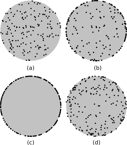
Figure 2: Examples of sampling distributions on the disc: (a) $\nu_{0}$, (b) $\nu_{1/2}$, (c) $\nu_{1}$ (d) $\nu^{\prime}$, defined and used in section 5.

This particular choice of probability distribution makes it possible to control the $L_{2}(\Omega)$-norm of the error. Indeed, theorem 3.1 control the reconstruction error in the norm defined by $\nu_{\alpha}$, which itself can bound the $L_{2}(\Omega)$-norm of the error as

$$\|u\|_{L_{2}(\Omega)}\leq\frac{1}{1-\alpha}\|u\|.$$ (25)

In order to obtain explicit results, we focus on the simple case where $\Omega$ is a disk. Without loss of generality, we fix

$$\Omega:=\{x\in{\mathbf{R}}^{2}\;:\;|x|\leq 1\}.$$ (26)

4.1 Fourier-Bessel approximation on the disc

Fourier-Bessel functions are orthogonal on the disk with respect to any rotation-invariant measure, because of their angular dependence in $e^{in\theta}$. This allows a simple computation of the quantity $K(m)$ for the space $V_{m}^{b}$, leading to the following result.

Theorem 4.1

For the space $V_{m}^{b}$ and the measure $\nu_{\alpha}$ on the unit disk $\Omega$, one has for sufficiently large $m$

$$K(m)\geq c_{0}+c_{1}m^{2},$$ (27)

when $\alpha=0$ (that is, for the uniform measure), for any $c_{1}<1/16$, and where $c_{0}$ depends on $c_{1}$ and $\lambda$, and

$$K(m)\leq C+\frac{m}{\alpha},$$ (28)

when $\alpha>0$, where $C$ depends on $\lambda$ and $\alpha$.

This result indicates that using an order $m$ for the approximation necessitates a number of samples $n$ that scales at least quadratically with $m$ when sampling uniformly in the disk. Using a proportion $\alpha$ of samples on the border makes $K(m)$ linear with respect to $n$. The best behavior possible for $K$ (i.e. $K(m)=m$) can be approached when $\alpha$ approaches 1. However in that case, the constant $C$ may grow, and the bound (25) becomes less efficient. This would make the use of a large proportion of samples on the border relevant only for very large numbers of samples.

Note finally that in the case $\alpha=1$, Eq. (25) cannot be used to control the $L_{2}(\Omega)$-norm of the error, allowing arbitrary large errors with any number of samples. For instance, when $\lambda$ is an eigenfrequency of the disk with Dirichlet boundary conditions, the associated eigenmode (a Fourier-Bessel function) cannot be recovered as its samples on the border are identically zero.

Proof: Since the Fourier-Bessel functions are orthogonal in $L^{2}(\Omega,\nu_{\alpha})$, we have

$$K(m)=\left\|\sum_{j=-L}^{L}\frac{|b_{j}|^{2}}{\|b_{j}\|^{2}}\right\|_{L^{\infty}(\Omega)}.$$ (29)

In the case of the uniform measure, we bound $K(m)$ from below. We first write

$$K(m)\geq\left\|\sum_{j=-L}^{L}\frac{|b_{j}|^{2}}{\|b_{j}\|^{2}}\right\|_{L^{\infty}(\partial\Omega)}.$$ (30)

We next bound $\|b_{j}\|^{2}$, for $j>\lceil\lambda\rceil$ (the case $j<-\lceil\lambda\rceil$ is identical, as $|b_{j}|=|b_{-j}|$), according to

$$\|b_{j}\|^{2} = \frac{1}{\pi}\int_{\Omega}J_{j}(\lambda|x|)^{2}dx$$

$$= 2\int_{0}^{1}rJ_{j}(\lambda r)^{2}dr$$

$$= \frac{4}{\lambda^{2}}\sum_{p=0}^{\infty}(j+1+2p)J^{2}_{j+1+2p}(\lambda)$$

$$\leq \frac{4}{\lambda^{2}}\sum_{p=0}^{\infty}(j+1+2p)(\lambda/j)^{2+4p}J^{2}_{j}(\lambda)$$

$$= 4\frac{j+1}{j^{2}}\left(\frac{1}{1-(\lambda/j)^{4}}+\frac{2}{j+1}\frac{(\lambda/j)^{4}}{\left(1-(\lambda/j)^{4}\right)^{2}}\right)J^{2}_{j}(\lambda)$$

where the third equality is identity (11.3.32) of [1], and the first inequality comes from (A.6) of [10]. As $|b_{j}(1,\theta)|=|J_{j}(\lambda)|$, we have, for any $c<1$ and $j$ larger than some $j_{0}$

$$\frac{|b_{j}(1,\theta)^{2}|}{\|b_{j}\|^{2}}\geq\frac{j^{2}}{4(j+1)}\left(\frac{1}{1-(\lambda/j)^{4}}+\frac{2}{j+1}\frac{(\lambda/j)^{4}}{\left(1-(\lambda/j)^{4}\right)^{2}}\right)^{-1}\geq c\frac{j}{4}$$ (31)

and

$$K(m) \geq \sum_{j=-j_{0}}^{j_{0}}\frac{|J_{j}(\lambda)|^{2}}{\|b_{j}\|^{2}}+2c\sum_{j_{0}<j\leq L}\frac{j}{4}$$ (32)

$$\geq \sum_{j=-j_{0}}^{j_{0}}\frac{|J_{j}(\lambda)|^{2}}{\|b_{j}\|^{2}}-c\frac{j_{0}(j_{0}+1)}{4}+\frac{c}{4}L(L+1)$$ (33)

which proves the bound (27) when $L>j_{0}$.

In the case of mixed sampling, we bound $K(m)$ from above by

$$K(m)\leq\sum_{j=-L}^{L}\frac{\|b_{j}\|_{L^{\infty}(\Omega)}^{2}}{\|b_{j}\|^{2}}.$$ (34)

$\|b_{j}\|^{2}$ is nonzero as $\|b_{j}\|^{2}>(1-\alpha)\|b_{j}\|_{L_{2}(\Omega)}^{2}$ and $\alpha<1$. When $j>\lambda$, the function $r\mapsto J_{l}(\lambda r)$ is monotone increasing on $[0,1]$, so that $\|b_{j}\|_{L^{\infty}(\Omega)}=J_{j}(\lambda)$. Thus,

$$\frac{\|b_{j}\|_{L^{\infty}(\Omega)}}{\|b_{n}\|^{2}} = \frac{J_{j}(\lambda)^{2}}{\frac{1-\alpha}{\pi}\int_{D}J_{j}(\lambda|x|)^{2}dx+\frac{\alpha}{2\pi}\int_{0}^{2\pi}J_{j}(\lambda)^{2}d\theta}$$

$$< \frac{1}{\alpha}.$$

We then have

$$K(m)\leq\frac{2(L-\lfloor\lambda\rfloor)}{\alpha}+\sum_{j=-\lfloor\lambda\rfloor}^{\lfloor\lambda\rfloor}\frac{\|b_{j}(x)\|^{2}_{L^{\infty}(\Omega)}}{\|b_{j}\|^{2}}$$

which proves (28).

4.2 Plane wave approximation on the disc

Similar results can be obtained for the plane wave approximation:

Theorem 4.2

For the space $V_{m}^{e}$ and the measure $\nu_{\alpha}$ on the unit disk $\Omega$, one has for sufficiently large $m$

$$K(m)\geq c_{0}+c_{1}m^{2},$$ (35)

when $\alpha=0$ (that is, for the uniform measure), for any $c_{1}<1/16$, where $c_{0}$ depends on $c_{1}$ and $\lambda$, and

$$K(m)\leq C_{1}+C_{2}\frac{m}{\alpha},$$ (36)

when $\alpha>0$, for any $C_{2}>1$, where $C_{1}$ depends on $C_{2}$, $\lambda$ and $\alpha$.

Proof: Since plane waves are not orthogonal in $L^{2}(\Omega,\nu)$, the first step is the computation of an orthogonal basis of the space spanned by these plane waves. Let us consider $2L+1$ plane waves, with wave vectors uniformly distributed on the circle of radius $\lambda$. For the measures considered here, the Gram matrix of this family is a circulant matrix, which is diagonalized in the Fourier basis. An orthogonal family spanning the same space is therefore given by functions that are linear combinations of plane waves with the coefficients of the discrete Fourier transform:

$$b^{m}_{j}:=\frac{1}{m}\sum_{j=-L}^{L}e^{2\pi ij/m}e_{{\mathbf{k}}_{j}}.$$ (37)

This formula may be thought as a quadrature for the Bessel integral (12): the $b^{m}_{j}$ are thus approximations of the Fourier-Bessel functions $b_{j}$. In order to bound the quantity $K(m)=K(V_{m}^{e},\nu)$, we compare it to the quantity $K(V^{b}_{m},\nu)$ which behavior is described by Theorem 4.1. Using (8) and (9) from [10] we have

$$b^{m}_{j}=\sum_{p\in{\mathbf{Z}}}i^{pm}b_{j+pm},$$ (38)

and

$$\left|\frac{b^{m}_{j}}{b_{j}}-1\right|\leq\sum_{p\in{\mathbf{Z}}-\{0\}}\frac{|b_{j+pm}|}{|b_{j}|}.$$ (39)

With $L\geq j\geq\lambda$, we thus have for all $0\leq r\leq 1$ and $0\leq\theta\leq 2\pi$,

$$\left|\frac{b^{m}_{j}(r,\theta)}{b_{j}(r,\theta)}-1\right| \leq \frac{1}{|b_{j}(r,\theta)|}\left(\sum_{p\geq 0}|b_{j+(p+1)m}(r,\theta)|+\sum_{p\geq 0}|b_{j+(p+1)m-2j}(r,\theta)|\right)$$

$$\leq \sum_{p\in{\mathbf{N}}}\left(1+\left(\frac{\lambda}{j}\right)^{-2j}\right)\left(\frac{\lambda}{j}\right)^{(p+1)m}$$

$$= \frac{\left(\frac{\lambda}{j}\right)^{m}+\left(\frac{\lambda}{j}\right)^{m-2j}}{1-\left(\frac{\lambda}{j}\right)^{m}}$$

$$\leq \frac{2\frac{\lambda}{j}}{1-\frac{\lambda}{j}}$$

where we have used equation (A.6) of [10] to obtain the second inequality.

Using the orthogonality of the $b_{j}$, we have

$$\|b^{m}_{j}\|^{2}=\sum_{p\in\mathbf{Z}}\|b_{j+pm}\|^{2},$$ (40)

and

$$\left|\frac{\|b^{m}_{j}\|^{2}}{\|b_{j}\|^{2}}-1\right|=\sum_{p\in{\mathbf{Z}}-\{0\}}\frac{\|b_{j+pm}\|^{2}}{\|b_{j}\|^{2}}.$$ (41)

When $j\geq\lambda$ and $l\geq 0$ we bound $\|b_{j+l}\|^{2}$ according to

$$\|b_{j+l}\|^{2} = 2\pi\int_{0}^{1}rJ_{j+l}(\lambda r)^{2}dr$$

$$\leq 2\pi\int_{0}^{1}r\left(\frac{\lambda r}{j}\right)^{2l}J_{j}(\lambda r)^{2}dr$$

$$\leq \left(\frac{\lambda}{j}\right)^{2l}2\pi\int_{0}^{1}J_{j}(\lambda r)^{2}dr$$

$$= \left(\frac{\lambda}{j}\right)^{2l}\|b_{j}\|^{2}$$

where we again have used equation (A.6) of [10] to obtain the first inequality. We thus have

$$\left|\frac{\|b^{m}_{j}\|^{2}}{\|b_{j}\|^{2}}-1\right| = \sum_{p\in{\mathbf{Z}}-\{0\}}\frac{\|b_{j+pm}\|^{2}}{\|b_{j}\|^{2}}$$

$$= \frac{1}{\|b_{j}\|^{2}}\left(\sum_{p\geq 0}\|b_{j+(p+1)m}\|^{2}+\sum_{p\geq 0}\|b_{j+(p+1)m-2j}\|^{2}\right)$$

$$\leq \left(\sum_{p\geq 0}\left(\frac{\lambda}{j}\right)^{2(p+1)m}+\sum_{p\geq 0}\left(\frac{\lambda}{j}\right)^{2((p+1)m-2j)}\right)$$

$$= \frac{\left(\frac{\lambda}{j}\right)^{2m}+\left(\frac{\lambda}{j}\right)^{2(m-2j)}}{1-\left(\frac{\lambda}{j}\right)^{2m}}$$

$$\leq \frac{2\left(\frac{\lambda}{j}\right)^{2}}{1-\left(\frac{\lambda}{j}\right)^{2}}.$$

We now consider the case $\alpha=0$. Using the above comparison results between $b_{j}$ and $b_{j}^{m}$, we can find, for any $c<1$ a positive integer $j_{c}$ such that for $L\geq j\geq j_{c}$,

$$\frac{|b^{m}_{j}(1,\theta)|^{2}}{\|b^{m}_{j}\|^{2}}\geq c\frac{J_{j}(\lambda)^{2}}{\|b_{j}\|^{2}}.$$ (42)

We may thus write

$$K(V_{m}^{e},\nu) = \left\|\sum_{j=-L}^{L}\frac{|b_{j}^{m}|^{2}}{\|b_{j}^{m}\|^{2}}\right\|_{L^{\infty}(\Omega)}$$

$$\geq \sum_{j=-L}^{L}\frac{|b_{j}^{m}(1,0)|^{2}}{\|b_{j}^{m}\|^{2}}$$

$$\geq \sum_{j<j_{c}}\frac{|b_{j}^{m}(1,0)|^{2}}{\|b_{j}^{m}\|^{2}}+2c\sum_{j=j_{c}}^{L}\frac{J_{j}(\lambda)^{2}}{\|b_{j}\|^{2}},$$

$$\geq 2c\sum_{j=j_{c}}^{L}\frac{J_{j}(\lambda)^{2}}{\|b_{j}\|^{2}}.$$

The last sum can be bounded from below in a similar way as in the proof of Theorem 4.1, proving (35).

We next consider the case $\alpha>0$. We then write

$$K(m)\leq\sum_{j=-L}^{L}\frac{\|b_{j}^{m}\|^{2}_{L^{\infty}(\Omega)}}{\|b_{j}^{m}\|^{2}}.$$ (43)

For any $C>1$, there is a $j_{C}>\lambda$ such that when $j>j_{C}$, we have $\frac{1}{C}|b_{j}(r,\theta)|\leq|b_{j}^{m}(r,\theta)|\leq C|b_{j}(r,\theta)|$, so that $\|b_{j}^{m}\|_{L^{\infty}(\Omega)}<C\|b_{j}\|_{L^{\infty}(\Omega)}=CJ_{j}(\lambda)$, and $|b^{m}_{j}(1,\theta)|\geq|J_{j}(\lambda)|/C$. We then have, for $m\geq j\geq j_{C}$,

$$\frac{\|b_{j}^{m}\|^{2}_{L^{\infty}(\Omega)}}{\|b^{m}_{j}\|^{2}} = \frac{\|b_{j}^{m}\|^{2}_{L^{\infty}(\Omega)}}{\frac{1-\alpha}{\pi}\int_{D}|b_{j}^{m}|^{2}dx+\frac{\alpha}{2\pi}\int_{0}^{2\pi}|b_{j}^{m}|^{2}d\theta}$$

$$\leq \frac{1}{\alpha}\frac{C^{2}J_{j}(\lambda)^{2}}{J_{j}(\lambda)^{2}/C^{2}}$$

$$\leq \frac{C_{2}}{\alpha}$$

and

$$K(m) \leq \frac{2C_{2}(L-\lfloor\lambda\rfloor)}{\alpha}+\sum_{|j|<j_{0}}\frac{\|b_{j}^{m}\|^{2}_{L^{\infty}(\Omega)}}{\|b_{j}^{m}\|^{2}}$$

$$\leq \frac{2C_{2}(L-\lfloor\lambda\rfloor)}{\alpha}+\sum_{|j|<j_{0}}\frac{1}{\|b_{j}\|^{2}}$$

which proves 36. We use here the fact that $\|b^{m}_{j}\|_{L^{\infty}(\Omega)}\leq 1$ which is clear from (37), and $\|b_{j}\|\leq\|b_{j}^{m}\|$ obtained from (38) and the orthogonality of the $b_{j}$. $\Box$

4.3 Spherical Fourier-Bessel functions in a ball

Similar results can be obtained for the approximation in a ball. In the 3D case, solutions to the Helmholtz equation can be approximated by sums of products of spherical harmonics $Y_{l,q}$ and spherical Bessel functions $j_{l}$ [7]:

$$b_{\lambda,l,q}(x)=Y_{l,q}\left(\frac{x}{|x|}\right)j_{l}(\lambda|x|).$$

For $m=(L+1)^{2}$, the $(L+1)^{2}$-dimensional space $V_{m}^{3}$ is defined as $V^{3}_{m}={\rm span}\{b_{\lambda,l,q},0\leq q\leq L,-l\leq q\leq l\}$, and

$$\min_{v\in V^{3}_{m}}\|u-v\|_{H^{k}}\leq Cm^{-\alpha(p-k)}\|u\|_{H^{p}},$$ (44)

where $\alpha$ is a strictly positive constant (in general, this constant depends on the shape of the domain of interest).

Using similar sampling densities $\nu_{\alpha}$ (that is, a proportion $\alpha$ of the samples on the sphere, the rest inside the ball), we have:

Theorem 4.3

For the space $V_{m}^{3}$ and the measure $\nu_{\alpha}$ on the unit ball $\Omega$, one has for sufficiently large $m=(L+1)^{2}$

$$K(m)\geq c_{0}+c_{1}m^{3/2},$$ (45)

when $\alpha=0$ (that is, for the uniform measure), for any $c_{1}<1/9$, and where $c_{0}$ depends on $c_{1}$ and $\lambda$, and

$$K(m)\leq C+\frac{m}{\alpha},$$ (46)

when $\alpha>0$, where $C$ depends on $\lambda$ and $\alpha$.

Proof: The proof is a straightforward adaptation of the proof of theorem 4.1, using $\sum_{q=-l}^{l}\left|Y_{l,q}\left(\frac{x}{|x|}\right)\right|^{2}=2l+1$ and $j_{l}(t)=\sqrt{\pi/(2t)}J_{l+1/2}(t)$.

5 Numerical tests

Here, we compare four different reconstruction methods on the unit disc:

1. Least-squares method with a dictionary of Fourier modes.

2. Weighted $\ell_{1}$-minimization [11] with a Fourier dictionary.

3. The proposed method, least-squares method with a dictionary of Fourier-Bessel functions.

4. Weighted $\ell_{1}$-minimization with a Fourier-Bessel dictionary.

For the first two methods, the dictionary contains orthogonal Fourier modes on a square enclosing the disc. These modes thus have the form $e^{ia{\mathbf{k}}\cdot x}$ for some fixed $0<a\leq\pi$ (here we took $a=\pi/2$) and ${\mathbf{k}}\in\{-K,\dots,K\}^{2}$. The size of the dictionary is smaller than the number of measurements for methods (i) and (iii), and larger for methods (ii) and (iv).

The methods are tested for $\lambda=12$ with solutions that are the linear combinations of fundamental solutions (i.e. second kind Bessel function $Y_{0}(\lambda r)$ where $r$ is the distance to the source). The sources are placed on a circle of radius 1.1. This setup can occur when synthesizing acoustical fields.

Results for the least-square methods (i) and (iii) are given on figures 3 and 4, for the different values $\alpha=0,0.9,1$. Another distribution $\nu^{\prime}$ is also tested, with uniform distribution in angle, and radiuses drawn from the interval $(0,1)$ with probability density $\pi/2\sqrt{1-r^{2}}$. An example of such distribution is given on Fig. 2, showing the higher density of samples near the boundary. We plot the error measured in the norm $L^{2}(\Omega)=L^{2}(\Omega,dx)$, averaged over 40 realizations of the sampling, versus the approximation space dimension $m$.

Reconstruction errors for method (i), with a Fourier dictionary, are always above $10^{-2}$ and do not benefit from sampling on the boundary, as the best results are obtained with $\nu_{0}$ (uniform sampling) or $\nu^{\prime}$.

Results for the proposed method (iii), with the Fourier-Bessel dictionary, are displayed on Figure 4. We observe that placing more measurement points on the boundary $\partial\Omega$ is beneficial to the reconstruction: for $\alpha=0.9$, the error is reduced by four order of magnitude compared to method (i).

However, measuring the solutions only on $\partial\Omega$ ($\alpha=1$) does not yield good reconstructions. In that case, Theorem 3.1 only ensures that the reconstruction is accurate on $\partial\Omega$ and says nothing on the error on the disk itself, since we cannot control the $L^{2}(\Omega)$ norm by the $L^{2}(\Omega,\nu_{1})$-norm, which is actually the $L^{2}(\partial\Omega)$-norm.

Figure 3: Reconstruction error for method (i), least-squares with Fourier dictionary, vs. number of Fourier modes with $n=400$ measurements

Figure 4: Reconstruction error for the proposed method (iii), least-squares with Fourier-Bessel dictionary, vs. number of Fourier-Bessel functions with $n=400$ measurements

Figure 5 compares the behavior of these methods “at their best” with varying number of measurements, from 50 to 400. The plotted errors are obtained by selecting the value of $K$ for (i), and of $m$ for (iii) as well as the proportion $\alpha$, that minimize the error for the given number $n$ of measurements. Results for (i) and worse than for the proposed method (iii), and are always obtained with the distribution $\nu^{\prime}$ for the least-squares method with Fourier modes. In contrast, as expected, the best results of (iii) are obtained with $\alpha=0.9$.

Results of method (ii), Basis Pursuit with Fourier dictionary, are also given, with weights $(1+k)^{\beta}$ where $k$ is the wavenumber of the Fourier mode, taking in consideration the sparsity as well as the smoothness of the functions to be reconstructed. We use here the SPGL1 toolbox [12, 13]. Best results are obtained for the sampling with the distribution $\nu^{\prime}$ and $\beta=1$. Performances of this method are not as good as the Fourier-Bessel least-squares method. Using method (iv), i.e. the same algorithm with a larger Fourier-Bessel dictionary that the one used for method (iii) yields, for $\beta=0$ and $\beta=1$ (the weight is here $(1+j)^{\beta}$ where $j$ is the order of the Fourier-Bessel function), good reconstructions, but not as good as the simpler least-squares method. Best results are here obtained for $\alpha=0.9$.

Another sparse approximation method, Orthogonal Matching Pursuit [9] was also tested. The reconstruction errors were always larger than the results of Basis Pursuit.

The better results obtained with the proposed method (iii) show that if an adequate model is used to describe the signals of interest (here Fourier-Bessel approximations, capturing the particular type of sparsity exhibited by the solutions to the Helmholtz equation better than a simpler Fourier dictionary) and an appropriate sampling scheme is used, basic numerical methods (here, standard least-squares estimation) yield better results than more sophisticated methods such as weighted $\ell_{1}$-minimization.

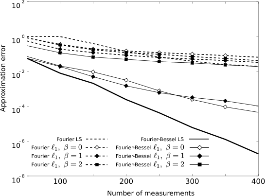
Figure 5: Best reconstruction error for method (i) Fourier least-squares, (ii) Fourier Weighted Basis Pursuit, (iii) Fourier-Bessel least-squares (proposed method) and (iv) Fourier-Bessel Weighted Basis Pursuit

6 Further issues

We showed above that a careful choice of the sampling distribution allows us to use a larger order of approximation. However, in practice, the optimal value of $m$ is unknown to us. We test here the cross-validation method to estimate this value. We also estimate the value of $K(m)$ for a square and different sampling densities, and show that a non-uniform density on the border may be necessary in a general setting.

6.1 Estimation of the model order with the cross-validation method

For a given number $m=2L+1$ of Fourier-Bessel functions, we estimate a reconstruction using 95% of the samples, and evaluate empirically the mean-square error using the remaining ones. We repeat the estimation 10 times using different choices of estimation and reconstruction points within the same sample, and select the number $m$ that minimizes the mean square error. The function is then reconstructed using all samples. On Figure 6, we compare the results obtained by this method with those based on the optimal value of $m$, as the number of measurement $n$ varies. Here we use the sampling distribution according to the measure $\nu_{\alpha}$, with $\alpha=0.9$. We observe that the performances are comparable up to a slight loss by a multiplicative constant.

Figure 6: Best reconstruction error for the proposed method, using GCV and optimal value of $m$.

6.2 More general shapes

While the results obtained here inform us on the importance of sampling on the border of the considered domain, a numerical test on another simple shape shows that the density on the border is critical. The theoretical analysis for the disk and the ball was based on the fact that the Fourier-Bessel functions were already an orthogonal basis of the space $V_{m}^{b}$. We focus here on the square $[-1,1]^{2}$. As neither the Fourier-Bessel functions, nor the plane waves, form an orthogonal basis, we construct one by orthogonalizing the Fourier-Bessel functions.

We numerically compute $K(m)$ for four different distributions:

• $\nu_{0}=ds$, the uniform distribution on the square,

• $\nu^{\prime}=4ds/\left(\pi^{2}\sqrt{1-x^{2}}\sqrt{1-y^{2}}\right)$, a distribution denser near the edges and corners of the square,

• $\nu_{\alpha}=(1-\alpha)ds+\alpha d\sigma$, where $\sigma$ is the uniform distribution on the boundary of the square,

• $\nu^{\prime}_{\alpha}=(1-\alpha)ds+\alpha d\sigma^{\prime}$, where $d\sigma^{\prime}$ is the measure on the boundary with weight $1/4\pi\sqrt{1-s^{2}}$ where $s=\min(x,y)$ (i.e. denser near the corners of the square).

Figure 7 shows examples of such distributions for $\alpha=1/2$.

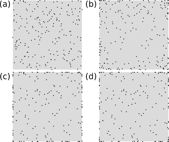
Figure 7: Examples of sampling distributions on the square: (a) $\nu$, (b) $\nu^{\prime}$, (c) $\nu_{1/2}$, (d) $\nu^{\prime}_{1/2}$.

The estimated values of $K(m)$ for $\nu_{0}$, $\nu^{\prime}$, $\nu_{1/2}$ and $\nu^{\prime}_{1/2}$ are given on figure 8. Here, having a denser sampling near or on the border of the square improves the stability of the reconstruction compared to the uniform case, but still needs a high number of samples.

Using the non-uniform sampling on the border, with more samples in the sections of the boundary furthest from the origin, makes the behavior of $K(m)$ comparable to $m$, which is the best case possible.

Figure 8: Numerical evaluation of $K$ for four different samples distribution on the square.

7 Conclusion

In this paper, we compare different ways of sampling solutions to the Helmholtz equation, using a finite number of point measurements. Our main results reveal that good reconstructions can be obtained using Fourier-Bessel or plane waves approximations, and that these reconstructions benefit from a denser sampling on the boundary.

These results were obtained in the particular case of a two-dimensional disc or a three-dimensional ball. For a more general star-shaped domain in ${\mathbf{R}}^{2}$, the Fourier-Bessel approximation remains valid, but the quantity $K(m)$ does not have an explicit expression, yet it can be evaluated numerically after orthogonalization of the Fourier-Bessel or plane waves family. Our first numerical investigation, on the square, indicates that denser, but non-uniform, sampling of the functions on the boundary is also beneficial in this more general setting.

Finally, sampling of other physical quantities can benefit from similar sampling strategies, e.g. vibrations of plates [3, 2], electromagnetic fields [5], or vibrations in 3D linear elasticity [8]. Indeed, they can be approximated using schemes similar to the ones used here.

ACKNOWLEDGEMENT

This research is supported by the FWF START-project FLAME (Y 551-N13) and the ANR project ECHANGE (ANR-08-EMER-006). LD is partly supported by Institut Universitaire de France and by LABEX WIFI (Laboratory of Excellence within the French Program ”Investments for the Future”) under references ANR-10-LABX-24 and ANR-10-IDEX-0001-02 PSL.

References

- [1] M. Abramowitz and I.A. Stegun. Handbook of Mathematical Functions with Formulas, Graphs, and Mathematical Tables. Dover, New York, 1964.
- [2] G. Chardon and L. Daudet. Low-complexity computation of plate eigenmodes with vekua approximations and the method of particular solutions. Computational Mechanics, 52:983–992, 2013.
- [3] G. Chardon, A. Leblanc, and L. Daudet. Plate impulse response spatial interpolation with sub-Nyquist sampling. Journal of Sound and Vibration, 330(23):5678 – 5689, 2011.
- [4] Albert Cohen, Mark A. Davenport, and Dany Leviatan. On the stability and accuracy of least squares approximations. Foundations of Computational Mathematics, pages 1–16, 2013.
- [5] R. Hiptmair, A. Moiola, and I. Perugia. Error analysis of Trefftz-discontinuous Galerkin methods for the time-harmonic Maxwell equations. Math. Comp., 82:247–268, 2013.
- [6] A. Moiola, R. Hiptmair, and I. Perugia. Plane wave approximation of homogeneous Helmholtz solutions. Zeitschrift für Angewandte Mathematik und Physik (ZAMP), 62:809–837, 2011. 10.1007/s00033-011-0147-y.
- [7] A. Moiola, R. Hiptmair, and I. Perugia. Vekua theory for the Helmholtz operator. Zeitschrift für Angewandte Mathematik und Physik (ZAMP), 62:779–807, 2011. 10.1007/s00033-011-0142-3.
- [8] Andrea Moiola. Plane wave approximation in linear elasticity. Applicable Analysis, 92(6):1299–1307, 2013.
- [9] Y. C. Pati, R. Rezaiifar, and P. S. Krishnaprasad. Orthogonal matching pursuit: Recursive function approximation with applications to wavelet decomposition. In Proceedings of the 27 th Annual Asilomar Conference on Signals, Systems, and Computers, pages 40–44, 1993.
- [10] E. Perrey-Debain. Plane wave decomposition in the unit disc: Convergence estimates and computational aspects. Journal of Computational and Applied Mathematics, 193(1):140 – 156, 2006.
- [11] H. Rauhut and R. Ward. Interpolation via weighted minimization. arXiv:1308.0759.
- [12] E. van den Berg and M. P. Friedlander. SPGL1: A solver for large-scale sparse reconstruction, June 2007. http://www.cs.ubc.ca/labs/scl/spgl1.
- [13] E. van den Berg and M. P. Friedlander. Probing the Pareto frontier for basis pursuit solutions. SIAM Journ. Sc. Comp., 31(2), 2008.
- [14] Illia N. Vekua. New methods for solving elliptic equations. North-Holland, 1967.