Quantum Hertz entropy increase in a quenched spin chain

Abstract

The classical Hertz entropy is the logarithm of the volume of phase space bounded by the constant energy surface; its quantum counterpart, the quantum Hertz entropy, is $\hat{S}=k_{B}\ln\hat{N}$, where the quantum operator $\hat{N}$ specifies the number of states with energy below a given energy eigenstate. It has been recently proved that, when an isolated quantum mechanical system is driven out of equilibrium by an external driving, the change in the expectation of its quantum Hertz entropy cannot be negative, and is null for adiabatic driving. This is in full agreement with the Clausius principle. Here we test the behavior of the expectation of the quantum Hertz entropy in the case when two identical $XY$ spin chains initially at different temperatures are quenched into a single $XY$ chain. We observed no quantum Hertz entropy decrease. This finding further supports the statement that the quantum Hertz entropy is a proper entropy for isolated quantum systems. We further quantify how far the quenched chain is from thermal equilibrium and the temperature of the closest equilibrium.

1 Introduction

The recent tremendous development in the field of nonequilibrium quantum fluctuations Campisi11RMP83 ; Esposito09RMP81 , has unveiled with an unprecedented clarity that many phenomena traditionally associated exclusively with macroscopic thermodynamic behaviour may manifest themselves even at the microscopic quantum level. Notably, the Second Law of thermodynamics, in the work-free energy formulation Fermi56Book ,

$$\langle w\rangle\geq\Delta F\,,$$ (1)

holds down to the quantum level Allahverdyan02PHYSA305 . In Eq. (1), $w$ is the work done on a quantum system that is initially in equilibrium with a thermal bath, when the system is perturbed by an external time dependent protocol that changes its Hamiltonian in time. The brackets indicate average over many realizations, and $\Delta F$ is the difference between the free energy of a hypothetical equilibrium state (not necessarily reached by the system) corresponding to the final Hamiltonian, and the actual initial free energy of the system. Eq. (1) follows straightforwardly from the quantum version of the Jarzynski identity Jarzynski97PRL78 ; Tasaki00arXiv ; Kurchan00arXiv ; Talkner07JPA40 .

For a cyclical driving, $H(\tau)=H(0)$, $\Delta F=0$, Eq. (1) says, in accordance with Kelvin postulate, that no energy can be extracted by the cyclic variation of a parameter from a system in contact with a single bath Allahverdyan02PHYSA305 :

$$\langle w\rangle\geq 0\quad\text{Kelvin (cyclic, with bath)}$$ (2)

Given the recent theoretical and experimental advances concerning the nonequilibrium dynamics of isolated quantum systems Polkovnikov11RMP83 , an interesting question is whether a microscopic quantum formulation of the second law in accordance with Clausius formulation, is possible as well. According to Clausius’ formulation the change of entropy of a thermally insulated driven system, which begins and ends in equilibrium, is non-negative:

$$\Delta S\geq 0\quad\text{Clausius (no bath)}$$ (3)

Answering this question is not a simple task because it amounts to singling out a quantum mechanical quantity that behaves as prescribed by the Clausius principle and goes over to the usual thermodynamic entropy in the classical/thermodynamic limit. Of course von Neumann “entropy”, $-\text{Tr}\rho\log\rho$, proves inadequate in this respect because it is invariant under the quantum unitary time evolution.

One proposal in the direction of answering the above question was put forward by Polkovnikov Polkovnikov11AP326 ; Santos11PRL107 , with the introduction of the so-called diagonal entropy. Another proposal, put forward by Hal Tasaki and by one of us Tasaki00arXivb ; Campisi08SHPMP39 ; Campisi08PRE78b , uses instead the Hertz entropy Hertz10AP338a ; Campisi05SHPMP36 ; Campisi10AJP78 see Eq. (4), or in quantum mechanics, its quantum counterpart, that is the logarithm of the “quantum number operator” $\hat{N}$ Tasaki00arXivb ; Campisi08SHPMP39 ; Campisi08PRE78b , see Eq. (5) below. In Tasaki00arXivb ; Campisi08SHPMP39 ; Campisi08PRE78b it was shown that the expectation of the quantum Hertz entropy behaves in accordance to the Clausius principle. Here we scrutinize whether it complies also with another property of thermodynamic entropy, namely whether it increases in a scenario when two quantum systems initially at different temperatures are allowed to exchange energy via the sudden switch-on of an interaction. This is a scenario that has recently attracted considerable attention Ponomarev11PRL106 ; Ponomarev12EPL98 , and that, given the recent advances, e.g., in ultra-cold-atom physics Bloch08RMP80 , is amenable to experimental investigations.

In our study the two interacting bodies are two isotropic $XY$ spin chains of length $N/2$, which are initially at different temperatures, and are suddenly quenched into a single isotropic $XY$ spin chain of length $N$. While the quench dynamics in spin-chains has been thoroughly studied, only few studies addressed their thermodynamics Campisi10CP375 ; Dorner12PRL109 .

In Secs. 2 and 3 we review the quantum Hertz entropy and present our model, respectively. In Secs. 4 and 5 we calculate the initial and final expectation of the quantum Hertz entropy. Results concerning the entropy change and the deviation of the final state from thermal equilibrium are presented in Sec. 6 and Sec. 7, respectively. Conclusions are drawn in Sec. 8.

2 Quantum Hertz entropy

The microcanonical entropy of a classical system is the so-called Hertz entropy Hertz10AP338a ; Campisi05SHPMP36 ; Campisi10AJP78 ; Hilbert06PRE74 presented also by Gibbs in his classic book GibbsBook , namely

$$S=k_{B}\ln[\Phi/h^{f}]\,,$$ (4)

where $k_{B}$ is Boltzmann constant, $\Phi$ is the phase space volume enclosed by the hyper-surface of constant energy in the system phase space of dimension $2f$ and $h$ is Planck’s constant. According to semiclassical reasoning LandauBook5 , in the quantum limit, the quantity $\Phi/h^{f}$ gets the discrete values $n=1,2,\dots$ . The associated quantum operator is the quantum number operator $\hat{N}$, whose eigenvectors are the energy eigenvectors, with the integers the corresponding eigenvalues. For a driven system, the operator $\hat{N}$ is time dependent, and its spectral decomposition reads (for non degenerate Hamiltonians) $\hat{N}(t)=\sum n\Pi_{n}(t)$, with $\Pi_{n}(t)$ the instantaneous eigenprojectors on the eigenspace spanned by the instantaneous eigenvalue $E_{n}(t)$ of the Hamiltonian $H(t)$. Here it is assumed that the energy eigenvalues are non-degenerate and ordered in increasing fashion: $E_{1}(t)<E_{2}(t)<\dots$ . Accordingly, the quantum mechanical operator associated to the Hertz entropy is

$$\hat{S}(t) =k_{B}\ln\hat{N}(t)\,.$$ (5)

Under the assumption that (i) the density matrix $\rho(0)$ describing the initial state of the system is diagonal in the energy eigenbasis $\rho(0)=\sum p_{n}\Pi_{n}(0)$, and (ii) the population $p_{n}$ decreases with increasing energy (i.e., $p_{n}\leq p_{m}$, if $E_{n}(0)>E_{m}(0)$); it has been shown that Tasaki00arXivb ; Campisi08SHPMP39 ; Campisi08PRE78b :

$$S(t)\geq S(0)\,,$$ (6)

where

$$S(t) =\text{Tr}\hat{S}(t)\rho(t)\,.$$ (7)

For adiabatic transformations the equal sign holds in Eq. (6). The quantity $S(t)$ hence behaves in accordance to the Clausius principle and goes over to the usual thermodynamic entropy in case of large classical systems at equilibrium. These facts make it a sound quantum mechanical counterpart for the thermodynamic entropy of a thermally insulated system. In the following we shall refer to $S$ and $\hat{S}$ as to the quantum entropy, and the quantum entropy operator, respectively. Note however that unless the system is in equilibrium at time $t$, the quantum entropy $S(t)$ should not be considered as the thermodynamic entropy of the system. The latter is an exclusively equilibrium property.

2.1 Remarks

We remark that unlike the Boltzmann entropy $S_{B}=k_{B}$ $\log[\Omega/h^{f}]$, [$\Omega=\partial_{E}\Phi$ being the density of states], the Hertz entropy is not postulated, but rather rationally derived from the fundamental requirement that its differential $dS$ exactly equals the quantity $\delta Q/T$ as calculated in the microcanonical ensemble, the so-called generalized Helmholtz theorem Campisi05SHPMP36 ; Campisi10AJP78 . As such, at equilibrium, the Hertz entropy has to be identified with the thermodynamic entropy. It is commonly assumed that $S$ and $S_{B}$ are equivalent Huang87Book , which is true in most cases but has important exceptions, e.g., in small systems or systems with a finite spectrum. In this latter case they can give drastically different results, notably $S$, a monotonically increasing function of $E$, gives only positive temperatures in accordance to thermodynamic fundamentals Callen60Book , whereas $S_{B}$ predicts also negative ones. This is a topic of current interest as testified by recent experiments Braun13SCIENCE339 .

For a Gibbs ensemble of systems at canonical temperature $T_{c}=1/k_{B}\beta$, one finds the following expression for the work dissipated, $W_{\text{diss}}=\langle w\rangle-\Delta F$, due to an external driving Schloegl66ZP191 ; Bochkov81aPHYSA106 ; Kawai07PRL98 ; Deffner10PRL105 :

$$W_{\text{diss}} =k_{B}T_{c}D[\rho(t)|\rho^{\text{eq}}(t)]$$ (8)

where $D[\rho(t)|\rho^{\text{eq}}(t)]=\text{Tr}\rho(t)\log\rho(t)-\text{Tr}\rho(t)\log\rho^{\text{eq}}(t)$ is the Kullbeck-Leibler divergence between $\rho(t)$, the density matrix of the system at time $t$, and $\rho^{\text{eq}}(t)=e^{-\beta H(t)}/\text{Tr}e^{-\beta H(t)}$ the corresponding equilibrium density matrix. The quantity $W_{\text{diss}}/T_{c}=k_{B}D[\rho(t)|\rho^{\text{eq}}(t)]$ is often referred to as the entropy production Crooks99PRE60 . This off-equilibrium quantity should not be confused with the change in thermodynamic entropy $\int\delta Q/T$, which involves quasi-static heat exchanges, instead. However there exist a strict connection between $W_{\text{diss}}$ and the change in thermodynamic entropy $\Delta S$.

Noticing that the Kullbeck-Leibler divergence is a non-negative quantity, it is apparent from Eq. (8) that $W_{\text{diss}}\geq 0$ for $T_{c}>0$, $W_{\text{diss}}\leq 0$ for $T_{c}<0$. This can be easily obtained also from the Jarzynski identity Campisi11RMP83 . It says that when one perturbs a Gibbs ensemble of thermally isolated systems characterized by a positive canonical $T_{c}$, one gets out less energy than one puts in, on average. This is the second law in the usual Kelvin formulation. Vice-versa one gets out more energy than one puts in, if the ensemble was characterized by a negative $T_{c}$. This is well described by Ramsey’s account of the early experiments on negative spin temperatures. He writes (Ramsey56PR103, , see p. 27) “when a negative temperature spin system was subjected to resonance radiation more radiant energy was given off by the spin system than was absorbed.” In sum, it is an experimental fact that when perturbing canonical ensembles characterized by negative $T_{c}$, the second law is inverted. Accordingly the entropy should decrease, and this is in fact the behavior of the Hertz entropy Campisi08SHPMP39 : $\Delta S\geq 0$ for $T_{c}>0$, $\Delta S\leq 0$ for $T_{c}<0$, which shows the equivalence of Kelvin and Clausius formulations down to microscopic quantum level, and also to negative $T_{c}$’s.

One difference between the quantum Hertz entropy and the diagonal entropy Polkovnikov11AP326 is that the latter would always increase, regardless of the sign of $T_{c}$ of the initial canonical ensemble. Presumably the diagonal entropy does not differ much from the Hertz entropy in ordinary large systems with unbound spectrum. This question however deserves a detailed investigation that goes beyond the scope of the present contribution.

3 The Model

Our model consists of two identical isotropic XY spin chains, which are quenched at time $t=0$ to a single XY chain of twice the length, see Fig. 1.

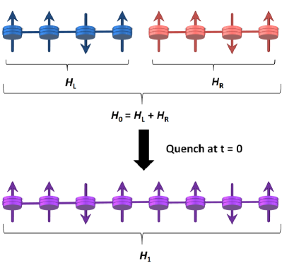
Figure 1: Schematics of our model

At times $t<0$, the system Hamiltonian is:

$$H_{0}=H_{L}+H_{R}\,,$$ (9)

with:

$$H_{L} =-\frac{h}{2}\sum_{j=1}^{N/2}{\sigma_{j}^{z}}+\frac{J}{2}\sum_{j=1}^{N/2-1}{[\sigma_{j}^{x}\sigma_{j+1}^{x}+\sigma_{j}^{y}\sigma_{j+1}^{y}]}\,,$$ (10)

$$H_{R} =-\frac{h}{2}\sum_{j=N/2+1}^{N}{\sigma_{j}^{z}}+\frac{J}{2}\sum_{j=N/2+1}^{N-1}{[\sigma_{j}^{x}\sigma_{j+1}^{x}+\sigma_{j}^{y}\sigma_{j+1}^{y}]}\,.$$ (11)

Here $\sigma_{j}^{\alpha}$, $j=1\dots N$, $\alpha=x,y,z$, denotes the Pauli matrices of the $j$-th spin. At $t<0$ the left (right) chain is in the Gibbs state of temperature $T_{L(R)}$, hence the total system density matrix is given by their product:

$$\rho_{0}=\frac{e^{-\beta_{L}H_{L}}}{Z(\beta_{L})}\otimes\frac{e^{-\beta_{R}H_{R}}}{Z(\beta_{R})}\,,$$ (12)

where $Z(\beta)=\text{Tr}e^{-\beta H_{L}}=\text{Tr}e^{-\beta H_{R}}$ is the partition function, and $\beta_{L(R)}=(k_{B}T_{L(R)})^{-1}$, with $k_{B}$ Boltzmann constant. At time $t=0$ an interaction between spin $N/2$ and spin $N/2+1$ is turned on, such that the Hamiltonian is, for $t>0$:

$$H_{1} =-\frac{h}{2}\sum_{j=1}^{N}{\sigma_{j}^{z}}+\frac{J}{2}\sum_{j=1}^{N-1}{[\sigma_{j}^{x}\sigma_{j+1}^{x}+\sigma_{j}^{y}\sigma_{j+1}^{y}]}\,.$$ (13)

The Hamiltonians $H_{L},H_{R},H_{1}$ all represent isotropic XY chains of different lengths. Following the standard procedures they can be put in diagonal form by means of Jordan-Wigner transformation followed by a sine transform Lieb61AP16 ; Mikeska77ZPB26 . Specifically

$$H_{1}=\sum_{j=1}^{N}\varepsilon_{k}b_{k}^{\dagger}b_{k}+\frac{Nh}{2}\,,$$ (14)

where

$$\varepsilon_{k} =-h-2J\cos\left(\frac{k\pi}{N+1}\right)\,,$$ (15)

$$b_{k} =\sqrt{\frac{2}{N+1}}\sum_{i=1}^{N}\sin\left(\frac{ki\pi}{N+1}\right)a_{i}\,,$$ (16)

$$a_{j} =\prod_{k=1}^{j-1}\sigma^{z}_{k}\sigma_{j}^{-}\,,$$ (17)

$$\sigma_{j}^{\pm} =\frac{1}{2}(\sigma^{x}_{j}\pm i\sigma^{y}_{j})\,;$$ (18)

We shall denote the eigenvectors and eigenvalues of $H_{1}$ as $|\bm{n}\rangle=|n_{1},n_{2},\dots n_{N}\rangle$ and $E_{\bm{n}}$, respectively, where $n_{i}=0,1$:

$$H_{1}|\bm{n}\rangle=E_{\bm{n}}|\bm{n}\rangle,\qquad E_{\bm{n}}=\sum_{k=1}^{N}\varepsilon_{k}n_{k}+\frac{Nh}{2}\,.$$ (19)

The states $|\bm{n}\rangle$ are the Fock states associated to the fermonic operators $b_{k}$. For future reference we recall their properties

$$b_{k}^{\dagger}b_{k}|...\,n_{k}\,...\rangle =n_{k}|...\,n_{k}\,...\rangle$$ (20)

$$b_{k}|...\,n_{k}\,...\rangle =n_{k}(-1)^{\sum_{i=1}^{k-1}n_{i}}|...\,n_{k}-1\,...\rangle$$ (21)

$$b_{k}^{\dagger}|...\,n_{k}\,...\rangle =(1-n_{k})(-1)^{\sum_{i=1}^{k-1}n_{i}}|...\,n_{k}+1\,...\rangle$$ (22)

Similarly, for the $L$-chain:

$$H_{L} =\sum_{k=1}^{N/2}\varepsilon^{\prime}_{k}b_{k}^{\prime\dagger}b^{\prime}_{k}+\frac{Nh}{4}\,,$$ (23)

$$\varepsilon_{k}^{\prime} =-h-2J\cos\left(\frac{k\pi}{N/2+1}\right)\,,$$ (24)

$$b^{\prime}_{k} =\sqrt{\frac{2}{N/2+1}}\sum_{i=1}^{N/2}\sin\left(\frac{ki\pi}{N/2+1}\right)a_{i}\,.$$ (25)

Note that the same Jordan-Wigner operators $a_{i}$ are used for the $L$-chain and the total chain. In defining $b_{k}$ all $N$ operators are used, while only the first $N/2$ are employed to define the primed operators $b^{\prime}_{k}$. We shall denote the eigenvectors and eigenvalues of $H_{L}$ as $|\bm{l}\rangle=|l_{1},l_{2},\dots l_{N/2}\rangle$ and $E_{\bm{l}}$, respectively:

$$H_{L}|\bm{l}\rangle=E_{\bm{l}}|\bm{l}\rangle,\qquad E_{\bm{l}}=\sum_{k=1}^{N/2}\varepsilon^{\prime}_{k}l_{k}+\frac{Nh}{4}\,.$$ (26)

Likewise for the $R$-chain,

$$H_{R} =\sum_{k=1}^{N/2}\varepsilon^{\prime}_{k}b_{k}^{\prime\prime\dagger}b^{\prime\prime}_{k}+\frac{Nh}{4}\,,$$ (27)

$$b^{\prime\prime}_{k} =\sqrt{\frac{2}{N/2+1}}\sum_{i=1}^{N/2}\sin\left(\frac{ki\pi}{N/2+1}\right)a^{\prime\prime}_{i}$$ (28)

$$a^{\prime\prime}_{j} =\prod_{k=1}^{j-1}\sigma^{z}_{N/2+k}\sigma_{N/2+j}^{-}$$ (29)

Note two prominent facts: i) the single mode eigenenergies $\varepsilon^{\prime}_{k}$ are the same for the $L$-chain and the $R$-chain, because the two chains are identical. (ii) The Jordan Wigner operators $a^{\prime\prime}_{j}$ of the $R$-chain differ from the Jordan Wigner operators $a_{j}$ of the $L$-chain and total chain, because the latter begin with spin $1$, while the $R$-chain begins with spin $N/2+1$. We shall denote the eigenvectors and eigenvalues of $H_{R}$ as $|\bm{r}\rangle=|r_{1},r_{2},\dots r_{N/2}\rangle$ and $E_{\bm{r}}$, respectively:

$$H_{R}|\bm{r}\rangle=E_{\bm{r}}|\bm{r}\rangle,\qquad E_{\bm{r}}=\sum_{k=1}^{N/2}\varepsilon^{\prime}_{k}r_{k}+\frac{Nh}{4}\,.$$ (30)

4 Initial quantum Entropy

At times $t<0$ the entropy of the two non-interacting chains is given by the sum of their individual entropies. We proceed by calculating the quantum entropy $S^{\beta}$ of the left chain at inverse thermal energy $\beta$. Since the two chains are identical this also gives the quantum entropy of right chain at the same inverse thermal energy $\beta$.

According to Eq. (7)

$$S^{\beta} =\frac{k_{B}}{Z(\beta)}\text{Tr}\,e^{-\beta H_{L}}\,\ln\hat{L}$$

$$=\frac{k_{B}}{Z(\beta)}\sum_{\bm{l}}\,e^{-\beta E_{\bm{l}}}\,\langle\bm{l}|\ln\hat{L}|\bm{l}\rangle$$

$$=\frac{k_{B}}{Z(\beta)}\sum_{\bm{l}}\,e^{-\beta E_{\bm{l}}}\,\ln\lambda_{\bm{l}}\,.$$ (31)

Here $\hat{L}$ is the principal quantum number operator associated to the $L$-chain. Its eigenvectors are the Fock states $|\bm{l}\rangle$, and its eigenvalues are $\lambda_{\bm{l}}$. The eigenvalues $\lambda_{\bm{l}}$ are calculated in the following way. The energy eigenvalues $E_{\bm{l}}$ are ordered accordingly to their increasing values, so as to obtain a sequence

$$E_{\bm{l}_{1}}<E_{\bm{l}_{2}}<\dots<E_{\bm{l}_{2^{N/2}}}\,,$$ (32)

where $|\bm{l}_{1}\rangle$ is the ground state, $|\bm{l}_{2}\rangle$ is the first excited state, $\dots$ $|\bm{l}_{2^{N/2}}\rangle$ is the state of highest energy. Then $\lambda_{\bm{l}_{1}}=1,\lambda_{\bm{l}_{2}}=2$, etc.

The total initial quantum entropy $S_{0}$, is given by:

$$S_{0}=S^{\beta_{L}}+S^{\beta_{R}}.$$ (33)

5 Final quantum entropy

Due to the assumption of sudden quench, at time $t=0^{+}$ the density matrix retains the initial form in Eq. (12). The final quantum entropy $S_{1}$ is therefore given by

$$S_{1} =k_{B}\frac{\text{Tr}\,e^{-\beta_{L}H_{L}}e^{-\beta_{R}H_{R}}\ln\hat{N}}{Z(\beta_{L})Z(\beta_{R})}$$

$$=k_{B}\frac{\sum_{\bm{n}}\langle\bm{n}|e^{-\beta_{L}H_{L}}e^{-\beta_{R}H_{R}}|\bm{n}\rangle\ln\nu_{\bm{n}}}{Z(\beta_{L})Z(\beta_{R})}\,.$$ (34)

Here $\hat{N}$ is the quantum number operator associated to the total chain, and $\nu_{\bm{n}}$ are its integer eigenvalues, obtained as described above for the smaller $L$-chain, with the difference that now one has to order the $2^{N}$ eigenvalues $E_{\bm{n}}$.

We next consider the basis $|\bm{l}\bm{r}\rangle=|\bm{l}\rangle\otimes|\bm{r}\rangle$ formed by the direct product of the eigenbasis of $H_{L}$ and $H_{R}$: Using the resolution of the identity $\sum_{\bm{l},\bm{r}}|\bm{l}\bm{r}\rangle\langle\bm{l}\bm{r}|=\mathbb{1}$, the final quantum entropy reads:

$$S_{1} =k_{B}\frac{\sum_{\bm{n},\bm{l},\bm{r}}P(\bm{n}|\bm{l},\bm{r})e^{-\beta_{L}E_{\bm{l}}}e^{-\beta_{R}E_{\bm{r}}}\ln\nu_{\bm{n}}}{Z(\beta_{L})Z(\beta_{R})}\,,$$ (35)

where

$$P(\bm{n}|\bm{l},\bm{r})=\langle\bm{n}|\bm{l}\bm{r}\rangle\langle\bm{l}\bm{r}|\bm{n}\rangle\,.$$ (36)

In order to calculate $P(\bm{n}|\bm{l},\bm{r})$ we consider the basis $|\bm{s}\rangle=|s_{1},s_{2}\dots,s_{N}\rangle=|s_{1}\rangle\otimes|s_{2}\rangle\otimes\dots\otimes|s_{N}\rangle$ formed by the direct product of the eigenstates $|s_{j}\rangle$ of the $z$ component of each spin operator: $\sigma^{z}_{j}|s_{j}\rangle=s_{j}|s_{j}\rangle$ with $s_{j}=\pm$. Employing the resolution of the identity twice we obtain:

$$P(\bm{n}|\bm{l},\bm{r}) =\sum_{\bm{s},\bm{s}^{\prime}}\langle\bm{n}|\bm{s}\rangle\langle\bm{s}|\bm{l}\bm{r}\rangle\langle\bm{l}\bm{r}|\bm{s}^{\prime}\rangle\langle\bm{s}^{\prime}|\bm{n}\rangle$$

$$=\sum_{\bm{s},\bm{s}^{\prime}}\langle\bm{n}|\bm{s}\rangle\langle\bm{s}^{\prime}|\bm{n}\rangle\langle\bm{l}\bm{r}|\bm{s}^{\prime}\rangle\langle\bm{s}|\bm{l}\bm{r}\rangle\,.$$ (37)

The next crucial step in the calculation consists in expressing the operators $|\bm{s}\rangle\langle\bm{s}^{\prime}|$ in terms of spin rising and lowering operators. For a single spin, say spin $j$, we have $|+\rangle\langle+|=\sigma_{j}^{+}\sigma_{j}^{-}\,,|-\rangle\langle-|=\sigma_{j}^{-}\sigma_{j}^{+}\,,|+\rangle\langle-|=\sigma_{j}^{+}\,,|-\rangle\langle+|=\sigma_{j}^{-}$ which can be compactly written

$$|s\rangle\langle s^{\prime}|=\delta_{ss^{\prime}}\sigma_{j}^{s}\sigma_{j}^{-s}+(1-\delta_{ss^{\prime}})\sigma_{j}^{s}\,,$$ (38)

where $\delta_{ss^{\prime}}$ denotes the Kronecker symbol, and $\sigma_{j}^{\pm}$ are given in Eq. (18). Therefore:

$$|\bm{s}\rangle\langle\bm{s}^{\prime}|=\prod_{j}[\delta_{s_{j}s_{j}^{\prime}}\sigma_{j}^{s_{j}}\sigma_{j}^{-s_{j}}+(1-\delta_{s_{j}s_{j}^{\prime}})\sigma_{j}^{s_{j}}]\,.$$ (39)

In order to calculate $\langle\bm{n}|\bm{s}\rangle\langle\bm{s}^{\prime}|\bm{n}\rangle$ we express $|\bm{s}\rangle\langle\bm{s}^{\prime}|$ in terms of the fermionic operators $b_{k}$ of the total system. This can be accomplished by using the inverse sine transforms:

$$a_{j} =\sqrt{\frac{2}{N+1}}\sum_{k=1}^{N}\sin\left(\frac{kj\pi}{N+1}\right)b_{k}\,,$$ (40)

and the following identities:

$$\sigma_{j}^{s}\sigma_{j}^{-s} =a_{j}^{s}a_{j}^{-s}\,,$$ (41)

$$\sigma_{j}^{-s} =\prod_{k=1}^{j-1}(2a_{k}^{+}a_{k}^{-}-1)a_{j}^{-s}\,,$$ (42)

where we set the convenient notations $a_{j}^{+}\doteq a_{j}^{\dagger}$, $a_{j}^{-}\doteq a_{j}$. By plugging Eqs. (40, 41, 42) into Eq. (39), the operator $|\bm{s}\rangle\langle\bm{s}^{\prime}|$ is expressed in terms of the operators $b_{k}$ and $b_{k}^{\dagger}$. The wanted term $\langle\bm{n}|\bm{s}\rangle\langle\bm{s}^{\prime}|\bm{n}\rangle$ is calculated then by using the properties (20-22) and the orthonormality condition $\langle\bm{n}|\bm{n}^{\prime}\rangle=\delta_{n_{1},n_{1}^{\prime}}\delta_{n_{2},n_{2}^{\prime}}\dots\delta_{n_{N},n_{N}^{\prime}}$.

In order to calculate $\langle\bm{l}\bm{r}|\bm{s}^{\prime}\rangle\langle\bm{s}|\bm{l}\bm{r}\rangle$ we proceed by expressing $|\bm{s}\rangle$ as the direct product of two subchain states $|\bm{s}\rangle=|s_{1}\dots s_{N}\rangle=|s_{1}\dots s_{N/2}\rangle\otimes|s_{N/2+1}\dots s_{N}\rangle=|\bm{s}_{L}\rangle\otimes|\bm{s}_{R}\rangle$. Accordingly, the wanted term reduces to the product of two terms each pertaining to each subchain: $\langle\bm{l}\bm{r}|\bm{s}^{\prime}\rangle\langle\bm{s}|\bm{l}\bm{r}\rangle$ $=\langle\bm{l}|\bm{s}^{\prime}_{L}\rangle\langle\bm{s}_{L}|\bm{l}\rangle\cdot\langle\bm{r}|\bm{s}^{\prime}_{R}\rangle\langle\bm{s}_{R}|\bm{r}\rangle$. The calculation of $\langle\bm{l}|\bm{s}^{\prime}_{L}\rangle\langle\bm{s}_{L}|\bm{l}\rangle$ proceeds as the above calculation of $\langle\bm{n}|\bm{s}\rangle\langle\bm{s}^{\prime}|\bm{n}\rangle$, with the only difference that now all quantities pertain to the smaller $L$-chain. Since the $L$ and $R$ chains are identical this automatically gives also the $R$-chain term $\langle\bm{r}|\bm{s}^{\prime}_{R}\rangle\langle\bm{s}_{R}|\bm{r}\rangle$.

In the Appendix we provide further details on how these calculations were implemented.

6 Entropy change

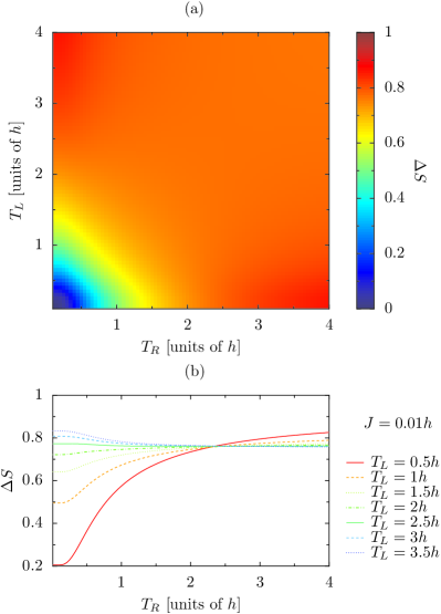
Figure 2: (a): Entropy change, Eq. (43), as a function of $T_{L},T_{R}$. (b): Entropy change, Eq. (43), as a function of $T_{R}$ for various fixed $T_{L}$’s. Here $h=1$, $J=0.01h$ and $N=8$.

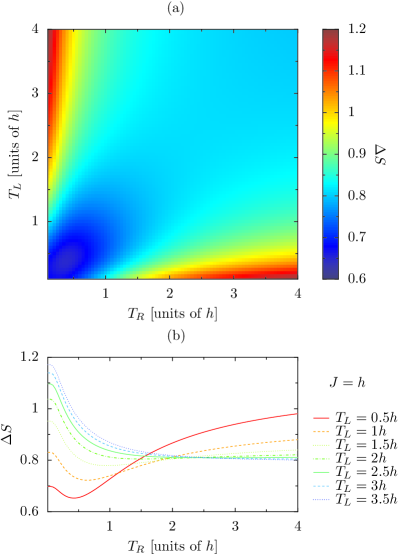
Figure 3: (a): Entropy change, Eq. (43), as a function of $T_{L},T_{R}$. (b): Entropy change, Eq. (43), as a function of $T_{R}$ for various fixed $T_{L}$’s. Here $h=1$, $J=h$ and $N=8$.

Using the method detailed above, we have calculated the change of quantum entropy

$$\Delta S=S_{1}-S_{0}$$ (43)

caused by the sudden quench, for different values of the parameters defining our problem. These are the initial temperatures of the left and right chains, $k_{B}T_{L,R}=\beta_{L,R}^{-1}$, the length $N$ of the total chain, and the interaction strength $J$. The field strength $h$ was used as the unit of energy, and we adopted the convention that temperatures are measured in units of energy. In these units we have $k_{B}$, Boltzmann’s constant, equal to $1$.

Figure 2, top panel, shows a surface plot of the entropy change in a chain of length $N=8$ at $J=0.01h$, as a function of $T_{L}$ and $T_{R}$. Figure 2, bottom panel, shows for the same values of $N=8,J=0.01h$, the behavior of $\Delta S$ as function of $T_{R}$ for various left chain temperatures $T_{L}=0.5h$ to $3.5h$. The quantum entropy change here is always positive and approaches a saturation value as $T_{R}$ becomes very large. We see qualitatively different behaviors of $\Delta S$ as a function of $T_{R}$, depending on $T_{L}$. As $T_{L}$ increases, $\Delta S$ changes from a monotonically increasing function of $T_{R}$ to a monotonically decreasing function of $T_{R}$. The transition occurs for $T_{L}$ of the order of the width of the spectrum of $H_{L}$ (which takes on the value $2.6h$ in this case).

In Fig. 3 we report the same quantities as in Fig. 2 with the only difference that now $J=h$. For this value $J=h$ the quantum entropy change, seen as a function of $T_{R}$ features minima for small values of $T_{L}$ and a monotonically decreasing behavior for large $T_{L}$. As with Fig. 2 the transition occurs for $T_{L}$ of the order of the width of the spectrum of $H_{L}$ (which is $2h$ in this case).

In both Fig. 2 and 3, we see a common feature. The values of $\Delta S$ corresponding to lower $T_{L}$ is smaller than the value of $\Delta S$ corresponding to larger $T_{L}$ at lower $T_{R}$, whereas it is vice-versa at larger values of $T_{R}$. We observed a similar behavior also at other values of $J$ (e.g., for $J=0.0001,0.1,2,5$) and $N=2,4,6$ for same value of all other parameters). In no case have we observed a negative change in quantum entropy.

For $T_{L}=T_{R}$, $\Delta S$ gives the entropy of mixing. In the high temperature limit $T_{L}=T_{R}\gg\Delta E$, where $\Delta E$ is the width of the spectrum, one gets $\Delta S=2^{-N}\ln(2^{N}!)-2^{-N/2+1}\ln({2^{N/2}!})$. For $N=8$, as in Figs. 2 and 3, this gives $\Delta S\simeq 0.72$. For large $N$, using Stirling approximation one gets $\Delta S\simeq 1$. The mixing entropy is non-zero because the spin chain is made of distinguishable particle (one can distinguish one spin from the other by its site label). It is however negligibly small as compared to the entropy itself, which is of order $N$, because it is a surface effect, and as such is of order 1.

7 Thermalization

After the quench, the system is in an out-of-equilibrium state. In order to quantify how far the system is from an equilibrium Gibbs state, one can employ one of the many metrics in the space of density matrices discussed in the literature, e.g., in reference Dajka11QIP10 . Among them the Hilbert-Schmidt distance:

$$D_{HS}[\rho,\sigma]=\sqrt{\text{Tr}(\rho-\sigma)^{2}}$$ (44)

appears best suited to the problem at hand. The reason is that, in our problem, the Hilbert-Schmidt distance between the after-quench density matrix $\rho_{t}$ and a Gibbs state

$$\rho_{\beta}=e^{-\beta H_{1}}/Z_{1}(\beta)\,,$$ (45)

where $Z_{1}(\beta)=\text{Tr}\,e^{-\beta H_{1}}$, does not depend on time $t$. Furthermore it can be calculated by knowing the initial density matrix $\rho_{0}$, Eq. (12), and the transition amplitudes $P(\bm{n},\bm{lr})$, Eq. (37). That is, it can be obtained from the only knowledge of the (time independent) diagonal elements

$$\langle\bm{n}|\rho_{t}|\bm{n}\rangle=\sum_{\bm{lr}}P(\bm{n}|\bm{l},\bm{r})\frac{e^{-\beta_{L}E_{\bm{l}}}e^{-\beta_{R}E_{\bm{r}}}}{Z(\beta_{L})Z(\beta_{R})}\,,$$ (46)

with no need to calculate the off-diagonal elements
$\langle\bm{n}|\rho_{t}|\bm{m}\rangle$, $\bm{n}\neq\bm{m}$. In fact:

$$D_{HS}^{2}[\rho_{t},\rho_{\beta}]=\text{Tr}\rho_{\beta}^{2}-2\text{Tr}\rho_{t}\rho_{\beta}+\text{Tr}\rho_{t}^{2}\,,$$ (47)

and

$$\text{Tr}\rho_{\beta}^{2} =\sum_{\bm{n}}\frac{e^{-2\beta E_{\bm{n}}}}{Z_{1}^{2}(\beta)}\,,$$ (48)

$$\text{Tr}\rho_{t}\rho_{\beta} =\sum_{\bm{n}}\frac{e^{-\beta E_{\bm{n}}}}{Z_{1}(\beta)}\langle\bm{n}|\rho_{t}|\bm{n}\rangle\,,$$ (49)

$$\text{Tr}\rho_{t}^{2} =\text{Tr}\rho_{0}^{2}=\sum_{\bm{rl}}\frac{e^{-2\beta_{L}E_{\bm{l}}}}{Z^{2}(\beta_{L})}\frac{e^{-2\beta_{R}E_{\bm{r}}}}{Z^{2}(\beta_{R})}\,.$$ (50)

Using Eqs. (44-50) we calculated the minimal distance

$$D_{HS}^{\text{min}}=\min_{\beta}D_{HS}[\rho_{t},\rho_{\beta}]\,,$$ (51)

between the final state $\rho_{t}$ and the set of thermal Gibbs states. This gives both an estimate of how far the system is from equilibrium, and what the temperature $k_{B}\bar{T}={\bar{\beta}}^{-1}$ is of the closest equilibrium, where $\bar{\beta}$ is the value of $\beta$ for which the minimum distance $D_{HS}^{\text{min}}$ is attained.

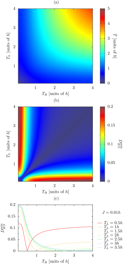
Figure 4: (a): Temperature $\bar{T}$ of closest equilibrium, as a function of $T_{L},T_{R}$. (b): Minimal distance $D_{HS}^{\text{min}}$, Eq. (51), as a function of $T_{R},T_{R}$. (c): Minimal distance $D_{HS}^{\text{min}}$, Eq. (51), as a function of $T_{R}$ for various fixed $T_{L}$’s. Here $h=1$, $J=0.01h$ and $N=8$.

Figure 5: (a): Temperature $\bar{T}$ of closest equilibrium, as a function of $T_{L},T_{R}$. (b): Minimal distance $D_{HS}^{\text{min}}$, Eq. (51), as a function of $T_{R},T_{R}$. (c): Minimal distance $D_{HS}^{\text{min}}$, Eq. (51), as a function of $T_{R}$ for various fixed $T_{L}$’s. Here $h=1$, $J=h$ and $N=8$.

Fig. 4 shows plots of $\bar{T}$ and $D_{HS}^{\text{min}}$ (panels (a) and (b), respectively), as a function of $T_{L},T_{R}$, at a low value of interaction strength $J=0.01h$ and chain length $N=8$. Panel (c) presents $D^{\text{min}}_{HS}$ as function of $T_{R}$ for various fixed $T_{L}$’s. Panel (b) indicates that better thermalization is achieved when $T_{L}$ and $T_{R}$ are closer. As can be seen from panel (a), when $T_{L}=T_{R}$ it is $\bar{T}\simeq T_{L}=T_{R}$. For fixed $T_{L}$ (panel (c)) we observe that as $T_{R}$ grows from zero, the minimal distance $D^{\text{min}}_{HS}$ first decreases, then reaches a minimum, and finally grows. The minimum is in correspondence to $T_{R}\sim T_{L}$ as expected, and it is sharper for low $T_{L}$’s.

Fig. 5 is like Fig. 4 with the only difference that it is for a larger interaction strength $J=h$. As compared with Fig. 4 we observe here a different structure of the plot of $D^{\text{min}}_{HS}$ as a function of $T_{L}$ and $T_{R}$, see panel (b). Within the range of $T_{L}$, $T_{R}$ considered in the plot, it appears that a smaller distance is achieved when either $T_{L}$, $T_{R}$ or both grow. This different structure is reflected in the curves presented in panel (c), presenting $D^{\text{min}}_{HS}$ as a function of $T_{R}$, for fixed $T_{L}$’s. The structure of the plot of $\bar{T}$ as a function of $T_{L},T_{R}$, panel (a), is qualitatively similar to the corresponding plot in Fig. 4. Note that for $T_{L}=T_{R}$, the temperature of the closest equilibrium is larger than $T_{L}$, of some amount of the order of $h$. This is because the quench injects an energy amount of the order $J=h$ in the system. Similarly, in Fig. 4, $\bar{T}$ was close to $T_{L}=T_{R}$ because the quench injects in that case an energy of the order $J=0.01h$.

8 Conclusions

We have investigated numerically the change in the quantum Hertz entropy of Eq. (5), caused by a quench of two spin-chains of different temperatures into a larger single chain. Although we cannot conclude that such changes are always positive, our numerics clearly suggests that this is the typical behavior, thus providing further support to the statement that the quantum Hertz entropy of Eq. (5) is a proper quantum entropy for thermally isolated systems.

We further quantified how far the system is from equilibrium after the quench, and estimated the corresponding temperature of the closest equilibrium. For those quenches ending very close to an equilibrium state, it becomes meaningful to assign the system the equilibrium temperature $\bar{T}$, and the thermodynamic entropy $S_{1}$.

The Hertz entropy $S$ can be employed to study phase transitions and critical points in spin chains in a way analogous to Ref. Dorner12PRL109 where the dissipated work $W_{\text{diss}}$ signaled the crossing of a critical point as the magnetic field was incrementally and globally changed, and the chain was initially at some temperature $T$. Because of the strict connection between Hertz entropy and dissipated work, the Hertz entropy in that same scenario should give similar results. The present thermalization scenario, with an initial nonequilibrium state and a local quench, is not convenient though, for the study of critical points.

Acknowledgements

This work was supported by the DAAD-WISE 2011 Scholarship (D.G.J), the German-Israeli Foundation via grant no. G 1035-36.14/2009 (D.G.J) and the German Excellence Initiative Nanosystem Initiative Munich (M.C). D.G.J expresses sincere thanks to IISER, Pune, India for providing this great opportunity. D.G.J. would like to thank Prof. P. Hänggi (University of Augsburg) for the kind hospitality in his group. D.G.J. is also thankful to his friend Shadab Alam for fruitful discussions related to numeric.

Appendix

As detailed in Sec. 5, the transition probabilities $P(\bm{n}|\bm{l},\bm{r})$, involve the calculation of the expectation of the operators $|\bm{s}\rangle\langle\bm{s}^{\prime}|$ over the Fock states $|\bm{n}\rangle$. Accordingly, we have detailed how these operators may be expressed in terms of the fermonic operators $b_{k}$, whose action on the Fock states is defined in Eqs. (20,21,22). In order to calculate those expectations we expressed the fermionic operators $b_{k}$ in matrix form. First we represented the Fock states $|\bm{n}\rangle$ as tensorial product of single-spin states:

$$|0\rangle=\left(\begin{array}[]{clrr}0\\ 1\end{array}\right)\,,\qquad|1\rangle=\left(\begin{array}[]{clrr}1\\ 0\end{array}\right)\,.$$ (56)

For example, the Fock state $|01\rangle$ of a chain of $N=2$ spins read

$$|01\rangle =\left(\begin{array}[]{clrr}0\\ 1\end{array}\right)\otimes\left(\begin{array}[]{clrr}1\\ 0\end{array}\right)=\left(\begin{array}[]{clrr}0\\ 0\\ 1\\ 0\end{array}\right)$$ (65)

and similarly for larger chains. In this representation, the searched fermionic operators are represented by the following matrix tensorial products:

$$b_{k} =(-1)^{k-1}\underbrace{\sigma^{z}\otimes\ldots\otimes\sigma^{z}}_{\mbox{$k-1$ terms}}\,\otimes\,{\sigma^{-}}\otimes\,\underbrace{\mathbb{1}\otimes\ldots\otimes\,\mathbb{1}}_{\mbox{$N-k$ terms}}$$ (66)

$$b_{k} =(-1)^{k-1}\underbrace{\sigma^{z}\otimes\ldots\otimes\sigma^{z}}_{\mbox{$k-1$ terms}}\,\otimes\,{\sigma^{+}}\otimes\,\underbrace{\mathbb{1}\otimes\ldots\otimes\,\mathbb{1}}_{\mbox{$N-k$ terms}}$$ (67)

where $\sigma^{\pm}=(\sigma^{x}\pm\sigma^{y})/2$ are rising and lowering operators, expressed in terms of the Pauli matrices $\sigma^{x,y,z}$, and $\mathbb{1}$ is the $2\times 2$ identity matrix.

The calculation of $P(\bm{n}|\bm{l},\bm{r})$ further requires the calculation of the expectations $\langle\bm{l}|\bm{s}_{L}\rangle\langle\bm{s}^{\prime}_{L}|\bm{l}\rangle$, $\langle\bm{r}|\bm{s}_{R}\rangle\langle\bm{s}^{\prime}_{R}|\bm{r}\rangle$. The calculation of these proceeds exactly in the same way detailed above, with the only difference that the chain length is now $N/2$ instead of $N$. With all these expectations one can calculate the probabilities $P(\bm{n}|\bm{l},\bm{r})$, and, in turn, via Eq. (35), the final quantum entropy.

The performance of the calculation can be greatly improved if one notices the following selection rules

$$2\sum_{k=1}^{N}{n_{k}}\neq\sum_{j=1}^{N}{s_{j}}+N\implies\langle\bm{n}|\bm{s}\rangle=0\,,$$ (69)

$$2\sum_{k=1}^{N/2}{l_{k}}\neq\sum_{j=1}^{N/2}{s_{j}}+N/2\implies\langle\bm{l}|\bm{s}_{L}\rangle=0\,,$$ (70)

$$2\sum_{k=1}^{N/2}{r_{k}}\neq\sum_{j=N/2+1}^{N}{s_{j}}+N/2\implies\langle\bm{r}|\bm{s}_{R}\rangle=0\,.$$ (71)

Together with Eq. (37) these rules imply that the quench at time $t=0$ conserves the number of excitations.

References

- (1) M. Campisi, P. Hänggi, P. Talkner, Rev. Mod. Phys. 83, 771 (2011); 83 1653(E) (2011).
- (2) M. Esposito, U. Harbola, S. Mukamel, Rev. Mod. Phys. 81, 1665 (2009)
- (3) E. Fermi, Thermodynamics (Dover, New York, 1956)
- (4) A.E. Allahverdyan, T.M. Nieuwenhuizen, Physica A 305, 542 (2002)
- (5) C. Jarzynski, Phys. Rev. Lett. 78, 2690 (1997)
- (6) H. Tasaki, arXiv:cond-mat/0009244 (2000)
- (7) J. Kurchan, arXiv:cond-mat/0007360 (2000)
- (8) P. Talkner, P. Hänggi, J. Phys. A 40, F569 (2007)
- (9) A. Polkovnikov, K. Sengupta, A. Silva, M. Vengalattore, Rev. Mod. Phys. 83, 863 (2011)
- (10) A. Polkovnikov, Annals of Physics 326, 486 (2011)
- (11) L.F. Santos, A. Polkovnikov, M. Rigol, Phys. Rev. Lett. 107, 040601 (2011)
- (12) H. Tasaki, arXiv:cond-mat/0009206 (2000)
- (13) M. Campisi, Stud. Hist. Phil. Mod. Phys. 39, 181 (2008)
- (14) M. Campisi, Phys. Rev. E 78, 051123 (2008)
- (15) P. Hertz, Ann. Phys. (Leipzig) 338, 225 (1910)
- (16) M. Campisi, Stud. Hist. Phil. Mod. Phys. 36, 275 (2005)
- (17) M. Campisi, D.H. Kobe, Am. J. Phys. 78, 608 (2010)
- (18) A.V. Ponomarev, S. Denisov, P. Hänggi, Phys. Rev. Lett. 106, 010405 (2011)
- (19) A.V. Ponomarev, S. Denisov, P. Hänggi, J. Gemmer, EPL 98, 40011 (2012)
- (20) I. Bloch, J. Dalibard, W. Zwerger, Rev. Mod. Phys. 80, 885 (2008)
- (21) M. Campisi, D. Zueco, P. Talkner, Chem. Phys. 375, 187 (2010)
- (22) R. Dorner, J. Goold, C. Cormick, M. Paternostro, V. Vedral, Phys. Rev. Lett. 109, 160601 (2012)
- (23) S. Hilbert, J. Dunkel, Phys. Rev. E 74, 011120 (2006)
- (24) J. Gibbs, Elementary Principles in Statistical Mechanics (Yale U. P., New Haven, 1902)
- (25) L. Landau, E. Lifschitz, Statistical Physics, 2nd edn. (Pergamon, Oxford, 1969)
- (26) K. Huang, Statistical Mechanics, 2nd edn. (Wiley, New York, 1987)
- (27) H.B. Callen, Thermodynamics: an introduction to the physical theories of equilibrium thermostatics and irreversible thermodynamics (Wiley, New York, 1960)
- (28) S. Braun, J.P. Ronzheimer, M. Schreiber, S.S. Hodgman, T. Rom, I. Bloch, U. Schneider, Science 339, 52 (2013)
- (29) F. Schlögl, Z. Phys. 191, 81 (1966)
- (30) G.N. Bochkov, Y.E. Kuzovlev, Physica A 106, 443 (1981)
- (31) R. Kawai, J.M.R. Parrondo, C.V. den Broeck, Phys. Rev. Lett. 98, 080602 (2007)
- (32) S. Deffner, E. Lutz, Phys. Rev. Lett. 105, 170402 (2010)
- (33) G.E. Crooks, Phys. Rev. E 60, 2721 (1999)
- (34) R. Kubo, H. Ichimura, T. Usui, N. Hashitsume, Statistical Mechanics, 6th edn. (North Holland, Amsterdam, 1965)
- (35) N.F. Ramsey, Phys. Rev. 103, 20 (1956)
- (36) E. Lieb, T. Schultz, D. Mattis, Ann. Phys. 16, 407 (1961)
- (37) H.J. Mikeska, W. Pesch, Z. Phys. B 26, 351 (1977)
- (38) J. Dajka, J. Łuczka, P. Hänggi, Quantum Inf. Process. 10, 85 (2011)