Abstract

In this article, we have introduced a $\mathcal{PT}$ symmetric non-Hermitian Hamiltonian model which is given as $\hat{\mathcal{H}}=\omega(\hat{b}^{{\dagger}}\hat{b}+\frac{1}{2})+\alpha(\hat{b}^{2}-(\hat{b}^{{\dagger}})^{2})$ where $\omega$ and $\alpha$ are real constants, $\hat{b}$ and $\hat{b^{{\dagger}}}$ are first order differential operators. The Hermitian form of the Hamiltonian $\mathcal{\hat{H}}$ is obtained by suitable mappings and it is interrelated to the time independent one dimensional Dirac equation in the presence of position dependent mass. Then, Dirac equation is reduced to a Schrödinger-like equation and two new complex non-$\mathcal{PT}$ symmetric vector potentials are generated. We have obtained real spectrum for these new complex vector potentials using shape invariance method. We have searched the real energy values using numerical methods for the specific values of the parameters.

keyword: PT symmetry, pseudo-Hermiticity, Dirac equation.
PACS: 03.65.w, 03.65.Fd, 03.65.Ge.

1 Introduction

The nature of quantization arises due to the symmetry of the equations governing the physics. So, symmetry has long been known as a powerful and computational topic in quantum mechanics. Recently, there have been many studies of $\mathcal{PT}$ symmetric non-Hermitian systems with real energy since the original work of Bender and Boettcher [1] and the literature on such systems has expanded rapidly [2, 3, 4, 5, 6, 7]. One of the key points of the investigation was the $\mathcal{PT}$ symmetry generated by the product of the parity, $\mathcal{P}$, and time,$\mathcal{T}$ , linear and anti-linear inversion operators $\mathcal{P}x\mathcal{P}=-x$, $\mathcal{T}x\mathcal{T}=x$, $\mathcal{T}i\mathcal{T}=-i$. The operator $\mathcal{T}$ is anti-linear because it changes the sign of $i$. If $\mathcal{PT}$ symmetry of the Hamiltonian is unbroken; eigenfunction of the operator $\mathcal{PT}$ is simultaneously an eigenstate of Hamiltonian $H$, i.e. $[H,\mathcal{PT}]=0$. Later, it has been realized that the existence of real eigenvalues can be associated with a non-Hermitian Hamiltonian provided it is $\eta$-pseudo-Hermitian [8]: $\eta H=H^{{\dagger}}\eta$ where $\eta$ is a Hermitian linear automorphism which can be given as $\eta=(OO^{{\dagger}})^{-1}$, $O$ is a linear invertible operator. Here, the Hilbert space equipped with the inner product $<.,\eta.>$ is identified as the physical Hilbert space. And the observable $\Theta$ which is the element of physical Hilbert space is related to the Hermitian operator $\theta$ by means of a similarity transformation $\Theta=\rho^{-1}\theta\rho$ where $\rho=\eta^{2}$. At the same time Bagchi and Quesne have established that the twin concepts of pseudo-Hermiticity and weak-pseudo-Hermiticity [9]. Thus, the concept of pseudo-Hermiticity has attracted much interest on behalf of physicists [10, 11, 12, 13].

In [14], the Kepler problem solutions are investigated in Dirac theory for the particle whose mass is position dependent and the effective mass is given in the form of a multipole expansion, existence of the bound states are discussed in detail. Earlier, using a standard expansion of radial functions as a different approach, Dirac equation spectrum was obtained for the mixed potentials [15]. Results of [14] which are about large quantum numbers not leading to inverse mass and momentum independent energy is also consistent with those found in [16]. In [17], Dirac matrices $\hat{\alpha},\hat{\beta}$ have space factors as $f,f_{1}$ functions where $f$ responsible of the deformation of the Heisenberg algebra for the coordinates and momentum operators, $f_{1}$ is responsible of a dependence of the particle mass on its position. Exact solutions are found for the fermion in Coulomb field with the function $f$ which depends on $r$ linearly while the function $f_{1}$ depends on $r$ inversely. It is pointed out that the spectrum results of [17] can be useful for the nanoheterosystems. Similar arguments about the Dirac oscillator with deformed commutation relations leading to the existence of the minimal length of space can be found in [18].

Latterly, non-Hermitian potentials for the fermions have been studied in the literature [19, 20, 21, 22, 23] and fermion models interacting with $\mathcal{PT}$ symmetric potentials in presence of effective mass have been attracted interest [24, 25, 26, 27, 28, 29, 30]. In [31], the one-dimensional effective mass Dirac equation bound states are studied within the interactions of non-$\mathcal{PT}$-symmetric, and non-Hermitian, exponential type potentials. Moreover, $(1+1)$ Dirac equation with position-dependent mass (PDM) and complexified Lorentz scalar interactions, is discussed through the supersymmetric quantum mechanics [32]. More references about the complex potentials and Dirac theory can be found in [33].

Also, pseudo-Hermitian interaction in relativistic quantum mechanics is studied with the positive definite metric operator $\eta$ calculations for the state vectors [34]. Using the spin and pseudo-spin concept, spectrum of $PT$ symmetric Rosen-Morse potential is studied and analytical methods are used in [35]. Dirac equation with position dependent effective mass transformed into Schrödinger-like equation is studied in a general context and Lévai’s method is used [36]. Supersymmetric quantum mechanics (SUSY QM) provides elegant procedures to solve some classes of potentials with unbroken SUSY and shape invariance (SI) which is one of the standard way and it is known that the potential algebras of these systems have been investigated to find exact solutions [37, 38, 39, 40, 41, 42, 43, 44, 45, 46]. SUSY QM methods and relativistic extensions have been used by many authors [47, 48, 49, 50].

The purpose of the present paper is to explore new relativistic complex vector potentials of the non-Hermitian bosonic Hamiltonians which may be unsolvable and map them into a solvable but real effective potentials. In the literature, bosonic/fermionic Hamiltonians with two mode have physical importance such as Jaynes-Cummings model in solid-state physics [51], Bose-einstein condensate [52], squeezed states in a condensate of ultracold bosonic atoms confined by a double-well potential [53].

Using the methods of SUSY QM, we have obtained solutions of complex vector potentials and showed that in Dirac equation, decomposing the the vector potential into the real and imaginary parts leads to derive both exactly and conditionally exactly solvable potentials. The paper is organized as follows: In section $2$ a non-Hermitian Hamiltonian model is introduced by us and mapped into its Hermitian form. Shape invariance which is one of the effective tool in SUSY QM is given shortly in section $3$. Section $4$ includes the mapping of the Dirac equation into a Schrödinger-like equation and obtaining new complex and effective potentials with their exact solutions.

2 The Non-Hermitian Model and Hermitian Equivalents

Previous works by the authors have included many aspects of a non-Hermitian $su(2)$ Hamiltonian known as Swanson Hamiltonian [12, 54, 55, 56, 57, 58]. The Swanson Hamiltonian is given by $\hat{H}=\omega(\hat{a}^{{\dagger}}\hat{a}+1/2)+\alpha\hat{a}^{2}+\beta\hat{a^{{\dagger}}}^{2}$, where $\hat{a},\hat{a^{{\dagger}}}$ are annihilation and creation operators, $\omega,\alpha$ and $\beta$ are real constants. In this paper, let us consider a $\mathcal{PT}$ symmetric non-Hermitian model with two parameters given by

$$\hat{\mathcal{H}}=\omega(\hat{b}^{{\dagger}}\hat{b}+\frac{1}{2})+\alpha(\hat{b}^{2}-(\hat{b}^{{\dagger}})^{2})$$ (1)

where ${\dagger}$ is Hermitian adjoint, $\hat{b}$ is the annihilation operator given in a general form,

$$\hat{b}=A(x)\frac{d}{dx}+B(x)$$ (2)

and $A(x)$, $B(x)$ are real functions. $\mathcal{PT}$ operator has an effect as $x\rightarrow-x$, $p\rightarrow p$ and $i\rightarrow-i$ in the Hamiltonian, if the operators are taken as $\hat{b}=\frac{\omega}{2}\hat{x}+\frac{i}{2\omega}\hat{p}$, it can be seen that the Hamiltonian is $\mathcal{PT}$ symmetric. Now, in terms of differential operators, (1) becomes

$$\begin{split}\hat{\mathcal{H}}&=-\omega A(x)^{2}\frac{d^{2}}{dx^{2}}+(4\alpha A(x)B(x)-2\omega A(x)A(x)^{{}^{\prime}})\frac{d}{dx}\\ -&(\omega-2\alpha)A(x)B(x)^{{}^{\prime}}-(\omega-2\alpha)A(x)^{{}^{\prime}}B(x)+\omega B(x)^{2}-\alpha(A(x)A(x)^{{}^{\prime\prime}}+(A(x)^{{}^{\prime}})^{2})+\frac{\omega}{2}.\end{split}$$ (3)

We may write the eigenvalue equation for (1) as given below

$$\hat{\mathcal{H}}\psi=\varepsilon\psi.$$ (4)

Here, the pseudo-Hermitian Hamiltonian (3) can be mapped into a Hermitian operator form by using a mapping function $\rho$

$$h=\rho\hat{\mathcal{H}}\rho^{-1}$$ (5)

where

$$\rho=e^{-\frac{2\alpha}{\omega}\int dx\frac{B(x)}{A(x)}}.$$ (6)

Here we note that $h\psi=\varepsilon\psi$, $\psi=\rho^{-1}\xi$. So we can introduce operator $h$ which is Hermitian equivalent of $\mathcal{H}$ as

$$h=-\omega\frac{d}{dx}A(x)^{2}\frac{d}{dx}+U_{eff}(x)$$ (7)

here $U_{eff}(x)$ takes the form

$$U_{eff}(x)=\frac{\omega}{2}-\omega(A(x)B(x))^{{}^{\prime}}-\alpha\left((A^{{}^{\prime}}(x))^{2}+A(x)A^{{}^{\prime\prime}}(x)\right)+(\omega+\frac{4\alpha^{2}}{\omega})B^{2}(x)$$ (8)

where the primes denote the derivatives. Then (7) can be mapped into a Schrödinger-like form by using

$$\xi(x)=\frac{1}{A(x)}\Phi(x)$$ (9)

Hence, Schrödinger-like equation becomes

$$-\Phi^{{}^{\prime\prime}}(x)+\left(\frac{\omega/2-\varepsilon}{\omega A^{2}(x)}-\frac{(A(x)B(x))^{{}^{\prime}}}{A^{2}(x)}+\frac{\omega^{2}+4\alpha^{2}}{\omega^{2}}\frac{B^{2}(x)}{A^{2}(x)}+\frac{\omega-\alpha}{\omega}\frac{A^{{}^{\prime\prime}}(x)}{A(x)}-\frac{\alpha}{\omega}\frac{(A^{{}^{\prime}}(x))^{2}}{A^{2}(x)}\right)\Phi=0.$$ (10)

3 Shape Invariance

It is very well-known that a quantum system having a square-integrable ground-state with finite/infinite discrete energy levels $E_{0}<E_{1}<E_{2}<...$ where the ground-state energy is chosen to be zero $E_{0}=0$ is a fundamental idea in supersymmetric quantum mechanics. Generally we can denote the positive semi-definite Hamiltonian by $\mathbb{H}$ can be given in a factorized form [46]:

$$\mathbb{H}=\mathcal{A^{{\dagger}}}\mathcal{A}=-\frac{d^{2}}{dx^{2}}+v(x)$$ (11)

$$\mathcal{A}=\frac{d}{dx}-W(x),~{}~{}~{}~{}\mathcal{A^{{\dagger}}}=-\frac{d}{dx}+W(x)$$ (12)

$$v^{\pm}(x)=W^{2}(x)\pm W^{{}^{\prime}}(x).$$ (13)

We used the unit system $\hbar=2m=1$. Here $W(x)$ is the function which is real and smooth known as the superpotential and the ground-state wave-function $\zeta_{0}(x)=e^{-\int^{x}dyW(y)}$ is nodeles. It is noted that $\mathcal{A}\zeta_{0}(x)=0$. In this approach, potential depends on a set of parameters $a=(a_{0},a_{1},a_{2},...)$ to be expressed by $W(x,a),\mathcal{A}(a),E(a),...$ The shape invariance condition is

$$\mathcal{A}(a)\mathcal{A^{{\dagger}}}(a)=\mathcal{A^{{\dagger}}}(a+\Delta)\mathcal{A}(a+\Delta)+E_{1}(a)$$ (14)

in which $\Delta$ is the shift of the parameters. The entire set of discrete eigenvalues and corresponding eigenfunctions are $E_{n}(a)$ and $\zeta_{n}(x,a)$ can be written as

$$E_{n}(a) = \sum^{n-1}_{k=0}E_{1}(a+k\Delta)$$ (15)

$$\zeta_{n}(x,a) \sim \mathcal{A^{{\dagger}}}(a)\mathcal{A^{{\dagger}}}(a+\Delta)...\mathcal{A^{{\dagger}}}(a+(n-1)\Delta)e^{-\int^{x}dyW(y,a+n\Delta)}.$$ (16)

4 Dirac Equation

The Dirac equation which plays an important role in relativistic quantum mechanics describes relativistic effects due to the speed and spin of particles. The one dimensional time independent Dirac equation with effective mass $M(x)$ and vector potential $V(x)$ is

$$(\hat{\alpha}.\vec{p}+\hat{\beta}M(x)+V\hat{I})\Psi(x)=E\hat{I}\Psi(x)$$ (17)

where $\Psi$ is the two component spinor wave-function, $E$ is the energy, $\vec{p}$ is the momentum operator, $M(x)$ denotes the position dependent mass and $\hat{\alpha}$ and $\hat{\beta}$ are $2x2$ Dirac matrices in standard representation and $\hbar=c=1$ atomic units are chosen. Let us show the upper and lower components by $\phi(x)$ and $\theta(x)$. Using $\alpha=\sigma_{3}$, $\beta=\sigma_{1}$, where $\sigma_{1}$ and $\sigma_{3}$ are Pauli matrices, and multiplying (17) by $\sigma_{1}$, then we obtain [19]

$$-i\frac{d\theta}{dx}+(E-V(x))\theta-M(x)\phi = 0$$

$$i\frac{d\phi}{dx}+(E-V(x))\phi-M(x)\theta = 0.$$

If we terminate $\theta$ in above coupled differential equations, we obtain

$$-\frac{d^{2}\phi}{dx^{2}}+\frac{1}{M(x)}\frac{dM(x)}{dx}\frac{d\phi}{dx}+\left(2EV(x)-V(x)^{2}-i\frac{dV(x)}{dx}-i\frac{1}{M(x)}\frac{dM(x)}{dx}(E-V(x))\right)\phi=(E^{2}-M(x)^{2})\phi.$$ (18)

We use a transformation of the upper component wave-function which is $\phi(x)=\sqrt{M(x)}\varphi(x)$ in (18), we find that

$$-\frac{d^{2}\varphi}{dx^{2}}+V_{eff}(x)\varphi=E^{2}\varphi.$$ (19)

Here, effective potential $V_{eff}(x)$ reads

$$\begin{split}V_{eff}(x)&=-V^{2}(x)-i\frac{dV(x)}{dx}+M^{2}(x)+i\frac{V(x)}{M(x)}\frac{dM(x)}{dx}+E\left(2V(x)-\frac{i}{M(x)}\frac{dM(x)}{dx}\right)\\ -&\frac{1}{2M(x)}\frac{d^{2}M(x)}{dx^{2}}+\frac{3}{4}\left(\frac{1}{M(x)}\frac{dM(x)}{dx}\right)^{2}.\end{split}$$ (20)

Now we decompose the vector potential $V(x)$ into the real and imaginary parts in (20) as

$$V(x)=V_{R}(x)+iV_{I}(x)$$ (21)

which leads to

$$\begin{split}V_{eff}(x)&=-V^{2}_{R}(x)+V^{2}_{I}(x)+M^{2}(x)+2EV_{R}(x)-\frac{M^{{}^{\prime\prime}}(x)}{2M(x)}+\frac{3}{4}\left(\frac{M^{{}^{\prime}}(x)}{M(x)}\right)^{2}+V^{{}^{\prime}}_{I}(x)-\frac{M^{{}^{\prime}}(x)}{M(x)}V_{I}(x)\\ +&i\left(-2V_{I}(x)V_{R}(x)+2EV_{I}(x)-V^{{}^{\prime}}_{R}(x)+\frac{M^{{}^{\prime}}(x)}{M(x)}V_{R}(x)-E\frac{M^{{}^{\prime}}(x)}{M(x)}\right).\end{split}$$ (22)

We may terminate the imaginary part of $V_{eff}(x)$ by using

$$V_{I}=\frac{M(x)^{{}^{\prime}}}{2M(x)}+\frac{V_{R}^{{}^{\prime}}(x)}{2(E-V_{R}(x))}.$$ (23)

Because we have obtained a real effective potential expression for the non-Hermitian Hamiltonian in the last section. Now, we can give $V_{eff}(x)$ in the form of

$$V_{eff}(x)=-V_{R}(x)^{2}+M(x)^{2}+2EV_{R}(x)+\frac{3(V_{R}(x)^{{}^{\prime}})^{2}}{4(E-V_{R}(x))^{2}}+\frac{V_{R}^{{}^{\prime\prime}}}{2(E-V_{R}(x))}.$$ (24)

In order to compare $U_{eff}(x)$ and $V_{eff}(x)$, we may choose $M(x)$ and $V_{R}(x)$ as

$$M(x) = m_{1}\frac{A^{{}^{\prime}}(x)}{A(x)}+m_{2}\frac{B(x)}{A(x)}$$ (25)

$$V_{R}(x) = E-\frac{E}{A(x)}$$ (26)

and put in (24) where $m_{1}$ and $m_{2}$ are real constants. Thus, we give another ansatze for $B(x)$ as

$$B(x)=\gamma A(x)+\beta A^{{}^{\prime}}(x)$$ (27)

where $\gamma$ and $\beta$ are real constants. Afterwards, $V_{eff}(x)$ takes the form given below:

$$V_{eff}(x)=-\frac{E^{2}}{A(x)^{2}}+m^{2}_{2}\gamma^{2}+2\gamma m_{2}\left(m_{1}+\beta m_{2}\right)\frac{A(x)^{\prime}}{A(x)}+\left((m_{1}+\beta m_{2})^{2}-\frac{1}{4}\right)\left(\frac{A(x)^{{}^{\prime}}}{A(x)}\right)^{2}+\frac{A(x)^{{}^{\prime\prime}}}{2A(x)}.$$ (28)

This time, we shall use (27) in (10) so that we would compare (28) and (10), then we obtain

$$\begin{split}-\Phi^{{}^{\prime\prime}}(x)+[\frac{\omega^{2}+4\alpha^{2}}{\omega^{2}}\gamma^{2}+\varepsilon+\frac{\omega/2-\varepsilon}{A(x)^{2}}+\left(\beta^{2}\frac{\omega^{2}+4\alpha^{2}}{\omega^{2}}-\beta-\frac{\alpha}{\omega}\right)\frac{(A(x)^{{}^{\prime}})^{2}}{A(x)^{2}}\\ +\left(\frac{\omega-\alpha}{\omega}-\beta\right)\frac{A(x)^{{}^{\prime\prime}}}{A(x)}+2\gamma\left(\frac{\omega^{2}+4\alpha^{2}}{\omega^{2}}\beta-1\right)\frac{A(x)^{{}^{\prime}}}{A(x)}]\Phi(x)=\varepsilon\Phi(x)\end{split}$$ (29)

and we can also give $U_{eff}(x)$ as

$$\begin{split}U_{eff}(x)&=\frac{\omega^{2}+4\alpha^{2}}{\omega^{2}}\gamma^{2}+\varepsilon+\frac{\omega/2-\varepsilon}{A(x)^{2}}+\left(\beta^{2}\frac{\omega^{2}+4\alpha^{2}}{\omega^{2}}-\beta-\frac{\alpha}{\omega}\right)\frac{(A(x)^{{}^{\prime}})^{2}}{A(x)^{2}}\\ +&\left(\frac{\omega-\alpha}{\omega}-\beta\right)\frac{A(x)^{{}^{\prime\prime}}}{A(x)}+2\gamma\left(\frac{\omega^{2}+4\alpha^{2}}{\omega^{2}}\beta-1\right)\frac{A(x)^{{}^{\prime}}}{A(x)}.\end{split}$$ (30)

Hence, we can compare and (30) and (28), then we find this set of equations

$$\varepsilon = \gamma^{2}m^{2}_{2}-\frac{\omega^{2}+4\alpha^{2}}{\omega^{2}}\gamma^{2}$$ (31)

$$\beta = \frac{\omega-2\alpha}{2\omega}$$ (32)

$$-E^{2} = \frac{\omega}{2}-\varepsilon$$ (33)

$$m_{2}(m_{1}+\beta m_{2}) = \frac{\omega^{2}+4\alpha^{2}}{\omega^{2}}\beta-1.$$ (34)

From the last relation we can find

$$m_{1}=\frac{1}{2\omega}(-\beta\omega m_{2}\pm\sqrt{\omega^{2}(1+\beta^{2}m^{2}_{2})-4\alpha\omega})$$ (35)

and then, we can give $E$ in terms of parameters $\omega$, $\alpha$ as

$$E^{2}=\frac{\omega}{2}-\gamma^{2}\left(m^{2}_{2}-\frac{\omega^{2}+4\alpha^{2}}{\omega^{2}}\right).$$ (36)

Now we will give two potential models:

4.1 Example 1: non-$\mathcal{PT}$ symmetric vector potential

Using some special values of $A(x)$ may give rise to solvable effective potential models. For instance, if $A(x)=\delta\cosh x$ is chosen, one obtains

$$V(x)=E-E\sec hx+\frac{i}{2}\frac{\sec hx}{\mu\cosh x+\sin hx}$$ (37)

that is not a solvable non-$\mathcal{PT}$ symmetric potential, at the same time, the mass expression is given by

$$M(x)=m_{2}\gamma+m^{-1}_{2}\left(\frac{\omega^{2}+4\alpha^{2}}{\omega^{2}}\beta-1\right)\tan hx.$$ (38)

In this case $V_{eff}(x)$ is obtained as

$$V_{eff}(x)=E^{2}-\left(E^{2}-\frac{1}{4}+(m_{1}+\beta m_{2})^{2}\right)\sec hx^{2}+2\gamma m_{2}(m_{1}+\beta m_{2})\tanh x+\gamma^{2}m^{2}_{2}+\frac{1}{4}+(m_{1}+\beta m_{2})^{2}.$$ (39)

We can give (39) in terms of $\omega$ and $\alpha$ constants by the aid of (31)-(34):

$$V_{eff}(x)=V_{0}-V_{1}\sec h^{2}x+V_{2}\tan hx,~{}~{}~{}~{}-\infty<x<\infty$$ (40)

where

$$V_{0} = \frac{\omega}{2}+\gamma^{2}\sigma+\frac{1}{4}+\left(\frac{\sigma\beta-1}{m_{2}}\right)^{2},~{}~{}~{}~{}\sigma=\frac{\omega^{2}+4\alpha^{2}}{\omega^{2}}$$ (41)

$$V_{1} = \frac{\omega}{2}-\gamma^{2}(m^{2}_{2}-\sigma)-\frac{1}{4}+\frac{(\sigma\beta-1)^{2}}{m^{2}_{2}}$$ (42)

$$V_{2} = 2\gamma\left(\sigma\beta-1\right)$$ (43)

If we remember the form of the Schrödinger-like equation which is

$$-\varphi^{{}^{\prime\prime}}+V_{eff}\varphi=\bar{E}\varphi,~{}~{}~{}~{}\bar{E}=E^{2}-V_{0},$$ (44)

thus, we would write the ground-state wave-function in terms of super-potential $W(x)$ as

$$\varphi_{0}(x)=exp(-\int^{x}W(y)dy).$$ (45)

We shall put the super-potential in the form of

$$W(x)=C_{1}+C_{2}\tanh x$$ (46)

where $C_{1}$, $C_{2}$ are constants, using this relation we obtain the ground-state wave-function $\varphi_{0}(x)$ as

$$\varphi_{0}(x)=e^{-C_{1}x}(\cos hx)^{-C_{2}}.$$ (47)

There are boundary conditions as $C_{2}>0$ and $|C_{1}|<C_{2}$ such that $\varphi_{0}(x)\longrightarrow 0$ when $x\longrightarrow\pm\infty$. The partner potentials can be given in the following manner:

$$V^{+}_{eff}(x)=W^{2}(x)+W^{{}^{\prime}}(x)=C^{2}_{1}+C^{2}_{2}-(C^{2}_{2}-C_{2})\sec h^{2}x+V_{2}\tan hx$$ (48)

and

$$V^{-}_{eff}(x)=W^{2}(x)-W^{{}^{\prime}}(x)=C^{2}_{1}+C^{2}_{2}-(C^{2}_{2}+C_{2})\sec h^{2}x+V_{2}\tan hx.$$ (49)

If we show the ground state energy with $\bar{E_{0}}$, we may give the expression as below

$$W^{2}(x)-W^{{}^{\prime}}(x)=-V_{1}\sec h^{2}x+V_{2}\tan hx-\bar{E_{0}}.$$ (50)

Now, we can match (49) with (40), one gets

$$C^{2}_{1}+C^{2}_{2} = -\bar{E_{0}}$$ (51)

$$C_{2}+C^{2}_{2} = V_{1}$$ (52)

$$2C_{1}C_{2} = V_{2}.$$ (53)

Solving these equations, we obtain $C_{1},C_{2},\bar{E_{0}}$ as follows

$$C_{2}=\frac{1}{2}(-1\pm\sqrt{1+4V_{1}})$$ (54)

and we must choose the positive sign in (54) because of the boundary conditions, this also leads to $V_{1}>0$. The other constant $C_{1}$ is given by

$$C_{1}=\frac{2V_{2}}{-1+\sqrt{1+4V_{1}}}.$$ (55)

and

$$-\bar{E_{0}}=\frac{1}{4}(-1+\sqrt{1+4V_{1}})^{2}+\frac{V^{2}_{2}}{(-1+\sqrt{1+4V_{1}})^{2}}.$$ (56)

It is seen that two partner potentials satisfy the well-known shape invariant relationship

$$V^{+}_{eff}(x;a_{0})=V^{-}_{eff}(x;a_{1})+R(a_{1})$$ (57)

where $a_{0}=C_{2}$ and $a_{1}=C_{2}-1$. The reminder $R(a_{1})$ is not depend on $x$ and it contributes to the energy spectrum as

$$\bar{E_{0}}^{-}=0$$ (58)

$$\begin{split}\bar{E}^{-}_{n}&=\sum^{n}_{k=1}R(a_{k})\\ &=\frac{V^{2}_{2}}{4C^{2}_{2}}+C^{2}_{2}-\frac{V^{2}_{2}}{4(C_{2}-n)^{2}}+(C_{2}-n)^{2},~{}~{}n=0,1,2,...\end{split}$$ (59)

Eventually, using (56) we obtain the relativistic energy spectrum for (37) as

$$E_{n}=\pm\sqrt{V_{0}-\frac{V^{2}_{2}}{4\left(-\frac{1}{2}+\frac{1}{2}\sqrt{1+4V_{1}}-n\right)^{2}}+\left(\frac{1}{2}\left(-1+\sqrt{1+4V_{1}}\right)-n\right)^{2}}.$$ (60)

For real energies $1+4V_{1}$ must be positive, i.e.

$$2\omega+4\gamma^{2}(\sigma-m^{2}_{2})+\frac{4(\sigma\beta-1)^{2}}{m^{2}_{2}}>0$$ (61)

and

$$V_{0}>\frac{V^{2}_{2}}{4\left(-\frac{1}{2}+\frac{1}{2}\sqrt{1+4V_{1}}-n\right)^{2}}-\left(\frac{1}{2}\left(-1+\sqrt{1+4V_{1}}\right)-n\right)^{2}$$ (62)

Hereafter we shall find the wave-function $\varphi(x)$. In that case, using (59) in (44) we obtain

$$-\varphi^{{}^{\prime\prime}}+\left(V_{2}\tan hx-(C_{2}+C^{2}_{2})\sec h^{2}x\right)\varphi=\left((C_{2}-n)^{2}-\frac{V^{2}_{2}}{4(C_{2}-n)^{2}}\right)\varphi$$ (63)

and if we use a new variable $z=-\tan hx$ in above equation and writing the function as

$$\varphi=\left(\frac{1-z}{2}\right)^{-r}\left(\frac{1+z}{2}\right)^{-s}P(z)$$ (64)

then we get

$$(1-z^{2})P^{{}^{\prime\prime}}(z)+(-2s+2r-(2-2r-2s)z)P^{{}^{\prime}}(z)+n(n-2r-2s+1)P(z)=0$$ (65)

where

$$r = \frac{1}{2}\left(n+\frac{1}{2}(1-\sqrt{1+4V_{1}})-\frac{V_{2}}{2}\frac{1}{n+\frac{1}{2}(1-\sqrt{1+4V_{1}})}\right)$$ (66)

$$s = \frac{1}{2}\left(n+\frac{1}{2}(1-\sqrt{1+4V_{1}})+\frac{V_{2}}{2}\frac{1}{n+\frac{1}{2}(1-\sqrt{1+4V_{1}})}\right).$$ (67)

Thus the unnormalised wave function and upper spinor component $\phi_{n}(x)$ are given by

$$\varphi_{n}(x)=\left(\frac{1+\tan hx}{2}\right)^{-r}\left(\frac{1-\tan hx}{2}\right)^{-s}P^{(-2r,-2s)}_{n}\left(-\tan hx\right)$$ (68)

$$\phi_{n}=\sqrt{m_{2}\gamma+m^{-1}_{2}\left(\frac{\omega^{2}+4\alpha^{2}}{\omega^{2}}\beta-1\right)\tan hx}\left(\frac{1+\tan hx}{2}\right)^{-r}\left(\frac{1-\tan hx}{2}\right)^{-s}P^{(-2r,-2s)}_{n}\left(-\tan hx\right)$$ (69)

where $P^{(-2r,-2s)}_{n}\left(-\tan hx\right)$ are the Jacobi polynomials. In addition to the results here, in [28, 19] the authors obtained the spectrum of the Dirac equation with scalar, vector and pseudoscalar potentials. Our results are consistent with [28, 19] in case of $V_{2}\rightarrow iV_{2}$.

4.2 Example 2: non-$\mathcal{PT}$ symmetric vector potential

The choice of $A(x)=\delta\coth cx$ gives a non-$\mathcal{PT}$ symmetric potential which is given by

$$V(x)=E-\frac{E}{\delta}\tanh cx+i\left(-\frac{c}{2}\csc hcx\sec hcx+\frac{2c^{2}(m_{1}+m_{2}\beta)\cot h2cx}{-2c(m_{1}+m_{2}\beta)+m_{2}\gamma\sinh 2cx}\right)$$ (70)

where $E$ was given in (36). And the mass expression reads

$$M(x)=m_{2}\gamma-2m^{-1}_{2}\csc h2x.$$ (71)

Thus, $A(x)$, $V(x)$ and $M(x)$ yields the effective potential given below

$$\begin{split}V_{eff}(x)&=E^{2}+c^{2}\sec h^{2}cx\left(1+\frac{E^{2}}{\delta^{2}c^{2}}+(3/4+(m_{1}+m_{2}\beta)^{2})\csc h^{2}cx\right)\\ -&2c\gamma m_{2}(m_{1}+m_{2}\beta)\csc hcx\sec hcx-\frac{E^{2}}{\delta^{2}}+\gamma^{2}m^{2}_{2}.\end{split}$$ (72)

Let us take $\beta$ as

$$\beta=-\frac{m_{1}}{m_{2}}$$ (73)

to terminate the term $\csc hcx\sec hcx$ in (72), then (72) turns into

$$V_{eff}(x)=E^{2}+c^{2}\sec h^{2}cx\left(1+\frac{E^{2}}{\delta^{2}c^{2}}\right)+\frac{3}{4}c^{2}\sec h^{2}cx\csc h^{2}cx-\frac{E^{2}}{\delta^{2}}+\gamma^{2}m^{2}_{2}.$$ (74)

To obtain a solvable effective potential, we shall add and subtract $\frac{3}{4}c^{2}\sec h^{2}cx$ to (74), we obtain

$$V_{eff}(x)=E^{2}\left(1-\frac{1}{\delta^{2}}\right)+c^{2}\left(\frac{1}{4}+\frac{E^{2}}{\delta^{2}c^{2}}\right)\sec h^{2}cx+\frac{3}{4}c^{2}\csc h^{2}cx+\gamma^{2}m^{2}_{2},~{}~{}~{}~{}~{}0<x<\infty.$$ (75)

It is reminded that $V(x)$ turns into

$$V(x)=E-\frac{E}{\delta}\tanh cx-i\frac{c}{2}\csc hcx\sec hcx.$$ (76)

Next, we shall give the super-potential in this form

$$W(x)=A\tan hcx-B\cot hcx$$ (77)

then we obtain the partner potentials and ground state wave-function as

$$W^{2}(x)-W^{{}^{\prime}}(x)=V^{-}_{eff}(x)=(A-B)^{2}+B(B-c)\csc h^{2}cx-A(A+c)\sec h^{2}cx$$ (78)

$$W^{2}(x)+W^{{}^{\prime}}(x)=V^{+}_{eff}(x)=(A-B)^{2}+B(B+c)\csc h^{2}cx-A(A-c)\sec h^{2}cx$$ (79)

and

$$\varphi_{0}(x)=\left(\cos hcx\right)^{-\frac{A}{c}}\left(\sin hcx\right)^{\frac{B}{c}}$$ (80)

here $\frac{A}{c}>0$ and $\frac{B}{c}>0$ is taken owing to the boundary conditions. Now, let us compare (78) and (75),

$$(A-B)^{2} = E^{2}\left(1-\frac{1}{\delta^{2}}\right)+\gamma^{2}m^{2}_{2}$$ (81)

$$B(B-c) = \frac{3}{4}c^{2}$$ (82)

$$A(A+c) = -c^{2}\left(\frac{1}{4}+\frac{E^{2}}{\delta^{2}c^{2}}\right)$$ (83)

hence we obtain $B=\frac{3c}{2}$, $A=\frac{c}{2}-\frac{\omega/2-\gamma^{2}(m^{2}_{2}-\sigma)+\delta^{2}m^{2}_{2}}{4c}$. Shape invariance relation is written as

$$V^{+}_{eff}(x,a_{0})=V^{-}_{eff}(x,a_{1})+R(a_{1})$$ (84)

where $a_{0}$ and $a_{1}$ are given as $a_{0}=\{A,B\}$ and $a_{1}=\{A-c,B+c\}$. If we use the expressions $\bar{E}=E^{2}-V_{0}$, we find

$$\bar{E_{n}}^{-}=\sum^{n}_{k=1}R(a_{k})=(A-B)^{2}-(A-B-2cn)^{2}.$$ (85)

Finally the following relativistic energy spectrum of (70) equals

$$E_{n}=\pm\delta\sqrt{(\gamma m_{2})^{2}+(A-B)^{2}-(A-B-2cn)^{2}}$$ (86)

where the term inside of the square root must be positive owing to obtaining real energies. Substituting (85) in (44) we obtain

$$-\varphi^{{}^{\prime\prime}}(x)+\left((A-B)^{2}+B(B-c)\csc h^{2}cx-A(A+c)\sec h^{2}cx\right)\varphi(x)=((A-B)^{2}-(A-B-2cn)^{2})\varphi(x)$$ (87)

and we use a new variable $y=\cos$h$2cx$ and we express the function $\varphi(x)=(1-y)^{B/c}(1+y)^{-A/c}P(y)$, then the above equation becomes

$$(1-y^{2})P^{{}^{\prime\prime}}(y)+\left(-A-B-(B-A+1)y\right)P^{{}^{\prime}}(y)+n(n+B-A)P(y)=0,$$ (88)

thus, wave-function is given by in terms of Jacobi Polynomials $P^{(B/c-1/2;-A/c-1/2)}_{n}(y)$

$$\varphi_{n}(x)=(1-y)^{B/c}(1+y)^{-A/c}P^{(B/c-1/2;-A/c-1/2)}_{n}(y).$$ (89)

Hence the upper component reads

$$\phi_{n}(x)=\sqrt{m_{2}\gamma-2c(m_{1}+m_{2}\beta)\csc h2cx}(1-\cos h2cx)^{B/c}(1+\cos h2cx)^{-A/c}P^{(B/c-1/2;-A/c-1/2)}_{n}(\cos h2cx).$$ (90)

Results are agree with those obtained earlier [42].

5 Conclusion

In the present work, we have introduced a Hamiltonian model $\mathcal{H}$ which is in non-Hermitian form and mapped $\mathcal{H}$ into a physical Hamiltonian $h$. The time independent Dirac equation with effective mass in one dimension is related to $h$ and transformed into the Schrödinger-like equation with the new complex vector potentials $V(x)$ which are (37) and (76) derived using the algebraic methods. In Ref.[19], the authors used real or pure imaginary vector potentials $V(x)$. It is seen that composing $V(x)$ into its real and imaginary components leads to more general effective potentials which are the elements of the Schrödinger-like equation. In example 1 and 2, terminating the imaginary part of the effective potential we have derived hyperbolic Rosen-Morse II-type solvable effective potential and hyperbolic generalized Pöschl-Teller potential II potential. We note that the mass relations for each case are more general. We have obtained the solutions of these effective potential models using shape invariance method. We have seen that the real spectrum of the Hamiltonian given for solvable potentials cannot be obtained by using $\beta=-\alpha$ in Swanson Hamiltonian. Thus, the metric operator which is positive definite for the so called Hamiltonian can be searched in the next studies.

We have introduced some graphs for the energy eigenvalues with respect to $m_{2}$. (60) is used in figure 1 and we note that different values of the parameters can lead to real or pure imaginary energy. For the red curve, the energy is real for the chosen parameters but it can be seen that between $m_{2}=4.2145$ and $m_{2}=5.6142$ we have imaginary energy values as $i0.0565786$ and $i0.0310165$ for the blue curve. If we compare these results, we see that when $n$ takes the larger values, energy may take imaginary values for some specific values of $m_{2}$. When it comes to the figure 2, we have real energies for the chosen parameters but when $n$ becomes larger again, the energy is imaginary for some values of $m_{2}$ which is $0\leq m_{2}\leq 1.404$.

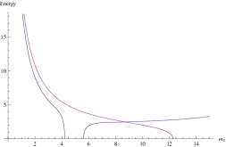
Figure 1: Graph of (60) with respect to $m_{2}$, for the red curve: $n=0,\alpha=2,\omega=3,\gamma=0.1,\beta=6$; for the blue curve: $n=3,\alpha=2,\omega=3,\gamma=0.1,\beta=6$

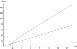
Figure 2: Graph of (86) with respect to $m_{2}$, for the red curve: $n=0,\omega=5,\alpha=1,\gamma=10,\delta=0.5;c=3$; for the blue curve: $n=3,\omega=5,\alpha=1,\gamma=10,\delta=0.5,c=3$

References

• [1] C.M. Bender and S. Boettcher, Phys. Rev. Lett. 80 5243 1998.
• [2] C.M. Bender, G.V. Dunne, P.N. Meisenger, Phys. Lett. A 252 272 1999; C.M. Bender and S. Boettcher J. Phys A: Math. Gen. 31, L273 1998; C. M. Bender, S. Boettcher, and V. M. Savage, J. Math. Phys. 41 6381 2000; C.M. Bender, D.C. Brody, H.F. Jones, Phys. Rev. Lett. 89 (2002) 270402; C.M. Bender, D.C. Brody, H.F. Jones, B.K. Meister, Phys. Rev. Lett. 98 (2007) 040403.
• [3] F. Cannata, G. Junker, J. Trost, Phys. Lett. A 246 219 1998; F. Cannata, M.V. Ioffe, D.N. Nishnianidze, Phys. Lett. A 310 344 2003; F. Cannata, J.P. Dedonder, A. Ventura, Ann. Phys. 322 397 2007.
• [4] M. Znojil, F. Cannata, B. Bagchi, R. Roychoudhury, Phys. Lett. B 483 284 2000; M. Znojil, J. Math. Phys. 46 062109 2005; M. Znojil, H.B. Geyer, Phys. Lett. B 640 52 2006.
• [5] G. LΓ©vai, M. Znojil, J. Phys. A: Math. Gen. 33 7165 2000;
• [6] B. Bagchi, C. Quesne, Phys. Lett. A 300 18 2002; B. Bagchi, S. Mallik C. Quesne, Mod. Phys. Lett. A 17 1651 2002; B. Bagchi, T. Tanaka, Phys. Lett. A 372 5390-5393 2008.
• [7] B. Bagchi, C. Quesne, Phys. Lett. A 273 285 2000; B. Bagchi, C. Quesne, J.Phys.A 43 305301 2010.
• [8] A. Mostafazadeh, J. Math. Phys. 43 205 2002; A. Mostafazadeh, J. Math. Phys. 43 2814 2002; A. Mostafazadeh, J. Math. Phys. 43 3944 2002; A. Mostafazadeh, J. Math. Phys. 45 932 2004;
• [9] B. Bagchi, C. Quesne, Phys. Lett. A 301 173 2002.
• [10] Z. Ahmed, Phys. Lett. A 294 287 2002.
• [11] F. Bagarello, M. Znojil, J. Phys. A: Math. Theor. 44 415305 2011; 45 115311 2012.
• [12] M. S. Swanson, J. Math. Phys. 45 585 2004.
• [13] L. Jin, Z. Song, Phys. Rev. A 84 042116.
• [14] I. O. Vakarchuk, J. Phys. A: Math. Gen. 38 4727 2005.
• [15] G. Soff, B. MΓΌller, J. Rafelski and W. Greiner, Z. Naturforsch A, 28 1389 1973.
• [16] C. Quesne and V. M. Tkachuk, J. Phys. A: Math. Gen. 37 4267 2004.
• [17] I. O. Vakarchuk, J. Phys. A: Math. Gen. 38 7567 2005.
• [18] C. Quesne and V. M. Tkachuk, J. Phys. A: Math. Gen. 38 1747 2005.
• [19] C.S Jia and A. de Souza Dutra, Ann. Phys. (NY) 323 566 2008.
• [20] C.S Jia and A. de Souza Dutra, J. Phys. A 39 11877 2006.
• [21] B. Bagchi and R. Roychoudhury, J. Phys. A 33 L1 2000.
• [22] O. Mustafa and S.H. Mazharimousavi, Int. J. Theor. Phys. 47 1112 2008.
• [23] L. B. Castro, Phys. Lett. A 375 2510 2011.
• [24] A. Sinha, P. Roy, Mod. Phys. Lett. A 20 2377 2005.
• [25] O. Mustafa, S. H. Mazharimousavi, J. Phys. A: Math. Gen. 40 863 2007.
• [26] O. Mustafa, S. H. Mazharimousavi, Int. J. Theor. Phys. 47 1112 2008.
• [27] A. Arda, R. Sever, Phys. Scr. 82(6) 065007 2010.
• [28] V.G.C.S. dos Santos, A. de Souza Dutra, M.B. Hott, Phys. Lett. A 373 3401 2009.
• [29] H. Eĝrifes, R. Sever, Phys. Lett. A 344 117 2005.
• [30] S. Longhi, Phys. Rev. Lett. 105 013903 2010.
• [31] A. Arda, R. Sever, Chin. Phys. Lett. 26, 090305 2009.
• [32] O. Mustafa, S. H. Mazharimousavi, Int. J. Theo. Phys. 47(4) 11 2006.
• [33] 1. Wen-Chao Qiang, Guo-Hua Sun, Shi-Hai Dong, Ann. Der Phy. 524 360 2012; P. K. Ghosh, Phys. Lett. A 375 3250 2011; M. V. Gorbatenko, V. P. Neznamov, Phys. Rev. D 83 105002 2011; R. Giachetti, V. Grecchi, J. Phys. A, 44 095308 2011; Xu-Yang Liu et al., Int. J. Theo. Phys. 49 343 2010; A. Szameit, et al, Phys. Rev. A 84 021806 2011; A. Arda, R. Sever, C. Tezcan, Chin. Phys. 27 010306 2010; O. Mustafa, Int. J. Theo. Phys. 47 1300 2008; O. Mustafa, M. Mazharimousavi, S. Habib, Int. J. Theo. Phys. 47 1112 2008.
• [34] B. P. Mandal, S. Gupta, Mod. Phys. Lett. A 25 1723 2010.
• [35] S. M. Ikhdair, J. Math. Phys. 51(2) 023525-1 2010.
• [36] H. Panahi and Z. Bakhshi, J. Phys. A: Math. Theo. 44 175304 2011.
• [37] E. Witten, Nucl. Phys. B 202 253 1982.
• [38] F. Cooper and B. Freedman, Ann. Phys. 146 262 1983.
• [39] L. E. Gendenshtein, JETP Lett. 38 356 1983.
• [40] L. Infeld and T. E. Hull, Rev. Mod. Phys. 23 21 1951.
• [41] J. Wu, Y. Alhassid, and F. GΓΌrsey, Ann. Phys. 196 163 1989.
• [42] A. Gangopadhyaya, J. V. Mallow, and U. P. Sukhatme, Phys. Rev. A 58 4287 1998.
• [43] C. Rasinariu, and U. Sukhatme, Phys. Lett. A 248 109 1998.
• [44] A. B. Balantekin, Phys. Rev. A 57 4188 1998.
• [45] G. LΓ©vai, J. Phys. A: Math. Gen. 22 689 1989.
• [46] F. Cooper, A. Khare U. Sukhatme, Supersymmetry in Quantum Mechanics, World Sci. Pub. Co. Pte. Ltd. 2001 ISBN: 981-02-4605-6.
• [47] A. D. Alhaidari, Phys. Lett. B 699(4) 309 2011.
• [48] H. Hassanabadi, S. Zarrinkamar, H. Rahimov, Commun. Theo. Phys. 56(3) 423 2011.
• [49] C. S. Jia, L. X. Ping, Z. L. Hui, Few-Body Sys. 52(1-2) 11 2012.
• [50] P. K. Ghosh, Phys. Lett. A 375 3250 2011.
• [51] G. A. Finney and J. Gea-Banacloche, Phys. Rev. E 54, 1449 1996.
• [52] L Sanz et al L Sanz et al, J. Phys. A: Math. Gen. 36 9737 2003.
• [53] Julia Diaz et al, Phys. Rev. A 86 023615 2012.
• [54] A. Sinha, P. Roy, J. Phys. A: Math. Theo. 41(33) 335306 2008; 42(5) 052002 2009; 40(34) 10599 2007.
• [55] H. F. Jones, J. Phys. A: Math. Theo. 42(13) 135303 2009.
• [56] B. Midya, P. P. Dube, R. Roychoudhury, J.of Phys. A: Math. and Theo. 44(6) 062001 2011.
• [57] P. E. G. Assis, J. Phys. A: Math. Theo. 44(26) 265303 2011.
• [58] Γ–. Yeşiltaş, J. Phys. A: Math. and Theo. 2011 44 305305.