Modeling the Lunar plasma wake

1 Introduction

Solar system bodies that lack a significant atmosphere and internal magnetic fields, such as the Moon and asteroids, can to a first approximation be considered passive absorbers of the solar wind. The solar wind ions and electrons directly impact the surface of these bodies, and a wake is created behind the object. In a frame that moves with the solar wind plasma, the refill of the lunar wake can be viewed as the more general problem of plasma expansion into a vacuum.

One-dimensional plasma expansion into a vacuum has been studied for a long time, see [1] and references therein. The specific case of one-dimensional plasma expansion into the lunar wake has also been studied [2, 3]. A disadvantage of one-dimensional models is that the magnetic field component along the dimension is forced to be constant, from the requirement that $\nabla\cdot\mathbf{B}=0$. On the other hand, three dimensional models [4] does not allow the same spatial resolution and size of the simulation domain as lower dimensional models, due to computational constraints. Thus, a two-dimensional model of the lunar wake refill could be useful.

A one-dimensional approximation of the lunar wake is an initial state with uniform plasma, corresponding to the solar wind, surrounding a region of vacuum (zero density) of width equal to the lunar radius. With time the plasma will expand into the vacuum region. This approximates plasma conditions along a line that at $t=0$ lies in the terminator plane and goes through the center of the Moon. The line then convects with the solar wind as time goes by. The magnetic field at $t=0$ corresponds to the interplanetary magnetic field (IMF) in the solar wind. It is possible to use the same convecting frame approach also in two dimensions. If we consider the terminator plane at $t=0$ and let this plane convect with the solar wind plasma bulk velocity, $u_{sw}$, it will at time $t$ be at $x=-tu_{sw}$. The initial configuration at $t=0$ is the $yz$-plane with proton number density $n=n_{0}$ for $r<R$, and $n=n_{sw}$ for $r>R$. Here the $x$-axis is anti-parallel to the solar wind, and $r=\sqrt{y^{2}+z^{2}}$. We study such plasma expansion into a vacuum in a two-dimensional geometry using a hybrid model with $R=1730$ km. The hybrid model has ions as particles and electrons as a mass-less fluid, and is described in [4], and references therein. In the hybrid model the electric field computation involves a division by charge density. Thus, there is a problem in vacuum regions. Here we handle this by letting $n_{0}$ have a small, non-zero value. In this case $n_{0}=0.1n_{sw}$. However, this low density population of ions is not shown in the plots.

We can note that more complicated low dimensional models are possible. We could follow the convecting plane (or line in the one-dimensional case) from upstream, in the undisturbed solar wind, and after each time step remove ions that collide with the Lunar surface from the ion velocity space distribution. This removal would continue until the plane has convected past the Moon. The solution would however no more be independent on the solar wind velocity.

2 Results

In what follows, the solar wind number density, $n_{sw}=5$ cm^-3, the ion temperature is $5\cdot 10^{4}$ K, the electron temperature is $10\cdot 10^{4}$ K, and the IMF is in the $xy$-plane with a magnitude of 5 nT. For these plasma parameters, the ion inertial length is 100 km, the Alfvén velocity is 49 km/s, the thermal proton gyro radius is 60 km (the gyro time is 13 s), and the ion plasma beta is 0.35. The cell size is 78 km and the number of meta particles per cell is 170.

How the wake number density depends on the direction of the initial magnetic field is shown in Fig. 1.

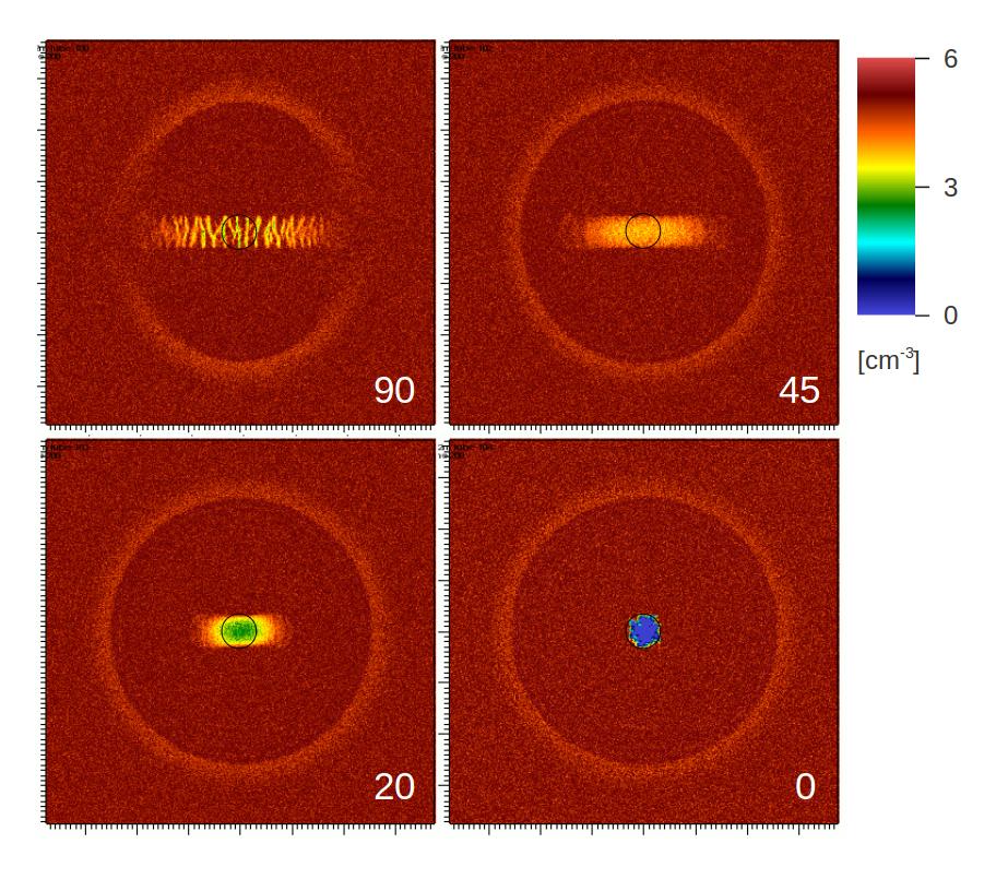
Figure 1: Proton number density in the $yz$-plane at $t=200$ s for an IMF direction of 90, 45, 20, and 0 degrees away from the image normal (solar wind direction). The plane of the IMF is horizontal. The black circle show the outline of the initial low density region of radius 1730 km (representing the Moon).

The time $t=200$ s of the plot corresponds to a distance of $tu_{sw}$ downstream of the moon, e.g., for $u_{sw}=500$ km/s the distance is 10,000 km $\approx$ 5.8 Lunar radii.

We see a density rarefaction that expands from the Moon at the fast magnetosonic speed, as has been seen before in three-dimensional simulations [4]. It does not propagate parallel to the IMF as can be seen for the case of an IMF at a 90 deg angle to the solar wind flow direction. At this time, for these condition, the wake has partially refilled except for the case of a 0 deg IMF (parallel to the solar wind flow) for which we still have a (deformed) vacuum region. We also see that the wake is flattened in the plane of the IMF due to the fact that the ions flow along the IMF.

For the 90 deg IMF case we see density oscillations in the refilled region, where surrounding plasma intrudes. In the next section we derive criteria for an instability in the hybrid model that can be a possible cause for these oscillations. Note that these oscillations are a feature of the hybrid model, it is unknown if such oscillations also would occur in a 2D particle in cell model of the Lunar wake that includes also electrons as particle.

3 Ion beam instability in a hybrid model

For longitudal waves propagating along the magnetic field lines, the hybrid model reads

$$\frac{\partial f_{i}}{\partial t}+v\frac{\partial f_{i}}{\partial x}+\frac{eE}{m_{i}}\frac{\partial f_{i}}{\partial v}=0$$ (1)

where the electric field is obtained from the electron momentum equation as

$$E=\frac{k_{B}T_{e}}{e}\frac{\partial}{\partial x}\bigg{(}\frac{n}{n_{0}}\bigg{)}^{5/3},$$ (2)

and quasi-neutrality gives

$$n=\int f_{i}d^{3}v$$ (3)

Linearization $f_{i}=f_{0}+f_{1}$, $E=E_{1}$, $n=n_{0}+n_{1}$ gives

$$\frac{\partial f_{1}}{\partial t}+v\frac{\partial f_{1}}{\partial x}+\frac{eE_{1}}{m_{i}}\frac{\partial f_{0}}{\partial v}=0$$ (4)

$$E_{1}=\frac{5}{3}\frac{k_{B}T_{e}}{en_{0}}\frac{\partial n_{1}}{\partial x},$$ (5)

and

$$n_{1}=\int f_{1}d^{3}v$$ (6)

Laplace transformation $\partial/\partial t\rightarrow-i\omega$ and $\partial/\partial x\rightarrow ik$ gives

$$(-i\omega+ivk)f_{1}+\frac{eE_{1}}{m_{i}}\frac{\partial f_{0}}{\partial v}=0,$$ (7)

and

$$E_{1}=\frac{5}{3}\frac{k_{B}T_{e}}{en_{0}}ikn_{1}=\frac{5}{3}\frac{k_{B}T_{e}}{en_{0}}ik\int f_{1}d^{3}v=-\frac{5}{3}\frac{k_{B}T_{e}}{m_{i}n_{0}}ikE_{1}\int\frac{1}{-i\omega+ivk}\frac{\partial f_{0}}{\partial v}d^{3}v.$$ (8)

Eliminating the common factor $E_{1}$ and rearranging the terms, we obtain the dispersion relation

$$1+\frac{5}{3}\frac{k_{B}T_{e}}{m_{i}n_{0}}\int\frac{1}{v-\omega/k}\frac{\partial f_{0}}{\partial v}d^{3}v=0,$$ (9)

Here the frequency and wavenumber appear only as a ratio $\omega/k$. If we replace this ratio by $v_{p}$, the ”phase velocity”, we obtain the equation

$$1+\frac{5}{3}\frac{k_{B}T_{e}}{m_{i}n_{0}}\int\frac{1}{v-v_{p}}\frac{\partial f_{0}}{\partial v}d^{3}v=0,$$ (10)

Note that in this equation, $v_{p}$ depends only on the plasma parameters but not on $\omega$ or $k$. Hence $v_{p}$ is a complex number, $v_{p}=v_{R}+iv_{I}$, which can either have positive or negative imaginary parts $v_{I}$. The dispersion relation can be written $\omega=(v_{R}+iv_{I})k$. If $v_{I}$ is positive, then we have an instability which formally goes to infinity as $k\rightarrow\infty$. In a simulation, however, the wavenumber is limited by the grid size.

4 Acknowledgments

This work was supported by the Swedish National Space Board, and the Swedish National Infrastructure for Computing. The software used in this work was in part developed by the DOE NNSA-ASC OASCR Flash Center at the University of Chicago.

References

- [1] P. Mora, Phys. Rev. Lett. 90, 185002 (2003)
- [2] W.M. Farrell et al., J. Geophys. Res. 103, 23653–23660 (1998)
- [3] P.C. Birch, and S.C. Chapman, Physics of Plasmas 8, 4551–4559 (2001)
- [4] M. Holmström et al., Earth Planets Space, 64, 237–245 (2012)