Spin-dipole strength functions of ⁴He with realistic nuclear forces

Abstract

Both isoscalar and isovector spin-dipole excitations of ⁴He are studied using realistic nuclear forces in the complex scaling method. The ground state of ⁴He and discretized continuum states with $J^{\pi}=0^{-},\,1^{-},\,2^{-}$ for $A=4$ nuclei are described in explicitly correlated Gaussians reinforced with global vectors for angular motion. Two- and three-body decay channels are specifically treated to take into account final state interactions. The observed resonance energies and widths of the negative-parity levels are all in fair agreement with those calculated from both the spin-dipole and electric-dipole strength functions as well as the energy eigenvalues of the complex scaled Hamiltonian. Spin-dipole sum rules, both non energy-weighted and energy-weighted, are discussed in relation to tensor correlations in the ground state of ⁴He.

I Introduction

Spin-dipole (SD) excitations of nuclei have attracted much attention because of their connection with, for example, tensor correlation, neutron skin-thickness and neutrino-nucleus scattering. Especially the neutrino reaction involving light nuclei is important to the nucleosynthesis at various stages. In the final stage of a core collapse supernova, the nuclei are exposed to the intense flux of neutrinos, and the neutrino-nucleus reaction rate is determined by the nuclear responses to such operators of the weak interaction as Gamow-Teller (GT), dipole, SD, and so on gazit07 ; tsuzuki06 . The SD operator brings about the first-forbidden transition of the weak interaction. In the case of $N=Z$ nuclei, the allowed transition probability due to the weak interaction is small, and thus the first-forbidden transition can be a leading order, making a primary contribution to the cross section.

Though the neutrino-nucleus reaction cross section can not be measured to good accuracy in a laboratory because of its too small reaction rate, information on the spin excitation of nuclei can be obtained using a charge-exchange reaction. For example, in the $(p,n)$ or $(d,^{2}$He$)$ reaction at intermediate energy, the cross section at 0 degree is a useful probe to extract the GT strength fujita11 as well as the SD strength okamura02 ; huu07 . The SD excitation can be obtained by measuring the cross section at larger angles gaarde84 ; rapaport94 . For a doubly closed shell nucleus the SD contribution is fairly large even at 0 degree because of the hindrance of the GT strength. Much effort has been devoted to measure the SD transitions in light nuclei. Recently the charge-exchange reaction of (⁷Li,⁷Be$\gamma$) is undertaken to measure the electric dipole $(E1)$ and the SD resonances of ⁴He and ^6,7Li nakayama07 ; nakayama08 . A more recent measurement of polarization transfer observables with ¹⁶O$(\vec{p},\vec{n})^{16}$F reaction wakasa11 indicates that valuable information on the SD excitations is attainable.

The SD transition is also interesting in comparison with the $E1$ transition. The SD operator can change the spin wave function of the ground state, whereas the $E1$ operator can not. Since the SD operator has three possible multipoles, the study of its transition strength is expected to be more advantageous to see the spin structure of nuclei than that by the $E1$ operator dumitrescu84 . That is, this multipole dependence of the SD operator may be used to probe the role of non-central forces, especially the tensor force. The effect of the tensor force has in fact been studied theoretically by looking at the SD excitations in the shell model tsuzuki98 and in the random phase approximation based on Skyrme-Hartree-Fock bai10 ; bai11 and relativistic Hartree-Fock methods liang12 . All these calculations employed the variety of effective interactions and found that the residual tensor terms added to the interaction play some multipole-dependent effects on the SD strength functions.

The purpose of this paper is to study the SD excitations of ⁴He using realistic nucleon-nucleon interactions. Only the ground state of ⁴He is bound among $A=4$ nucleon systems and its basic property is now understood fairly well thanks to several accurate methods for solving bound state problems of few-body systems kamada01 . All the excited states of ⁴He are in continuum and its negative-parity states below the $2n+2p$ threshold have $J=0,1,2$ with $T=0$ and 1. These resonances as well as the continuum states may be reached by the SD operators. It is therefore quite challenging to accurately predict the SD strength function as a function of excitation energy because we have to deal with the continuum states where not only two but also three particles may play an important contribution. On top of that we have to take into account both short-range and tensor correlations due to the realistic nuclear forces forest96 ; feldmeier11 . Very recently the present authors and Arai have done an ab initio calculation for the photoabsorption of ⁴He horiuchi12a using square integrable ($\mathcal{L}^{2}$) basis functions in the framework of the complex scaling method (CSM) and have reproduced most of experimental photoabsorption cross section data up to the pion threshold. A theoretical approach employed in the present paper is similar to that of the $E1$ case.

It is well known that the ground state of ⁴He contains the $D$-state (or the total spin $S=2$ state) probability by about 14%, which is of course due to the tensor force. As shown in the calculation of bound-state approximation horiuchi08 ; horiuchi12b , the tensor force plays a vital role in correctly reproducing the spectrum of the excited states of ⁴He. If one uses such effective interactions that contain no tensor components, there is no way to account for the level splittings of the negative-parity states of ⁴He. Therefore the use of realistic nuclear forces is absolutely necessary for studying the SD strength in ⁴He. In the same context we also study the charge-exchange SD transitions from ⁴He, leading to the negative-parity states of ⁴H or ⁴Li. We will pay due attention to the effect of the tensor correlation on the SD excitations. It should be noted that the SD excitation is here described based on the accurate ground-state wave function of ⁴He horiuchi08 ; horiuchi12b . We also note that this study will serve fundamental data on the neutrino-⁴He reaction cross section in stars by integrating the SD strength functions weighted by the neutrino energy distribution produced by the core collapse star.

In Sec. II we present our method of evaluating the SD strength functions, the CSM (Sec. II.1) and the $\mathcal{L}^{2}$ basis functions (Sec. II.2) that are keys in the present calculation. We show calculated results on the SD strength functions in Sec. III. The SD strengths calculated from continuum-discretized states are presented in Sec. III.1. The SD strength functions of both isovector and isoscalar types are displayed in Sec. III.2. A comparison of the peaks of the SD strength functions with the resonance properties of ⁴He is made in Sec. III.3. The SD sum rules, both non energy-weighted and energy-weighted, are discussed in Sec. III.4. Conclusions are drawn in Sec. IV. A multipole decomposition of the SD non energy-weighted sum rule (NEWSR) is discussed in Appendix A, and a method of calculating its relevant matrix element with our basis functions is briefly explained in Appendix B. In Appendix C we derive a formula that makes it possible to calculate the contribution of the kinetic energy operator to the SD energy-weighted sum rule (EWSR).

II Calculation method of spin-dipole strength function

II.1 Complex scaling method

The SD operator with the multipolarity $\lambda$ and its projection $\mu$ is defined by

$$\mathcal{O}_{\lambda\mu}^{p}=\sum_{i=1}^{N}\left[\bm{\rho}_{i}\times\bm{\sigma}_{i}\right]_{\lambda\mu}T^{p}_{i}$$ (1)

with

$$\bm{\rho}_{i}=\bm{r}_{i}-\bm{x}_{N},$$ (2)

where $\bm{r}_{i}$ is $i$th nucleon coordinate, $\bm{x}_{N}$ is the center-of-mass coordinate of the ${N}$-nucleon system, and $\bm{\sigma}_{i}$ is $i$th nucleon spin. The center-of-mass motion is completely removed in the present paper and only the intrinsic excitation is considered. The square bracket $[\bm{\rho}_{i}\times\bm{\sigma}_{i}]_{\lambda\mu}$ denotes the angular momentum coupling of the two vectors or more generally the tensor product of spherical tensors to that operator specified by $\lambda\,\mu$. The value of $\lambda$ can take 0, 1, and 2. The superscript $p$ of $\mathcal{O}_{\lambda\mu}^{p}$ or $T^{p}_{i}$ distinguishes different types of isospin operators, isoscalar (IS), isovector (IV0), and charge-exchange (IV$+$ and IV$-$), that is,

$$T^{\rm IS}_{i}=1,\quad T^{\rm IV0}_{i}=\tau_{z}(i),\quad T^{\rm IV\pm}_{i}=t_{\pm}(i).$$ (3)

In the inelastic neutrino-nucleus reaction, the neutral current induces the IV0 type operator as well as the IS one. The isospin operator $t_{+}=t_{x}+it_{y}$ $(t_{-}=t_{x}-it_{y})$ converts a proton (neutron) to a neutron (proton), which corresponds to the charge-exchange process $X(n,p)Y$ $(X(p,n)Y)$.

The strength function of an initial state $\Psi_{0}$ for the SD operator is defined as

$$S(p,\lambda,E)=\mathcal{S}_{f\mu}|\left<\Psi_{f}\right|\mathcal{O}^{p}_{\lambda\mu}\left|\Psi_{0}\right>|^{2}\delta(E_{f}-E_{0}-E)$$

$$=-\frac{1}{\pi}\text{Im}\sum_{\mu}\left<\Psi_{0}\right|\mathcal{O}^{p\dagger}_{\lambda\mu}\frac{1}{E+E_{0}-H+i\epsilon}\mathcal{O}^{p}_{\lambda\mu}\left|\Psi_{0}\right>,$$ (4)

where $\mathcal{S}_{f\mu}$ represents a summation over $\mu$ and all the final states $\Psi_{f}$. Both the initial and final states are the eigenfunctions of a Hamiltonian $H$ with the energies $E_{0}$ and $E_{f}$. They are normalized as usual: $\left<\Psi_{\nu^{\prime}}|\Psi_{\nu}\right>=\delta_{\nu^{\prime}\nu}$ and $\delta(E_{\nu^{\prime}}-E_{\nu})$ for bound and unbound states, respectively. In the second expression of Eq. (4) the summation over the final states with the energy conservation of $\delta(E_{f}-E_{0}-E)$ is converted to the imaginary part of a resolvent $R$

$$R=\frac{1}{E+E_{0}-H+i\epsilon}.$$ (5)

In the present paper we use the CSM to obtain the strength function. The CSM is widely used not only in atomic and molecular physics ho83 ; moiseyev98 but in nuclear physics CSM as well. Very recently it has successfully been applied to calculate the photoabsorption cross section of ⁴He with a realistic Hamiltonian horiuchi12a . The CSM allows us to obtain the strength function using only $\mathcal{L}^{2}$ basis functions exclusively, making it possible to avoid an explicit construction of the continuum state. The key of the CSM is to rotate both the coordinate and the momentum by a scaling angle $\theta$

$$\bm{r}_{j}\to\bm{r}_{j}e^{i\theta},\quad\bm{p}_{j}\to\bm{p}_{j}e^{-i\theta},$$ (6)

which makes the continuum state damp at large distances within a certain range of $\theta$. The strength function $S(p,\lambda,E)$ reduces to

$$S(p,\lambda,E)$$

$$=-\frac{1}{\pi}\text{Im}\sum_{\mu}\left<\Psi_{0}\right|\mathcal{O}_{\lambda\mu}^{p\dagger}U^{-1}(\theta)R(\theta)U(\theta)\mathcal{O}^{p}_{\lambda\mu}\left|\Psi_{0}\right>,$$ (7)

where $U(\theta)$ is the scaling operator that makes the transformation (6) and $R(\theta)$ is the complex scaled resolvent

$$R(\theta)=U(\theta)RU^{-1}(\theta)=\frac{1}{E+E_{0}-H(\theta)+i\epsilon}$$ (8)

with the rotated Hamiltonian

$$H(\theta)=U(\theta)HU^{-1}(\theta).$$ (9)

Provided the eigenfunctions of $H(\theta)$ are made to damp at large distances, they can be expanded with a set of $\mathcal{L}^{2}$ basis functions $\Phi_{i}(\bm{x})$

$$\Psi_{\nu}(\theta)=\sum_{i}C_{i}^{\nu}(\theta)\Phi_{i}(\bm{x}).$$ (10)

The coefficients $C_{i}^{\nu}(\theta)$ together with the complex eigenvalue $E_{\nu}(\theta)$ are determined by diagonalizing $H(\theta)$:

$$H(\theta)\Psi_{\nu}(\theta)=E_{\nu}(\theta)\Psi_{\nu}(\theta).$$ (11)

The strength function $S(p,\lambda,E)$ is then calculated from the following expression:

$$S(p,\lambda,E)=-\frac{1}{\pi}\sum_{\nu,\mu}\text{Im}\frac{\tilde{\mathcal{D}}^{p,\nu}_{\lambda\mu}(\theta)\mathcal{D}^{p,\nu}_{\lambda\mu}(\theta)}{E+E_{0}-E_{\nu}(\theta)+i\epsilon},$$ (12)

where

$$\mathcal{D}^{p,\nu}_{\lambda\mu}(\theta)=\left<(\Psi_{\nu}(\theta))^{*}\right|\mathcal{O}^{p}_{\lambda\mu}(\theta)\left|U(\theta)\Psi_{0}\right>,$$

$$\mathcal{\tilde{D}}_{\lambda\mu}^{p,\nu}(\theta)=\left<(U(\theta)\Psi_{0})^{*}\right|\tilde{\mathcal{O}}^{p}_{\lambda\mu}(\theta)\left|\Psi_{\nu}(\theta)\right>$$ (13)

with

$$\mathcal{O}_{\lambda\mu}^{p}(\theta)=\mathcal{O}_{\lambda\mu}^{p}e^{i\theta},\quad\tilde{\mathcal{O}}_{\lambda\mu}^{p}(\theta)=\mathcal{O}_{\lambda\mu}^{p\dagger}e^{i\theta}.$$ (14)

Note that $U(\theta)\Psi_{0}$ is here taken to be the solution of Eq. (11) corresponding to the initial state.

If a sharp resonance exists, the angle $\theta$ has to be rotated to cover its resonance pole on the complex energy plane moiseyev98 ; CSM . Practically the scaling angle $\theta$ is chosen by examining the stability of the strength function with respect to $\theta$. See Refs. horiuchi12a ; horiuchi12b for some examples on the $\theta$-dependence.

II.2 Correlated Gaussians and global vectors

II.2.1 Hamiltonian

The Hamiltonian $H$ we use contains two- and three-nucleon interactions

$$H=\sum_{i=1}^{N}T_{i}-T_{\text{cm}}+\sum_{i<j}v_{ij}+\sum_{i<j<k}v_{ijk}.$$ (15)

In the kinetic energy $T_{i}$ the proton-neutron mass difference is ignored. Two different two-nucleon interactions, AV8^′ AV8p and G3RS G3RS potentials, are employed to examine the extent to which the strength function is sensitive to the $D$-state probability of ⁴He. The $\bm{L}^{2}$ and $(\bm{L}\cdot\bm{S})^{2}$ terms in the G3RS potential are ignored. The AV8^′ potential is more repulsive at short distances and has a stronger tensor component than the G3RS potential. As the three-body interaction (3NF) we adopt the spin-isospin independent phenomenological potential hiyama04 that is adjusted to reproduce both the inelastic electron scattering form factor to the first excited state of ⁴He as well as the binding energies of ^3,4He and ³H. The Coulomb potential is included, but the isospin is treated as a conserved quantum number. The nucleon mass $m_{N}$ and the charge constant $e$ used in what follows are $\hbar^{2}/m_{N}=41.47106$ MeV fm² and $e^{2}=1.440$ MeV fm.

II.2.2 Basis functions for bound states

We solve the four-body Schrödinger equation using a variational method. A choice of the variational trial functions is essential to determine the accuracy of the calculation. A bound-state solution with spin-parity $J^{\pi}$ of $N$-nucleon system may be expressed in terms of a linear combination of the $LS$ coupled basis functions

$$\Phi_{(LS)JM_{J}TM_{T}}^{\pi}=\mathcal{A}\left[\phi_{L}^{\pi}\times\chi_{S}\right]_{JM_{J}}\eta_{TM_{T}},$$ (16)

where $\mathcal{A}$ is the antisymmetrizer, and the spin function $\chi_{S}$ is given in a successive coupling as

$$\chi_{S_{12},S_{123},\dots,SM_{S}}$$

$$=[\dots[[\chi_{\frac{1}{2}}(1)\times\chi_{\frac{1}{2}}(2)]_{S_{12}}\times\chi_{\frac{1}{2}}(3)]_{S_{123}}\dots]_{SM_{S}}.$$ (17)

Note that the above spin function forms a complete set provided all possible intermediate spins ($S_{12},S_{123}$, $\dots$) are included for a given $S$. The isospin function $\eta_{TM_{T}}$ is given in exactly the same way as the spin function.

The spatial part $\phi_{L}^{\pi}$ should be flexible enough to cope with the strong tensor force and short-range repulsion. The tensor force mixes the $S$ and $D$ components in the wave function and the short-range repulsion makes the amplitude of the two-nucleon relative motion function vanishingly small at short distances. Many examples show that the correlated Gaussian (CG) basis boys60 ; singer60 is flexible enough to meet these requirements  varga97 ; kamada01 ; horiuchi08 . See a recent review mitroy13 for various powerful applications of the CG. Let an $(N-1)$-dimensional column vector or an $(N-1)\times 1$ matrix $\bm{x}$ denote a set of relative coordinates whose $i$th element is a 3-dimensional vector $\bm{x}_{i}$. A set of the Jacobi coordinates is most often employed for $\bm{x}$ but other sets of relative coordinates may be used as well. The spatial part $\phi_{L}^{\pi}$, given in the CG with two global vectors (GV), takes a form varga95 ; svm ; suzuki08 ; aoyama12

$$F_{(L_{1}L_{2})LM_{L}}(u_{1},u_{2},A,\bm{x})$$

$$=\exp(-\textstyle{\frac{1}{2}}\tilde{\bm{x}}A\bm{x})\left[\mathcal{Y}_{L_{1}}(\tilde{u}_{1}\bm{x})\times\mathcal{Y}_{L_{2}}(\tilde{u}_{2}\bm{x})\right]_{LM_{L}}$$ (18)

with

$$\mathcal{Y}_{\ell m}(\bm{v})=v^{\ell}Y_{\ell m}(\hat{\bm{v}}),$$ (19)

where $A$ is an $(N-1)\times(N-1)$ positive-definite, symmetric matrix and $\tilde{\bm{x}}A\bm{x}$ is a short-hand notation for $\sum_{i,j=1}^{N-1}A_{ij}\bm{x}_{i}\cdot\bm{x}_{j}$. The tilde stands for the transpose of a matrix. Parameters $u_{1}$ and $u_{2}$ are $(N-1)$-dimensional column vectors that define the GVs, $\tilde{u}_{1}\bm{x}(=\sum_{i=1}^{N-1}{u_{1}}_{i}\bm{x}_{i})$ and $\tilde{u}_{2}\bm{x}$, and these characterize the angular motion of the system.

The CG-GV basis (18) apparently describes correlated motion among the particles through the off-diagonal elements of $A$ and the rotational motion of the system is conveniently described by different sets of $(L_{1},L_{2})$ carried by the two GVs. Most noticeable among several advantages of the CG-GV basis functions are that the functional form of Eq. (18) remains unchanged under an arbitrary linear transformation of the coordinate $\bm{x}$, that the matrix elements for most operators can be evaluated analytically, and that the formulation can readily be extended to systems with larger $N$. Useful formulas for evaluating matrix elements with the CG-GV basis are collected in Appendices of Refs. suzuki08 ; aoyama12 .

All possible $L,\,S$ sets are adopted to specify the basis functions for a given $J$. The value of $S$ can be 0, 1, and 2 for the four-nucleon system, and all possible $L$ values that make $J$ with $S$ are included. For a given $L^{\pi}$ we choose the simplest combination of ($L_{1}$,  $L_{2}$): ($L_{1}=L,\,L_{2}=0$) for a natural parity state with $\pi=(-1)^{L}$ and $(L_{1}=L,\,L_{2}=1$) for an unnatural parity state with $\pi=(-1)^{L+1}$, respectively. An exception is that no basis function with $L^{\pi}=0^{-}$ is included in our calculation because that special case needs at least three GVs suzuki00 ; aoyama12 . It should be noted, however, that the $L^{\pi}=0^{-}$ configuration may be excited by the $E1$ and SD transitions only through the $(L=S=1)$ component of the ground state of ⁴He. Since the probability of finding that component is quite small (less than 0.4%) kamada01 ; suzuki08 , practically we do not miss any SD strength by the neglect of the $L^{\pi}=0^{-}$ configuration. This is really the case in the $E1$ strength function horiuchi12a and in the SD case as well as shown in Sec. III.4.

The parameters, $A$, $u_{1}$, and $u_{2}$, are determined by the stochastic variational method (SVM) varga94 ; varga95 ; svm . The calculated properties of ³H, ³He, and ⁴He agree with experimental three- and four-nucleon data very well horiuchi12b .

II.2.3 Square-integrable basis functions for spin-dipole excitations

We construct the basis functions for the final states with $J^{-}T$ that are excited by the SD operator $\mathcal{O}_{\lambda\mu}^{p}$ of $\lambda=J$. The accuracy of the CSM calculation depends on how fully the basis functions are prepared. In Ref. horiuchi12a , the present authors and Arai described a way to construct the four-body continuum-discretized states with $J^{\pi}T=1^{-}1$. The guidelines of the construction were to take into account both sum rule and final state interactions between the particles in the continuum. The total photoabsorption cross section is calculated via the $E1$ strength function and it succeeds to reproduce the measured cross section up to the pion threshold. Here we take the same route as that of Ref. horiuchi12a with a possible modification due to the spin flip of the SD operator.

We define a single-particle (sp) basis, which describes a single-particle like excitation from the correlated ground state by the SD operator. This class of basis functions is expected to play a vital role in accounting for all the SD strength. The basis is constructed as

$$\Psi_{f}^{\text{sp}}=\mathcal{A}\left[\left[\phi_{L_{i}}^{+}(i)\times\chi_{S^{\prime}}\right]_{J^{\prime}}\times\mathcal{Y}_{1}({\bm{\rho}}_{1})\right]_{\lambda\mu}\eta_{TM_{T}},$$ (20)

where $\phi_{L_{i}}^{+}(i)$ is the space part of the $i$th basis function of a truncated ground-state wave function, $\Psi_{0000}^{+}$, of ⁴He. The wave function $\Psi_{0000}^{+}$ consists of $[\phi_{0}^{+}\times\chi_{0}]_{00}\eta_{00}$ and $[\phi_{2}^{+}\times\chi_{2}]_{00}\eta_{00}$, with any configurations of $[\phi_{1}^{+}\times\chi_{1}]_{00}\eta_{00}$ being omitted, which leads to 1.53 MeV loss for the ground-state energy of ⁴He. See Ref. horiuchi12a for the detail. As for the spin part, differently from the $E1$ case horiuchi12a we take into account the complete set for a given $S^{\prime}$, which, depending on the total spin $S_{i}$ of the $i$th basis function of $\Psi_{0000}^{+}$, is chosen as $S^{\prime}=1$ for $S_{i}=0$ and $S^{\prime}=1$ and 2 for $S_{i}=2$, respectively.

The $3N+N$ two-body and $d+p+n$ three-body disintegration channels are defined in the same manner as in Ref. horiuchi12a .

The calculations are performed not only in each basis set of sp, $3N+N$ and $d+p+n$ but also in the ‘Full’ basis that includes all of them. The number of basis functions in the Full model with the AV8^′+3NF potential is 2980, 6400, 6540, 4380, 8800, 9540 for $J^{\pi}T=0^{-}0,1^{-}0,2^{-}0,0^{-}1,1^{-}1,2^{-}1$, respectively.

III Results and discussions

III.1 Discretized spin-dipole strength

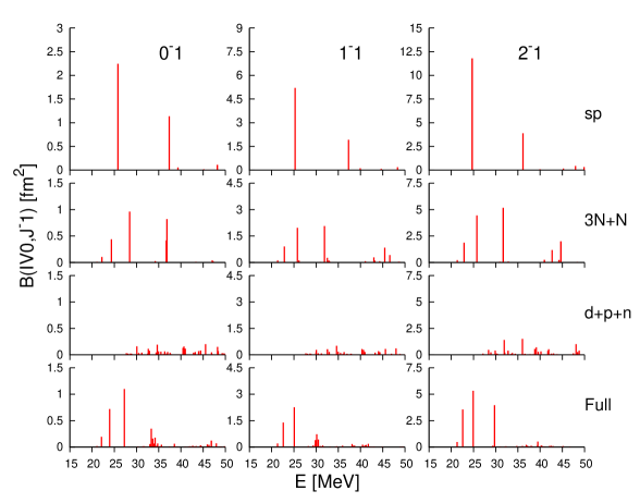
Figure 1: (Color online) The discretized isovector SD reduced transition probabilities of IV0 type for ⁴He as a function of excitation energy. The $J^{\pi}T$ values of the excited states are $0^{-}1,1^{-}1,$ and $2^{-}1$, respectively. The transition probabilities are displayed, arranged vertically for each $J^{\pi}T$ case, depending on the configurations included in the calculation. See text for details. The AV8^′+3NF interaction is used.

First we show the continuum-discretized SD strength. For this purpose the Hamiltonian is diagonalized in the basis states that are defined in Sec. II.2.3. This calculation corresponds to the CSM solution with $\theta=0^{\circ}$. Figure 1 displays the reduced transition probability for the IV SD operator ($p={\rm IV0}$)

$$B(p,J^{-}T,\nu)=\sum_{M\mu}\left|\right<\Psi^{J^{-}MT}_{\nu}(\theta=0^{\circ})|\mathcal{O}_{\lambda\mu}^{p}|\Psi_{0}\left>\right|^{2},$$ (21)

as a function of the discretized energy $E_{\nu}(\theta=0^{\circ})$, where $\nu$ is the label to distinguish the discretized energy. Here $\lambda$ is equal to $J$ and $T=1$.

The results of calculation are similar to the $E1$ case of Ref. horiuchi12a . In the calculation with the sp configuration only, the strength is concentrated at one state that appears at about 25 MeV for all the cases with $J^{\pi}T=0^{-}1,\,1^{-}1,\,2^{-}1$. The state may correspond to the observed level at 23.33 MeV for $J^{\pi}T=2^{-}1$ and 25.28 MeV for $J^{\pi}T=0^{-}1$, respectively tilley92 . For the $J^{\pi}T=1^{-}1$ case, two levels with very broad widths are known at 23.64 and 25.95 MeV. Since the energy of the prominent SD transition strength is lower than that obtained for the $E1$ transition strength horiuchi12a , the 23.64 MeV level probably has SD character, whereas the 25.95 MeV level is excited by the $E1$ operator.

Similarly to the $E1$ transition strength horiuchi12a , two or three peaks are obtained with the $3N+N$ configuration and relatively small strength is spread broadly above 30 MeV. The prominent peaks below 30 MeV shown in the $3N+N$ calculation continue to remain in the Full basis calculation, which again confirms the importance of the $3N+N$ configuration to describe the low-energy SD strengths as in the $E1$ strength. We also calculate the SD strength with the G3RS+3NF interaction. Both distributions look similar, indicating the weak dependence of the SD strength on the realistic interactions employed.

The so-called softening and hardening of the SD excitation is discussed in Refs. bai10 ; bai11 , where the residual tensor force is turned on or off and the energy and the strength of the SD excitation are compared each other. We think that the conclusion drawn by such comparisons is not always true because switching off the important piece of the nucleon-nucleon interaction may cause a significant change in the continuum structure that can be reached by the SD operator. In fact, we can not turn off the tensor force. If the tensor force were switched off, the ground state of ⁴He would not be bound and moreover the spectrum of the negative-parity states would be far from the observed one horiuchi08 ; horiuchi12b . As will be discussed later, we find no quenching of the SD strength but confirm that our SD strength calculated with the realistic nuclear forces satisfies the NEWSR perfectly.

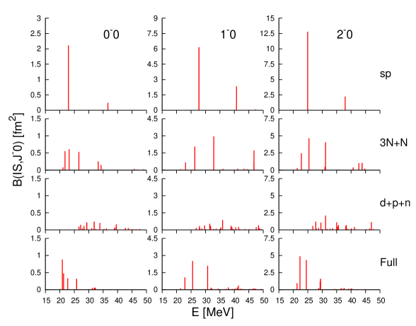
Figure 2: (Color online) The same as Fig. 1 but for the isoscalar SD transitions. The $J^{\pi}T$ values of the excited states are $0^{-}0,1^{-}0,$ and $2^{-}0$, respectively.

Figure 2 displays the reduced transition probability for the IS SD operator ($p={\rm IS}$). The gross structure of the strength is similar to the IV SD case. In the sp configuration calculation, strongly concentrated peaks appear at the energies not far from the observed levels tilley92 : 21.01, 21.84, 24.25 MeV for $J^{\pi}T=0^{-}0,2^{-}0,1^{-}0$, respectively. The importance of the $3N+N$ configurations is indicated by those peaks that appear in the $3N+N$ configuration calculation and continue to exist in the Full calculation. The Full calculation predicts one prominent peak at 20.85 MeV for $J^{\pi}T=0^{-}0$, which may correspond to the 21.01 MeV level with the small decay width of $0.84$ MeV tilley92 . In the case of $J^{\pi}T=2^{-}0$, the two prominent strengths are obtained at the energies close to each other, suggesting a relatively small decay width. The relationship between the strength functions and resonance properties will be discussed in Sec. III.3.

Three negative-parity states of ⁴He with $J=0,\,1,\,2$ and $T=0$ are observed slightly above the $2n+2p$ threshold of 28.3 MeV tilley92 . These states may be excited by the IS SD operator. In fact, a comparison of the IS and IV SD strengths obtained in the $d+p+n$ configurations clearly suggests that more strength is found in the IS case around the excitation energy of 30 MeV. Therefore some discretized states at around 30 MeV shown in Fig. 2 may be precursors of those observed states. Since the three observed states almost entirely decay by emitting deuterons, it is likely that they have $d+d$ structure with a $P$-wave relative motion. The $P$-wave relative motion is possible only when the channel spin of two $d$s is coupled to 1 aoyama12 . Thus we have the possibility of $J^{\pi}=0^{-},\,1^{-}$, and $2^{-}$ in accordance with the observation. Our basis functions partially include the $d+d$ type configurations, but an explicit inclusion of them may be desirable to discuss this issue in more detail.

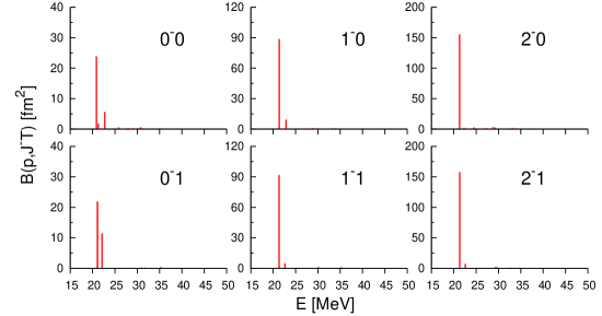
Figure 3: (Color online) The discretized SD reduced transition probabilities of IS and IV0 types from the first excited $0^{+}0$ state of ⁴He as a function of excitation energy. The calculation is done in the Full basis using the AV8^′+3NF interaction. The calculated excitation energy of the $0^{+}0$ state is 20.33 MeV from the ground-state of ⁴He horiuchi12b .

It is interesting to recall the enhanced SD excitations of the first excited state $J^{\pi}T=0_{2}^{+}0$ that is interpreted as having a well developed $3N+N$ (³H+$p$ and ³He+$n$) structure hiyama04 ; horiuchi08 . It is shown in Ref. horiuchi08 that some negative-parity states can also be understood as parity inverted partners of the first excited state and the SD transition strengths from that state are quite enhanced and mostly exhausted by only those negative-parity states. Figure 3 exhibits the SD reduced transition probabilities from the $0_{2}^{+}0$ state as a function of excitation energy. The transition probabilities of both IS and IV0 are very much enhanced, approximately 20-30 times larger than those from the ground state and each of the strengths is concentrated at the respective peak. The excitation energies of the peaks are 20.85, 21.37, 21.30 MeV for $J^{\pi}T=0^{-}0,1^{-}0,2^{-}0$ and 21.10, 21.32, 21.33 MeV for $J^{\pi}T=0^{-}1,1^{-}1,2^{-}1$, respectively. The energy required for the $0_{2}^{+}0$ state to reach the peak position is only $0.5-1.0$ MeV. The neutrino reaction rate would be greatly enhanced if there were such a situation in which a plenty of the first excited states of ⁴He existed in the core collapse star. The situation may, however, be unlikely as the life time of that state is short and its excitation energy (20.21 MeV) is considerably high compared to the typical temperature of the collapsing star woosely90 .

III.2 Spin-dipole strength functions

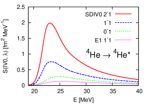
Figure 4: (Color online) Isovector SD strength functions of IV0 type and $E1$ strength function for ⁴He as a function of excitation energy.

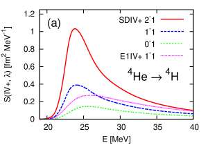
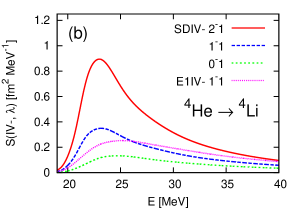
Figure 5: (Color online) Isovector charge-exchange SD strength functions of types IV$+$ (a) and IV$-$ (b) for ⁴He as a function of excitation energy. The excitation energy is counted from the ground state of ⁴He.

In what follows we will present results obtained in the Full basis calculation with the AV8^′+3NF potential using the scaling angle $\theta=17^{\circ}$ unless otherwise mentioned. We count the excitation energy of the continuum state from the calculated ground-state energy of ⁴He that is listed in Table 1 of Ref. horiuchi12b . Preliminary results on the GT and SD strength functions were reported in Refs. horiuchi12b ; horiuchiNIC .

Figure 4 plots the SD strength functions of IV0 type. For the sake of comparison, the $E1$ strength function is also plotted by choosing the $E1$ operator as ${\cal M}_{1\mu}=\sum_{i=1}^{N}{\bm{\rho}_{i}}_{\mu}\frac{1}{2}(1-\tau_{z}(i))$. As seen in the figure, the three SD strength functions show narrower widths at their peaks than the $E1$ strength function. Moreover their peak positions including the $E1$ case well correspond to the observed excitation energies of the four $T=1$ negative-parity states of ⁴He tilley92 . We will discuss this point in Sec. III.3.

Figure 5 displays the charge-exchange SD strength functions of IV$\pm$ type as well as the charge-exchange $E1$ strength that is excited by the operator

$$\mathcal{M}_{1\mu}^{{\rm IV}\pm}=\sum_{i=1}^{N}{\bm{\rho}_{i}}_{\mu}T^{{\rm IV}\pm}_{i}.$$ (22)

Since the mass difference between protons and neutrons is ignored in the present calculation, we need to shift the calculated energies of ⁴H or ⁴Li by $\pm(m_{n}-m_{p})$. This adjustment makes it possible to correctly reproduce the thresholds of ³H+$n$ for ⁴H and ³He+$p$ for ⁴Li, respectively. Similarly to the IV0 case, the excitation energies of the charge-exchange SD peaks correspond to the observed levels of ⁴H and ⁴Li, and their widths are narrow compared to the charge-exchange $E1$ strength function.

We display in Fig. 6 the IS SD strength functions that reflect the $J^{\pi}T=\lambda^{-}0$ continuum states of ⁴He. These IS SD strength functions, especially for the $0^{-}$ and $2^{-}$ cases, show much narrower distribution than the IV strength functions. These peak energies again appear to correspond to the observed $T=0$ negative-parity levels in ⁴He. A close comparison between Figs. 6 and 4 indicates that the $0^{-}$ case is noteworthy compared to the $1^{-}$ and $2^{-}$ cases in that the energy difference in the peak positions of the same $J^{-}$ becomes much larger. As discussed in detail in Refs. horiuchi08 ; horiuchi12b , the reason for this is understood by analyzing the role played by the tensor force among others. In the previous subsection, we mention the three negative-parity states with $T=0$ that are observed slightly above the four-nucleon threshold and are expected to have $d+d$ structure. Though no concentrated strength suggesting such states is seen in Fig. 6, the falloff of the IS SD strength around $28-30$ MeV looks flatter than that of the IV0 case especially in the $J^{\pi}=1^{-}$ state. This indicates that some IS SD strength may exist in that energy region. To be more conclusive, however, a study including $d+d$ configurations explicitly is desirable.

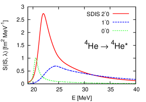
Figure 6: (Color online) The same as Fig. 4 but for the isoscalar SD strength functions.

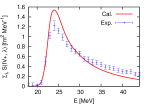
Figure 7: (Color online) Summed isovector SD strength functions for the process from the ground state of ⁴He to ⁴H as a function of excitation energy. Relevant experimental data taken from Ref. nakayama07 are plotted for reference. See text for the details.

To the best of our knowledge, there are no data that can directly be compared to the theoretical strength functions presented above. An only exception is the measurement of the charge-exchange reaction ⁴He(⁷Li,⁷Be$\gamma$) nakayama07 ; nakayama08 , from which the spin-nonflip ($\Delta S=0$) and spin-flip ($\Delta S=1$) components are separated by measuring the 0.43 MeV $\gamma$ ray of ⁷Be in coincidence with the scattered ⁷Be. The former cross section is ascribed to the $E1$ transition, while the latter to the SD transition. The shape of the deduced photoabsorption cross section fairly well agrees with other direct measurements using photons (see Fig. 9 of Ref. horiuchi12a ), but the absolute magnitude is not determined definitively. The SD spectra corresponding to the excitation of the ⁴H continuum from the ground state of ⁴He is extracted from the spin-flip cross section in a similar way. Figure 7 compares the SD strength functions of type IV$+$ with the ‘experiment’. In this figure the theoretical curve represents just a sum of the strength functions with $\lambda=0,1,2$, and the experimental distribution is normalized in such a way that both strength functions give the same strength when integrated in the energy region from $E$=18 to 44 MeV where the experimental data are available. The comparison between theory and experiment in Fig. 7 should thus be taken qualitative as several assumptions are made in the analysis of the experiment. The peak observed at 24 MeV agrees with the calculated one (see also Fig. 5(a)) and certainly it corresponds to the $J^{\pi}T=2^{-}1$ resonance of ⁴H. We see some difference in the shape of the strength function. Two conceivable reasons for it include firstly that the spin-nonflip process can in fact contribute to the SD transition as the ground state of ⁴He contains $S=2$ components and secondly that some higher multipole effects may contribute to the cross section particularly at high energy wakasa11 . The first reason is easily understood if we consider the transition from $(L=S=2)$ to $(L=1,2,3,S=2)$. Further experimental information is needed to make a direct comparison with the calculation.

III.3 Resonance parameters

Table 1: Resonance energies $E_{R}$ and widths $\Gamma$, given in MeV, of negative-parity levels of $A$=4 nuclei. Calculated values are extracted from the complex eigenvalues $E(\theta)$, and the SD and $E1$ strength functions $S(E)$. Experimental data are taken from Ref. tilley92 .

		4H								4He								4Li
		$E_{R}$				$\Gamma$				$E_{R}$				$\Gamma$				$E_{R}$				$\Gamma$
$J^{\pi}T$		$E(\theta)$	$S(E)$	Exp.		$E(\theta)$	$S(E)$	Exp.		$E(\theta)$	$S(E)$	Exp.		$E(\theta)$	$S(E)$	Exp.		$E(\theta)$	$S(E)$	Exp.		$E(\theta)$	$S(E)$	Exp.
$0^{-}0$		–	–	–		–	–	–		20.42	20.54	21.01		0.96	1.06	0.84		–	–	–		–	–	–
$2^{-}0$		–	–	–		–	–	–		21.67	22.03	21.84		2.12	3.10	2.01		–	–	–		–	–	–
$2^{-}1$		24.45	23.82	24.30		5.00	5.29	5.42		23.63	23.11	23.33		4.99	5.58	5.01		23.08	22.99	23.36		5.02	6.53	6.03
$1_{1}^{-}1$		24.68	24.04	24.61		5.32	6.82	6.73		23.86	23.34	23.64		5.31	7.17	6.20		23.28	23.18	23.68		5.36	8.06	7.35
$1^{-}0$		–	–	–		–	–	–		24.32	24.44	24.25		5.40	9.57	6.10		–	–	–		–	–	–
$0^{-}1$		26.51	25.46	26.38		7.60	9.72	8.92		25.67	24.71	25.28		7.60	9.98	7.97		25.12	24.67	25.44		7.69	11.03	9.35
$1_{2}^{-}1$			25.93	27.13			12.80	12.99			25.36	25.95			13.24	12.66			25.15	26.21			13.92	13.51

As noted in Sec. III.2, all the SD and $E1$ strength functions exhibit some common feature: They all have one peak, though the width of the strength distribution depends on the multipolarity $\lambda$ and the isospin $T$. It looks quite reasonable to identify the peak as a resonance. The resonance energy may be identified with the energy where the peak is located. We also estimate the decay width of the resonance by the difference of two excitation energies at which the strength becomes half of the maximum strength at the peak, which agrees with a correct width if the strength function shows the Lorentz distribution. Actually the distribution is not Lorentzian in general as we see below, but this crude estimate should be useful as a guide. Table 1 lists the resonance energies and widths of the negative-parity states of ⁴He, ⁴H, and ⁴Li that are determined in this way. The agreement between theory and experiment is very satisfactory. The average deviation of the calculated resonance energies from experiment is less than 0.4 MeV for ⁴He despite the fact that most of their widths are larger than 5 MeV. The estimated width is also in reasonable agreement with experiment.

A four-nucleon scattering calculation that couples ³H$+p$, ³He$+n$, and $d+d$ channels as well as many pseudo states is performed in Ref. aoyama12 using the same Hamiltonian as the present study. Though the calculated phase shifts for the $J^{\pi}T=0^{-}0$ state show a clear resonance pattern at the energy consistent with the $0^{-}0$ level of ⁴He, the phase shifts of the $2^{-}0$ and $1^{-}0$ states do not rise high enough to enable one to extract the resonance parameter. A more sophisticated analysis is needed to reveal resonances using, for example, the time-delay matrix smith60 ; igarashi04 . In this context we may say that extracting the resonance parameter from the strength function is robust and can be applied to any case where even no sharp resonance is expected.

Since the resonance parameter obtained above is not directly determined from the complex eigenvalue $E_{\nu}(\theta)$ of the Hamiltonian, one may argue that the agreement is fortuitous. Of course it would be very hard to predict the resonance parameter correctly if a chosen operator is such that has only tiny strength to that resonance. It is therefore interesting and important to examine the complex eigenvalues that constitute the basis of the strength function. To this end we rewrite the strength function (12) as

$$S(p,\lambda,E)=\frac{1}{\pi}\sum_{\nu}\frac{\frac{1}{2}\gamma_{\nu}(\theta)\alpha_{\nu}^{p\lambda}(\theta)-(E-\varepsilon_{\nu}(\theta))\beta_{\nu}^{p\lambda}(\theta)}{(E-\varepsilon_{\nu}(\theta))^{2}+\frac{1}{4}(\gamma_{\nu}(\theta))^{2}},$$ (23)

where $\varepsilon_{\nu}(\theta)$, $\gamma_{\nu}(\theta)$, $\alpha_{\nu}(\theta)$, and $\beta_{\nu}(\theta)$ are defined by

$$E_{\nu}(\theta)=\varepsilon_{\nu}(\theta)+E_{0}-\frac{i}{2}\gamma_{\nu}(\theta),$$

$$\sum_{\mu}\tilde{\mathcal{D}}^{p,\nu}_{\lambda\mu}(\theta)\mathcal{D}^{p,\nu}_{\lambda\mu}(\theta)=\alpha_{\nu}^{p\lambda}(\theta)+i\beta_{\nu}^{p\lambda}(\theta).$$ (24)

The first term of the numerator of Eq. (23) gives the Lorentz distribution, while the second term contributes to the background distribution. In principle a resonance may be identified as such $E_{\nu}(\theta)$ that is stationary with respect to the variation of $\theta$ moiseyev98 . Then the strength function (23) has a $\theta$-independent peak around such a stationary energy $\varepsilon_{\nu}$. Resonance parameters of electron and positron complexes are in fact determined very well by examining the $\theta$-trajectory of $E_{\nu}(\theta)$ usukura02 ; suzuki04 . This is possible because $H(\theta)$ for the atomic case has simple structure, $H(\theta)=Te^{-2i\theta}+Ve^{-i\theta}$, where $T$ and $V$ are the kinetic energy and the Coulomb potential energy. In the nuclear case, however, $H(\theta)$ is by far complicated and a large-angle rotation of the nuclear potential may lead to a very long-ranged potential, which, together with inherent difficulties in solutions with the nuclear Hamiltonian, makes an accurate solution of Eq. (11) extremely hard. Therefore, we first look for such eigenvalues that deviate from the rotating-continuum line as possible candidates for a resonance and choose the one that is closest to the peak energy of the strength function.

For the $J^{\pi}T=0^{-}0$ and $2^{-}0$ states, which have a relatively small decay width, we find only one candidate that may correspond to the observed resonance but other $J^{\pi}T$ states have two or three candidates below $4N$ threshold. However, no candidate is found for the $1_{2}^{-}1$ state that is excited by the $E1$ operator. The resonance energies and widths determined in this way are also listed in Table 1. The resonance energy obtained from the complex energy eigenvalue is in excellent agreement with experiment, even better than that determined by the strength function. The width is also satisfactorily reproduced. Two approaches to determining the resonance parameters produce successful results, and they are powerful, robust, and complementary.

Figure 8: Negative-parity levels of $A$=4 nuclei. Excitation energies are referred to the ground-state of ⁴He. Solid, dashed and dotted lines of calculation are based on the complex eigenvalues, the SD and $E1$ strength functions, and bound-state approximation horiuchi12b , respectively. Experimental data are taken from Ref. tilley92 . Levels belonging to the same $J^{\pi}T$ are connected by thin dotted lines.

Figure 8 compares with experiment the resonance energies of the negative-parity states of ⁴He, ⁴H, and ⁴Li that are determined from the complex energy eigenvalues and the strength functions. It is striking that the theory reproduces the experimental spectrum in correct order and moreover closely to the observed excitation energy. The dotted line in the figure denotes the energy obtained with a kind of the real stabilization method hazi70 , that is by diagonalizing the Hamiltonian in the CG-GV basis functions horiuchi12b . Here the SVM search is performed to optimize the parameters of the basis functions by confining the four nucleons in some configuration space. It should be noted, however, that such calculation faces difficulty when dealing with a resonance with a very broad width such as the $1_{2}^{-}$ level of ⁴He, and therefore the resonance energy obtained in that calculation should be taken only approximate.

III.4 Spin-dipole sum rules

Sum rules are related to the energy moment of the strength functions in different order and can be expressed with the ground-state expectation values of appropriate operators from which we can obtain interesting information on the electroweak properties of nuclei  tsuzuki84 ; lipparini89 .

Throughout Sec. III.4 and Appendices A and C we denote the numbers of nucleons, neutrons, and protons by $A$, $N$, and $Z$, respectively. Accordingly the center-of-mass coordinate is $\bm{x}_{A}$ instead of $\bm{x}_{N}$. In the other sections $N$ is used to denote the number of nucleons because the symbol $A$ is reserved to stand for the matrix that appears in Eq. (18).

III.4.1 Non energy-weighted sum rule

Here we discuss the NEWSR for the SD operator

$$m_{0}(p,\lambda)=\int_{0}^{\infty}S(p,\lambda,E)dE.$$ (25)

The use of the closure relation enables us to express the NEWSR to the expectation value of the operator $\sum_{\mu}\mathcal{O}_{\lambda\mu}^{p{\dagger}}\mathcal{O}_{\lambda\mu}^{p}$ with respect to the ground state $\Psi_{0}$. It is convenient to express that operator as a scalar product of the space-space and spin-spin tensors

$$\mathcal{Q}^{p}_{(\kappa)0}=\sum_{i,j=1}^{A}\big{(}[\bm{\rho}_{i}\times\bm{\rho}_{j}]_{\kappa}\cdot[\bm{\sigma}_{i}\times\bm{\sigma}_{j}]_{\kappa}\big{)}{T^{p}_{i}}^{\dagger}T^{p}_{j},$$ (26)

where the rank $\kappa$ can be 0, 1, and 2, and the symbol $(T_{\kappa}\cdot V_{\kappa})=(-1)^{\kappa}\sqrt{2\kappa+1}[T_{\kappa}\times V_{\kappa}]_{00}$ denotes a scalar product of spherical tensors, $T_{\kappa}$ and $V_{\kappa}$. As shown in Eq. (40) of Appendix A, the NEWSR (25) is equivalently expressed, with use of $U_{\lambda\kappa}$ of Eqs. (42) and (43), as

$$m_{0}(p,\lambda)=\sum_{\kappa=0}^{2}U_{\lambda\kappa}\langle\mathcal{Q}^{p}_{(\kappa)0}\rangle.$$ (27)

The expectation value, $\langle\mathcal{Q}^{p}_{(\kappa)0}\rangle=\langle\Psi_{0}|\mathcal{Q}^{p}_{(\kappa)0}|\Psi_{0}\rangle$, can be evaluated using the basis functions (16), (17), and (18), as explained in Appendix B.

In order to check the extent to which the NEWSR is satisfied, we compare $m_{0}(p,\lambda)$ that is calculated separately with Eq. (25) or with Eq. (27). Table 2 lists the calculated NEWSR for the SD strength functions. We also list the values of $\langle\mathcal{Q}^{p}_{(\kappa)0}\rangle$ in Table 3 for the sake of discussions below. As seen in Table 2, the two different ways of calculating the sum rules give virtually the same result for both cases of AV8^′+3NF and G3RS+3NF interactions, which is never trivial because we use the fully correlated ground-state wave function for ⁴He. The perfect agreement confirms that the basis functions prepared for the description of the SD excitation are sufficient enough to account for all the strength in the continuum. The NEWSR calculated with Eq. (27) for the Minnesota (MN) potential MN is also listed in Table 2. A comparison of the central MN force case with the realistic potentials will be useful to know how much the sum rule is affected by the tensor force.

Table 2: Non energy-weighted sum rules of the SD strength functions, in units of fm², calculated from different models for the nucleon-nucleon potentials. The sum rules calculated by Eqs. (25) and (27) are labeled $m_{0}(p,\lambda)$ and SR, respectively.

		AV8′+3NF									G3RS+3NF									MN
		IS			IV0			IV$\pm$			IS			IV0			IV$\pm$			IS		IV0		IV$\pm$
$\lambda$		$m_{0}(p,\lambda)$	SR		$m_{0}(p,\lambda)$	SR		$m_{0}(p,\lambda)$	SR		$m_{0}(p,\lambda)$	SR		$m_{0}(p,\lambda)$	SR		$m_{0}(p,\lambda)$	SR		SR		SR		SR
0		2.71	2.71		4.59	4.59		2.30	2.30		2.83	2.84		4.74	4.74		2.37	2.37		3.90		3.49		1.74
1		12.16	12.17		9.35	9.36		4.68	4.68		12.64	12.65		9.72	9.73		4.86	4.86		11.71		10.46		5.23
2		17.98	18.02		18.36	18.38		9.18	9.19		18.77	18.79		19.02	19.04		9.51	9.52		19.51		17.43		8.71

Table 3: Expectation values of $\mathcal{Q}_{(\kappa)0}^{p}$ and its one- and two-body terms with respect to the ground state of ⁴He. Values are given in units of fm².

		AV8′+3NF				G3RS+3NF				MN
		IS	IV0	IV$\pm$		IS	IV0	IV$\pm$		IS	IV0	IV$\pm$
$\langle\mathcal{Q}_{(0)0}^{p}\rangle$		10.97	10.78	5.39		11.42	11.17	5.59		11.71	10.46	5.23
$\langle\mathcal{Q}_{(0)0}^{p(1)}\rangle$		8.41	8.41	4.21		8.66	8.66	4.33		7.96	7.96	3.98
$\langle\mathcal{Q}_{(0)0}^{p(2)}\rangle$		2.56	2.37	1.18		2.76	2.51	1.25		3.75	2.50	1.25
$\langle\mathcal{Q}_{(1)0}^{p}\rangle$		0.21	$-$0.08	$-$0.04		0.24	$-$0.09	$-$0.04		0.00	0.00	0.00
$\langle\mathcal{Q}_{(1)0}^{p(1)}\rangle$		–	–	–		–	–	–		–	–	–
$\langle\mathcal{Q}_{(1)0}^{p(2)}\rangle$		0.21	$-$0.08	$-$0.04		0.24	$-$0.09	$-$0.04		0.00	0.00	0.00
$\langle\mathcal{Q}_{(2)0}^{p}\rangle$		$-$2.61	2.92	1.46		$-$2.68	2.97	1.49		0.00	0.00	0.00
$\langle\mathcal{Q}_{(2)0}^{p(1)}\rangle$		–	–	–		–	–	–		–	–	–
$\langle\mathcal{Q}_{(2)0}^{p(2)}\rangle$		$-$2.61	2.92	1.46		$-$2.68	2.97	1.49		0.00	0.00	0.00

Among the three expectation values of $\langle\mathcal{Q}^{p}_{(\kappa)0}\rangle$ in Eq. (27), the $\kappa=0$ term gives a dominant contribution to the NEWSR. See Table 3. This is obviously because the major component of the ground state of ⁴He is $S=0$ and it has a non-vanishing expectation value only for $\mathcal{Q}^{p}_{(0)0}$. In this limiting case $m_{0}(p,\lambda)$ is proportional to $U_{\lambda 0}$. Therefore the $\lambda$-dependence of the NEWSR turns out to be $1:3:5$ for $\lambda=0,\,1,\,2$, independently of $p$. This rule is confirmed in the MN case of Table 2. The deviation from this ratio is due to the contributions of other $\mathcal{Q}^{p}_{(\kappa)0}$ terms, especially the $\kappa=2$ term. The $\mathcal{Q}^{p}_{(2)0}$ term contributes to the NEWSR through the coupling matrix element between the $S=0$ and $S=2$ components of the ground state of ⁴He. Since the admixture of the $S=2$ component is primarily determined by the tensor force, the deviation reflects the tensor correlations in the ground state. Neglecting the minor contribution of $\mathcal{Q}^{p}_{(1)0}$, Eq. (27) suggests that $m_{0}(p,\lambda)$ is very well approximated by

$$m_{0}(p,0) =\frac{1}{3}(\langle\mathcal{Q}^{p}_{(0)0}\rangle-\langle\mathcal{Q}^{p}_{(1)0}\rangle+\langle\mathcal{Q}^{p}_{(2)0}\rangle),$$

$$m_{0}(p,1) =m_{0}(p,0)+\frac{1}{2}(\langle\mathcal{Q}^{p}_{(1)0}\rangle-3\langle\mathcal{Q}^{p}_{(2)0}\rangle)$$

$$\approx m_{0}(p,0)-\frac{3}{2}\langle\mathcal{Q}^{p}_{(2)0}\rangle,$$

$$m_{0}(p,2) =\frac{5}{3}m_{0}(p,0)+\frac{1}{2}(5\langle\mathcal{Q}^{p}_{(1)0}\rangle-3\langle\mathcal{Q}^{p}_{(2)0}\rangle)$$

$$\approx\frac{5}{3}m_{0}(p,0)-\frac{3}{2}\langle\mathcal{Q}^{p}_{(2)0}\rangle.$$ (28)

Thus the deviation of the ratio from $1:3:5$ is simply controlled by $-\frac{3}{2}\langle\mathcal{Q}^{p}_{(2)0}\rangle$, which is very well satisfied in the examples of Table 2. Since $\langle\mathcal{Q}^{p}_{(2)0}\rangle$ is negative for $p={\rm IS}$, the ratio further increases from $1:3:5$, whereas it is positive for $p={\rm IV0}$ and IV$\pm$, and the ratio approximately reduces to $1:2:4$.

As discussed above, $\langle\mathcal{Q}^{p}_{(\kappa)0}\rangle$ plays a central role to determine the NEWSR for the SD strength functions. Inverting Eq. (27) makes it possible to express $\langle\mathcal{Q}^{p}_{(\kappa)0}\rangle$ as a sum, over the multipole $\lambda$, of the NEWSR

$$\langle\mathcal{Q}^{p}_{(\kappa)0}\rangle=\sum_{\lambda=0}^{2}U^{-1}_{\ \ \kappa\lambda}m_{0}(p,\lambda),$$ (29)

where $U^{-1}$ is the inverse matrix of $U$ as given in Eq. (44). If the NEWSR for all $\lambda$ are experimentally measured, the above equation indicates that $\langle\mathcal{Q}^{p}_{(\kappa)0}\rangle$ for all $\kappa$ can be determined from experiment. Some examples are

$$3\langle\mathcal{Q}^{p}_{(0)0}\rangle=m_{0}(p,0)+m_{0}(p,1)+m_{0}(p,2),$$

$$6\langle\mathcal{Q}^{p}_{(2)0}\rangle=10m_{0}(p,0)-5m_{0}(p,1)+m_{0}(p,2).$$ (30)

To clarify the physical meaning of the operator $\mathcal{Q}^{p}_{(\kappa)0}$, it is instructive to decompose it into one- and two-body terms:

$$\mathcal{Q}^{p}_{(\kappa)0}=\mathcal{Q}^{p(1)}_{(\kappa)0}+\mathcal{Q}^{p(2)}_{(\kappa)0},$$ (31)

where

$$\mathcal{Q}^{p(1)}_{(\kappa)0}=\delta_{\kappa 0}\sum_{i=1}^{A}\bm{\rho}_{i}^{2}{T^{p}_{i}}^{\dagger}T^{p}_{i},$$

$$\mathcal{Q}^{p(2)}_{(\kappa)0}=\sum_{j>i=1}^{A}\big{(}[\bm{\rho}_{i}\times\bm{\rho}_{j}]_{\kappa}\cdot[\bm{\sigma}_{i}\times\bm{\sigma}_{j}]_{\kappa}\big{)}T^{p}_{ij}$$ (32)

with

$$T^{p}_{ij}={T^{p}_{i}}^{\dagger}T^{p}_{j}+{T^{p}_{j}}^{\dagger}T^{p}_{i}.$$ (33)

The isospin operators in Eq. (32) are simplified with use of Eq. (A2): ${T^{p}_{i}}^{\dagger}T^{p}_{i}$ is 1 for $p={\rm IS}$, IV0, and $(1\mp\tau_{z}(i))/2$ for $p={\rm IV}\pm$, whereas $T^{p}_{ij}$ is 2 for $p={\rm IS}$, $2\tau_{z}(i)\tau_{z}(j)$ for $p={\rm IV0}$, and $((\bm{\tau}(i)\cdot\bm{\tau}(j))-\tau_{z}(i)\tau_{z}(j))/2$ for $p={\rm IV}\pm$, respectively. The one-body term is spin-independent and appears only for $\kappa=0$, which gives the largest contribution to the NEWSR. The two-body term with $\kappa=2$ is particularly interesting because it contains the tensor operator characteristic of the one-pion-exchange potential. See Appendix A for detail.

The expectation value of the one-body term is expressed in terms of the root-mean-square radius of nucleon distribution in the ground state

$$\langle\mathcal{Q}^{{\rm IS}(1)}_{(0)0}\rangle=\langle\mathcal{Q}^{{\rm IV0}(1)}_{(0)0}\rangle=A\langle r_{N}^{2}\rangle,$$

$$\langle\mathcal{Q}^{{\rm IV+}(1)}_{(0)0}\rangle=Z\langle r_{p}^{2}\rangle,\quad\langle\mathcal{Q}^{{\rm IV-}(1)}_{(0)0}\rangle=N\langle r_{n}^{2}\rangle.$$ (34)

Noting that the two-body term $\mathcal{Q}^{{\rm IV}+(2)}_{(\kappa)0}$ is identical to $\mathcal{Q}^{{\rm IV}-(2)}_{(\kappa)0}$ for any $\kappa$, we obtain the following well-known relation between the NEWSR gaarde81

$$m_{0}({\rm IV}-,\lambda)-m_{0}({\rm IV}+,\lambda)=\frac{2\lambda+1}{3}\big{(}N\langle r_{n}^{2}\rangle-Z\langle r_{p}^{2}\rangle\big{)}.$$ (35)

This difference vanishes in the present case because the isospin impurity of the ground-state of ⁴He is ignored.

III.4.2 Energy-weighted sum rule

Now we discuss the EWSR for the SD operator. The SD EWSR can be derived in the same manner as the $E1$ operator, and it is expressed as

$$m_{1}(p,\lambda) =\int_{0}^{\infty}ES(p,\lambda,E)dE$$

$$=\langle X^{p}_{(\lambda)0}(H)\rangle,$$ (36)

where $X^{p}_{(\lambda)0}(H)$ denotes the double commutator of the Hamiltonian with the SD operator

$$X^{p}_{(\lambda)0}(H)=\frac{1}{2}\sum_{\mu}[\mathcal{O}_{\lambda\mu}^{p\dagger},[H,\mathcal{O}_{\lambda\mu}^{p}]].$$ (37)

The double commutator of the kinetic energy operator $T=\sum_{i=1}^{A}T_{i}-T_{\rm cm}$ is worked out in Appendix C. The commutator was considered in Ref. tsuzuki79 for IS and IV0 cases. The result for all SD cases is summarized as

$$X^{p}_{(\lambda)0}(T)=\frac{(A-1)\hbar^{2}}{2Am_{N}}(2\lambda+1)N^{p}$$

$$-\frac{\hbar^{2}}{6Am_{N}}(2\lambda+1)\sum_{j>i=1}^{A}(\bm{\sigma}_{i}\cdot\bm{\sigma}_{j})T^{p}_{ij}$$

$$-\frac{i\hbar}{6m_{N}}(2\lambda+1)\sum_{i=1}^{A}\big{(}\bm{\rho}_{i}\cdot(\bm{p}_{i}-\textstyle{\frac{1}{A}}\bm{P}_{\rm tot})\big{)}[{T^{p}_{i}}^{\dagger},T^{p}_{i}]$$

$$+\frac{\hbar}{6m_{N}}C_{\lambda}^{p}\sum_{i=1}^{A}\big{(}(\bm{\rho}_{i}\times(\bm{p}_{i}-\textstyle{\frac{1}{A}}\bm{P}_{\rm tot}))\cdot\bm{\sigma}_{i}\big{)},$$ (38)

where $\bm{P}_{\rm tot}=\sum_{i=1}^{A}{\bm{p}}_{i}$ is the total momentum and $C^{p}_{\lambda}$ is related to $C_{\lambda}$ of Eq. (C7) as

$$C_{\lambda}^{\rm IS}=C_{\lambda}^{\rm IV0}=C_{\lambda},\quad C_{\lambda}^{{\rm IV}+}=C_{\lambda}^{{\rm IV}-}=\frac{1}{2}C_{\lambda},$$ (39)

and $N^{p}=\sum_{i=1}^{A}T_{i}^{p}{T^{p}_{i}}^{\dagger}$ reduces to $A$ for $p={\rm IS}$, IV0, $A-Z$ for $p={\rm IV}+$, and $A-N$ for $p={\rm IV}-$, respectively. The isospin commutator $[{T^{p}_{i}}^{\dagger},T^{p}_{i}]$ vanishes for $p={\rm IS}$ and IV0, while it reduces to $\mp\tau_{z}(i)$ for $p={\rm IV}\pm$. The round bracket $(\bm{a}\times\bm{b})$ stands for the vector product of $\bm{a}$ and $\bm{b}$, $(\bm{a}\times\bm{b})_{\mu}=-\sqrt{2}i[\bm{a}\times\bm{b}]_{1\mu}$.

We name the four terms on the right-hand side of Eq. (38) as model-independent (MI), spin-spin (SS), dilation (DL), and spin-orbit (SO) terms, respectively. The name of dilation is adopted because $\big{(}\bm{\rho}_{i}\cdot(\bm{p}_{i}-\textstyle{\frac{1}{A}}\bm{P}_{\rm tot})\big{)}$ is a generator for the dilation operator. The MI term makes a contribution to the SD EWSR, independently of the ground-state wave function. Thus the kinetic energy contribution to the EWSR becomes model-independent in so far as the contribution of the other terms can be neglected compared to the MI term. For a fixed $p$ the $\lambda$-dependence of each term is simply given by $2\lambda+1$ except for the SO term, which changes according to the ratio of $2:3:(-5)$ for $\lambda=0,1,2$. On the other hand, for a fixed $\lambda$ the $p$-dependence of the four terms is a little complicated. The MI term changes in proportion to $A:A:A-Z:A-N$, while the SO term is in ratio of $1:1:1/2:1/2$ for $p={\rm IS}$, IV0, IV$+$, IV$-$, respectively. The DL term identically vanishes for $p={\rm IS}$ and IV0, and furthermore it turns out to have no contribution to the EWSR even for $p={\rm IV}\pm$ because no isospin mixing is taken into account in our ground state of ⁴He.

Table 4 lists the values of $m_{1}(p,\lambda)$ together with the contributions of the kinetic energy term and its four terms to the EWSR calculated using the AV8^′+3NF and G3RS+3NF potentials. The EWSR slightly depends on the potential models particularly for the IS SD strengths. Even in those cases the contribution of the kinetic energy to the EWSR remains almost the same. The contribution of the MI term to $\langle X_{(\lambda)0}^{p}(T)\rangle$ is found to be more than 74 % for all the cases, and really occupies a main portion of the kinetic energy contribution. The two interactions give almost the same contribution for the SS terms. Though the SO terms show some dependence on the interactions, the kinetic energy contributions $\langle X^{p}_{(\lambda)0}(T)\rangle$ are found to be approximately model-independent.

Table 4: Energy-weighted sum rules of the SD strength functions, $m_{1}(p,\lambda)$, in units of fm²MeV, calculated from different models for the nucleon-nucleon potentials. Contribution of each term of the kinetic energy to the sum rule is also listed. See text for the details.

		AV8′+3NF
		IS				IV0				IV$+$				IV$-$
		$\lambda=0$	$\lambda=1$	$\lambda=2$		$\lambda=0$	$\lambda=1$	$\lambda=2$		$\lambda=0$	$\lambda=1$	$\lambda=2$		$\lambda=0$	$\lambda=1$	$\lambda=2$
$m_{1}(p,\lambda)$		126	782	949		218	450	766		110	227	389		109	225	383
$\langle X_{(\lambda)0}^{p}(T)\rangle$		74.4	227	392		78.2	239	411		39.1	119	205		39.1	119	205
MI		62.2	187	311		62.2	187	311		31.1	93.3	156		31.1	93.3	156
SS		14.9	44.6	74.3		18.7	55.9	93.2		9.32	27.9	46.6		9.32	27.9	46.6
DL		–	–	–		–	–	–		0.00	0.00	0.00		0.00	0.00	0.00
SO		$-$2.62	$-$3.92	6.54		$-$2.62	$-$3.92	6.54		$-$1.31	$-$1.96	3.27		$-$1.31	$-$1.96	3.27
$m_{1}(p,\lambda)-\langle X_{(\lambda)0}^{p}(T)\rangle$		51.5	555	557		139	211	355		71.3	108	183		70.1	106	178
		G3RS+3NF
		IS				IV0				IV$+$				IV$-$
		$\lambda=0$	$\lambda=1$	$\lambda=2$		$\lambda=0$	$\lambda=1$	$\lambda=2$		$\lambda=0$	$\lambda=1$	$\lambda=2$		$\lambda=0$	$\lambda=1$	$\lambda=2$
$m_{1}(p,\lambda)$		111	697	843		202	426	723		104	216	370		102	213	363
$\langle X_{(\lambda)0}^{p}(T)\rangle$		73.2	227	403		76.3	236	419		38.1	118	209		38.1	118	209
MI		62.2	187	311		62.2	187	311		31.1	93.3	156		31.1	93.3	156
SS		16.0	47.9	79.8		19.0	57.1	95.1		9.51	28.5	47.6		9.51	28.5	47.6
DL		–	–	–		–	–	–		0.00	0.00	0.00		0.00	0.00	0.00
SO		$-$4.97	$-$7.45	12.4		$-$4.97	$-$7.45	12.4		$-$2.48	$-$3.73	6.21		$-$2.48	$-$3.73	6.21
$m_{1}(p,\lambda)-\langle X_{(\lambda)0}^{p}(T)\rangle$		37.8	470	439		126	189	304		65.5	97.8	160		63.5	94.6	153

The enhancement of the computed sum rule (36) compared to $\langle X_{(\lambda)0}^{p}(T)\rangle$ indicates the contribution of the potential energy to the EWSR. The enhancement factor for the $E1$ operator is $1.0-1.1$ for the present nuclear forces horiuchi12a . The AV8^′ potential has a stronger tensor component than the G3RS potential. Because of this the tensor potential ($S_{ij}\bm{\tau}_{i}\cdot\bm{\tau}_{j}$) of the AV8^′ potential gives the larger contribution to the $E1$ EWSR. In the SD case, however, the enhancement is more complicated and depends on both multipolarity $\lambda$ and isospin label $p$. To elucidate this further, we have to calculate the double commutator for each piece of the nucleon-nucleon potential as in the kinetic energy and evaluate its ground-state expectation value.

IV Conclusions

We study both isovector and isoscalar spin-dipole (SD) strength functions in four-body calculations using realistic nuclear forces. Two different potentials are employed to see the sensitivity on the $D$-state probability produced by the tensor correlation. The SD excitation is built on the ground state of ⁴He that is described accurately with use of explicitly correlated Gaussian bases. The continuum states including two- and three-body decay channels are discretized in the correlated Gaussians with aid of the complex scaling method.

Experimental data that can directly be compared to the calculation are presently only the resonance parameters of the negative-parity levels of $A=4$ nuclei. Both the resonance energies and widths deduced from the SD and electric-dipole strength functions or the eigenvalues of the complex-scaled Hamiltonian are all in fair agreement with experiment. This success is never trivial considering that most of the resonances among 15 levels have broad widths larger than 5 MeV. A combined use of both complex energies and appropriate strength functions provides us with a robust tool to determine resonance parameters.

The non energy-weighted sum rule (NEWSR) of the SD strength function is investigated by relating it to the expectation values of three scalar products of the space-space and spin-spin tensors with respect to the ground state of ⁴He. It turns out that our model space satisfies the NEWSR for each SD operator perfectly. The tensor operator of rank 2, $\mathcal{Q}^{p}_{(2)0}$, is sensitive to the $D$-state correlation in the ground state induced by the tensor force, and it is mainly responsible for distorting the ratio of the NEWSRs for the multipolarity $\lambda=0,1,2$ from the uncorrelated ratio of $1:3:5$. An experimental observation of this ratio is desirable since it may lead us to reveal the degree of tensor correlations in the ground state. The energy-weighted sum rule (EWSR) for the SD operator is also examined. A formula is derived to calculate the contribution of the kinetic energy to the EWSR. The difference between the EWSR and the kinetic energy contribution shows some dependence on $\lambda$ as wells as the isospin character of the SD operator. Further study is needed to clarify the origin of its dependence by analyzing the contribution of each piece of the nuclear potential.

Other $T=0$ resonances with $0^{-},\,1^{-},\,2^{-}$ and $1^{+},\,2^{+}$ exist in ⁴He above and below the $2n+2p$ threshold. It would be interesting to investigate these levels by the isoscalar SD excitation and some appropriate excitations produced by e.g., isoscalar quadrupole, magnetic dipole, and spin-quadrupole operators with further attention being paid to $d+d$ type configurations.

The SD strength functions are important inputs for evaluating neutrino-nucleus reaction rates. A calculation of neutrino-⁴He reaction rate is in progress as a consequence of the present study. It is desirable that the predicted SD strength functions are tested with experimental measurements in order for such reaction rate calculation to be precise.

Appendix A Multipole decomposition of the spin-dipole non energy-weighted sum rule

Here we derive Eqs. (26) and (27) by decomposing the operator $\sum_{\mu}\mathcal{O}_{\lambda\mu}^{p\dagger}\mathcal{O}_{\lambda\mu}^{p}$ into multipoles. Substituting Eq. (1) in $\sum_{\mu}\mathcal{O}_{\lambda\mu}^{p\dagger}\mathcal{O}_{\lambda\mu}^{p}$ and recoupling the coordinate and spin operators, we obtain

$$\sum_{\mu}\mathcal{O}_{\lambda\mu}^{p\dagger}\mathcal{O}_{\lambda\mu}^{p}$$

$$=(-1)^{\lambda}\sum_{i,j=1}^{A}\big{(}[\bm{\rho}_{i}\times\bm{\sigma}_{i}]_{\lambda}\cdot[\bm{\rho}_{j}\times\bm{\sigma}_{j}]_{\lambda}\big{)}{T^{p}_{i}}^{\dagger}T^{p}_{j}$$

$$=\sum_{\kappa}U_{\lambda\kappa}\mathcal{Q}^{p}_{(\kappa)0}.$$ (40)

The isospin operator ${T^{p}_{i}}^{\dagger}T^{p}_{j}$ reads

$$1,\quad\tau_{z}(i)\tau_{z}(j),\quad(\bm{t}_{i}\cdot\bm{t}_{j})-t_{z}(i)t_{z}(j)\pm i(\bm{t}_{i}\times\bm{t}_{j})_{z}$$ (41)

for $p={\rm IS}$, IV0, and IV$\pm$, respectively. The coefficient $U_{\lambda\kappa}$ is expressed by unitary Racah coefficients $U$ as

$$U_{\lambda\kappa}=(-1)^{\lambda}\sqrt{\frac{2\lambda+1}{2\kappa+1}}U(1111,\lambda\kappa),$$ (42)

or more explicitly

$$(U_{\lambda\kappa})=\begin{pmatrix}\frac{1}{3}&-\frac{1}{3}&\frac{1}{3}\\ 1&-\frac{1}{2}&-\frac{1}{2}\\ \frac{5}{3}&\frac{5}{6}&\frac{1}{6}\end{pmatrix},$$ (43)

where both row and column labels, $\lambda$ and $\kappa$, are arranged in order of 0, 1, and 2. The inverse of the matrix $(U_{\lambda\kappa})$,

$$({U^{-1}}_{\kappa\lambda})=\begin{pmatrix}\frac{1}{3}&\frac{1}{3}&\frac{1}{3}\\ -1&-\frac{1}{2}&\frac{1}{2}\\ \frac{5}{3}&-\frac{5}{6}&\frac{1}{6}\\ \end{pmatrix},$$ (44)

is used to obtain the expectation value of $\mathcal{Q}^{p}_{(\kappa)0}$ with respect to the ground state as discussed in Sec. III.4.1. See Eq. (29).

The multipole operator $\mathcal{Q}^{p}_{(\kappa)0}$ consists of one- and two-body terms

$$\mathcal{Q}^{p}_{(\kappa)0}=\mathcal{Q}^{p(1)}_{(\kappa)0}+\mathcal{Q}^{p(2)}_{(\kappa)0}$$ (45)

as shown in Eq. (32). The two-body term with $\kappa=2$ is of particular interest because it contains the tensor operator. To see this, it is convenient to rewrite $\mathcal{Q}^{p(2)}_{(\kappa)0}$ in terms of the relative and center-of-mass coordinates of two nucleons rather than the single-particle like coordinates, $\bm{\rho}_{i}$ and $\bm{\rho}_{j}$. By introducing the coordinates $\bm{r}_{ij}$ and $\bm{R}_{ij}$ by

$$\bm{r}_{ij} =\bm{\rho}_{i}-\bm{\rho}_{j}=\bm{r}_{i}-\bm{r}_{j},$$

$$\bm{R}_{ij} =\frac{1}{2}(\bm{\rho}_{i}+\bm{\rho}_{j})=\frac{1}{2}(\bm{r}_{i}+\bm{r}_{j})-\bm{x}_{A},$$ (46)

$\mathcal{Q}^{p(2)}_{(\kappa)0}$ is decomposed to three terms:

$$\mathcal{Q}^{p(2)}_{(\kappa)0}=\mathcal{Q}^{p(2)r}_{(\kappa)0}+\mathcal{Q}^{p(2)R}_{(\kappa)0}+\delta_{\kappa 1}\mathcal{Q}^{p(2)rR}_{(1)0},$$ (47)

where

$$\mathcal{Q}^{p(2)r}_{(\kappa)0}=-\frac{1}{4}\sum_{j>i=1}^{A}\big{(}[\bm{r}_{ij}\times\bm{r}_{ij}]_{\kappa}\cdot[\bm{\sigma}_{i}\times\bm{\sigma}_{j}]_{\kappa}\big{)}T^{p}_{ij},$$

$$\mathcal{Q}^{p(2)R}_{(\kappa)0}=\sum_{j>i=1}^{A}\big{(}[\bm{R}_{ij}\times\bm{R}_{ij}]_{\kappa}\cdot[\bm{\sigma}_{i}\times\bm{\sigma}_{j}]_{\kappa}\big{)}T^{p}_{ij},$$

$$\mathcal{Q}^{p(2)rR}_{(1)0}=\sum_{j>i=1}^{A}\big{(}[\bm{r}_{ij}\times\bm{R}_{ij}]_{1}\cdot[\bm{\sigma}_{i}\times\bm{\sigma}_{j}]_{1}\big{)}T^{p}_{ij}.$$ (48)

The operators $\mathcal{Q}^{p(2)r}_{(\kappa)0}$ and $\mathcal{Q}^{p(2)R}_{(\kappa)0}$ have non-vanishing contributions only for $\kappa=0$ and 2. It is easy to see that the $\mathcal{Q}^{p(2)r}_{(2)0}$ term contains the tensor operator $S_{ij}$.

Appendix B Calculation of the matrix elements of quadratic spatial tensors

In this appendix, we give a formula of calculating the matrix element of $\mathcal{Q}^{p}_{(\kappa)0}$, Eq. (26). The spin-isospin part can easily be evaluated in our spin and isospin functions, Eq. (17), so that we focus on the matrix element of the spatial part. As is clear from Eqs. (32) and (48), the spatial tensor operators have the form $[\bm{a}\times\bm{b}]_{\kappa\mu}$, where $\bm{a}$ and $\bm{b}$ are vectors that represent one of the various coordinates, $\bm{\rho}_{i},\ \bm{\rho}_{j},\ \bm{r}_{ij},\ \bm{R}_{ij}$. It is useful to note that any of these coordinates can be expressed as a linear combination of the relative coordinate set $\bm{x}$: $\bm{a}=\sum_{i=1}^{N-1}\omega_{i}\bm{x}_{i}=\tilde{\omega}{\bm{x}}$, and $\bm{b}=\sum_{i=1}^{N-1}\zeta_{i}\bm{x}_{i}=\tilde{\zeta}{\bm{x}}$, where $\omega$ and $\zeta$ are both $(N-1)$-dimensional column vectors. Therefore it is sufficient to show how we can evaluate the quadratic spatial tensor operators, $[\tilde{\omega}\bm{x}\times\tilde{\zeta}\bm{x}]_{\kappa\mu}$, with the basis functions (18). A detailed method of evaluation is presented in Ref. suzuki08 , and here we follow its formulation and notation.

First we calculate the matrix element between the generating function

$$g(\bm{s},A,\bm{x})=\exp\Big{(}-\frac{1}{2}\tilde{\bm{x}}A\bm{x}+\tilde{\bm{s}}\bm{x}\Big{)},$$ (49)

where $\bm{s}$ is an $(N-1)$-dimensional column vector whose $i$th element is a 3-dimensional vector $\bm{s}_{i}$, and $\tilde{\bm{s}}\bm{x}$ is a short-hand notation of $\sum_{i=1}^{N-1}\bm{s}_{i}\cdot{\bm{x}}_{i}$. As given in Ref. svm , it reads

$$\left<g(\bm{s}^{\prime},A^{\prime},\bm{x})\right|[\tilde{\omega}\bm{x}\times\tilde{\zeta}\bm{x}]_{\kappa\mu}\left|g(\bm{s},A,\bm{x})\right>$$

$$=\left\{-\sqrt{3}\delta_{\kappa 0}\delta_{\mu 0}{\rm Tr}\left(B^{-1}\omega\tilde{\zeta}\right)+\left[\tilde{\omega}B^{-1}\bm{v}\times\tilde{\zeta}B^{-1}\bm{v}\right]_{\kappa\mu}\right\}\left(\frac{(2\pi)^{N-1}}{{\rm det}B}\right)^{\frac{3}{2}}\text{e}^{\frac{1}{2}\tilde{\bm{v}}B^{-1}\bm{v}},$$ (50)

where Tr stands for a trace and

$$B=A+A^{\prime},\quad\bm{v}=\bm{s}+\bm{s}^{\prime}.$$ (51)

Using the $(N-1)$-dimensional column vector $u_{i}$ specifying the GV we express $\bm{s}$ and $\bm{s}^{\prime}$ as $\bm{s}=\lambda_{1}\bm{e}_{1}u_{1}+\lambda_{2}\bm{e}_{2}u_{2}$ and $\bm{s}^{\prime}=\lambda_{3}\bm{e}_{3}u_{3}+\lambda_{4}\bm{e}_{4}u_{4}$, where a unit vector $\bm{e}_{i}$ ($(\bm{e}_{i}\cdot\bm{e}_{i})=1$) and a parameter $\lambda_{i}$ are introduced to manipulate the calculation of the sought matrix element. See Ref. suzuki08 for details. The second term in the curly bracket and the exponential function of Eq. (50) is simplified to

$$\left[\tilde{\omega}B^{-1}\bm{v}\times\tilde{\zeta}B^{-1}\bm{v}\right]_{\kappa\mu}\to\sum_{i,j}f_{i}g_{j}\lambda_{i}\lambda_{j}[\bm{e}_{i}\times\bm{e}_{j}]_{\kappa\mu},$$

$$\text{e}^{\frac{1}{2}\tilde{\bm{v}}B^{-1}\bm{v}}\to\text{e}^{\sum_{i<j}\rho_{ij}\lambda_{i}\lambda_{j}\bm{e}_{i}\cdot\bm{e}_{j}},$$ (52)

where

$$\rho_{ij}=\tilde{u}_{i}B^{-1}u_{j},\quad f_{i}=\tilde{\omega}B^{-1}u_{i},\quad g_{j}=\tilde{\zeta}B^{-1}u_{j}.$$ (53)

Here the arrow symbol indicates that both sides are equal as long as the calculation of the sought matrix element is concerned. That is, any terms that have $\lambda_{i}^{2}(\bm{e}_{i}\cdot\bm{e}_{i})=\lambda_{i}^{2}$ dependence make no contribution to the matrix element, so that they can be dropped.

(i) $\kappa=0$ case

In this case the term $[\tilde{\omega}B^{-1}\bm{v}\times\tilde{\zeta}B^{-1}\bm{v}]_{00}$ produces the same structure, with respect to $\lambda_{i}\lambda_{j}(\bm{e}_{i}\cdot\bm{e}_{j})$, as the kinetic and mean square distance operators. See Appendix B.2 of Ref. suzuki08 . The matrix element is

$$\left<F_{(L_{3}L_{4})LM}(u_{3},u_{4},A^{\prime},\bm{x})\right|[\tilde{\omega}\bm{x}\times\tilde{\zeta}\bm{x}]_{00}\left|F_{(L_{1}L_{2})LM}(u_{1},u_{2},A,\bm{x})\right>$$

$$=-\frac{1}{\sqrt{3}}\Bigl{\{}3{\rm Tr}(B^{-1}\omega\tilde{\zeta})+\sum_{i<j}(f_{i}g_{j}+f_{j}g_{i})\frac{\partial}{\partial\rho_{ij}}\Bigr{\}}\left<F_{(L_{3}L_{4})LM}(u_{3},u_{4},A^{\prime},\bm{x})|F_{(L_{1}L_{2})LM}(u_{1},u_{2},A,\bm{x})\right>.$$ (54)

Compare this expression with Eq. (B.17) suzuki08 . A formula for the overlap matrix element, $\langle F_{(L_{3}L_{4})LM}(u_{3},u_{4},A^{\prime},\bm{x})|F_{(L_{1}L_{2})LM}(u_{1},u_{2},A,\bm{x})\rangle$, is given in Eq. (B.10) suzuki08 .

(ii) $\kappa=1$ case

The $\kappa=1$ case can be evaluated in exactly the same way as the spin-orbit matrix element of Ref. suzuki08 . The result is

$$\left<F_{(L_{3}L_{4})L^{\prime}M^{\prime}}(u_{3},u_{4},A^{\prime},\bm{x})\right|[\tilde{\omega}\bm{x}\times\tilde{\zeta}\bm{x}]_{1\mu}\left|F_{(L_{1}L_{2})LM}(u_{1},u_{2},A,\bm{x})\right>$$

$$=-\frac{4\pi}{\sqrt{3}}\frac{(-1)^{L_{1}+L_{2}+L+L^{\prime}}}{\sqrt{2L^{\prime}+1}}\left<LM1\mu|L^{\prime}M^{\prime}\right>\sum_{l>k=1}^{4}(f_{k}g_{l}-f_{l}g_{k})(-1)^{\bar{L}_{1}+\bar{L}_{2}}\left(\prod_{i=1}^{4}\frac{B_{L_{i}}}{B_{\bar{L}_{i}}}\right)$$

$$\times\sum_{\bar{L}}\sqrt{2\bar{L}+1}Z_{2}(1\bar{L}_{1}\bar{L}_{2}\bar{L}_{3}\bar{L}_{4}\bar{L},LL^{\prime};kl)\left<F_{(\bar{L}_{3}\bar{L}_{4})\bar{L}\bar{M}}(u_{3},u_{4},A^{\prime},\bm{x})|F_{(\bar{L}_{1}\bar{L}_{2})\bar{L}\bar{M}}(u_{1},u_{2},A,\bm{x})\right>.$$ (55)

Compare this expression with Eq. (B.54)  suzuki08 . The barred angular momentum labels $\bar{L}_{i}$ and $\bar{L^{\prime}}$ follow the definitions in Ref. suzuki08 . The coefficient $Z_{2}$ is defined in Eq. (B. 48) suzuki08 .

(iii) $\kappa=2$ case

In this case we note that

$$\left[\tilde{\omega}B^{-1}\bm{v}\times\tilde{\zeta}B^{-1}\bm{v}\right]_{2\mu}$$

$$\to\sqrt{\frac{8\pi}{15}}\sum_{i=1}^{4}f_{i}g_{i}\lambda_{i}^{2}Y_{2\mu}(\bm{e}_{i})$$

$$+\frac{4\pi}{3}\sum_{i<j}(f_{i}g_{j}+f_{j}g_{i})\lambda_{i}\lambda_{j}\left[\bm{e}_{i}\times\bm{e}_{j}\right]_{2\mu}.$$ (56)

Comparing this expression with Eqs. (B.41) and (B.42) and using Eq. (B.49) suzuki08 , we obtain the matrix element as follows:

$$\left<F_{(L_{3}L_{4})L^{\prime}M^{\prime}}(u_{3},u_{4},A^{\prime},\bm{x})\right|[\tilde{\omega}\bm{x}\times\tilde{\zeta}\bm{x}]_{2\mu}\left|F_{(L_{1}L_{2})LM}(u_{1},u_{2},A,\bm{x})\right>$$

$$=\frac{(-1)^{L_{1}+L_{2}+L+L^{\prime}}}{\sqrt{2L^{\prime}+1}}\left<LM2\mu|L^{\prime}M^{\prime}\right>\sqrt{5}\left\{\sqrt{\frac{8\pi}{15}}\sum_{k=1}^{4}f_{k}g_{k}(-1)^{\bar{L}_{1}+\bar{L}_{2}}\left(\prod_{i=1}^{4}\frac{B_{L_{i}}}{B_{\bar{L}_{i}}}\right)\right.$$

$$\times\sum_{\bar{L}}\sqrt{2\bar{L}+1}Z_{1}(2\bar{L}_{1}\bar{L}_{2}\bar{L}_{3}\bar{L}_{4}\bar{L},LL^{\prime};k)\left<F_{(\bar{L}_{3}\bar{L}_{4})\bar{L}\bar{M}}(u_{3},u_{4},A^{\prime},\bm{x})|F_{(\bar{L}_{1}\bar{L}_{2})\bar{L}\bar{M}}(u_{1},u_{2},A,\bm{x})\right>$$

$$+\frac{4\pi}{3}\sum_{l>k=1}^{4}(f_{k}g_{l}+f_{l}g_{k})(-1)^{\bar{L}_{1}+\bar{L}_{2}}\left(\prod_{i=1}^{4}\frac{B_{L_{i}}}{B_{\bar{L}_{i}}}\right)$$

$$\times\sum_{\bar{L}}\sqrt{2\bar{L}+1}Z_{2}(2\bar{L}_{1}\bar{L}_{2}\bar{L}_{3}\bar{L}_{4}\bar{L},LL^{\prime};kl)\Bigg{.}\left<F_{(\bar{L}_{3}\bar{L}_{4})\bar{L}\bar{M}}(u_{3},u_{4},A^{\prime},\bm{x})|F_{(\bar{L}_{1}\bar{L}_{2})\bar{L}\bar{M}}(u_{1},u_{2},A,\bm{x})\right>\Bigg{\}}.$$ (57)

The coefficient $Z_{1}$ is defined in Eq. (B. 46) suzuki08 .

Appendix C Contribution of the kinetic energy to the spin-dipole energy-weighted sum rule

The aim of this appendix is to derive Eq. (38). Introducing an abbreviation

$$v_{\lambda\mu}(i)=[\bm{\rho}_{i}\times\bm{\sigma}_{i}]_{\lambda\mu}$$ (58)

and $T=\sum_{i=1}^{A}T_{i}-T_{\rm cm}$, we calculate $X^{p}_{(\lambda)0}(T)$ from the following expression

$$X^{p}_{(\lambda)0}(T) =\frac{1}{2}\sum_{\mu}\sum_{i,j=1}^{A}\Big{[}v_{\lambda\mu}^{\dagger}(j){T^{p}_{j}}^{\dagger},\big{[}T,v_{\lambda\mu}(i)\big{]}T^{p}_{i}\Big{]}$$

$$=\frac{1}{2}\sum_{\mu}\sum_{i,j=1}^{A}\Big{\{}v_{\lambda\mu}^{\dagger}(j)[T,v_{\lambda\mu}(i)][{T^{p}_{j}}^{\dagger},T^{p}_{i}]$$

$$+\Big{[}v_{\lambda\mu}^{\dagger}(j),[T,v_{\lambda\mu}(i)]\Big{]}T^{p}_{i}{T^{p}_{j}}^{\dagger}\Big{\}}.$$ (59)

Here use is made of the relation $[AB,CD]=AC[B,D]+[A,C]DB$ provided that $[A,D]=0$ and $[B,C]=0$. The first term in the curly bracket is contributed only by $i=j$ terms because $[{T^{p}_{j}}^{\dagger},T^{p}_{i}]$ vanishes for $i\neq j$. Using the commutation relation

$$[T,v_{\lambda\mu}(i)]=-\frac{i\hbar}{m_{N}}[(\bm{p}_{i}-\textstyle{\frac{1}{A}}\bm{P}_{\rm tot})\times\bm{\sigma}_{i}]_{\lambda\mu},$$ (60)

we obtain the first term as

$${\rm First\ term}=-\frac{i\hbar}{2m_{N}}(-1)^{\lambda}$$

$$\times\sum_{i=1}^{A}\Big{(}[\bm{\rho}_{i}\times\bm{\sigma}_{i}]_{\lambda}\cdot[(\bm{p}_{i}-\textstyle{\frac{1}{A}}\bm{P}_{\rm tot})\times\bm{\sigma}_{i}]_{\lambda}\Big{)}[{T^{p}_{i}}^{\dagger},T^{p}_{i}].$$ (61)

The ground-state expectation value of this term is conveniently evaluated by decomposing the above scalar product to that of the space-space and spin-spin terms using the matrix $U$ of Eq. (43). The result is

$${\rm First\ term}=-\frac{i\hbar U_{\lambda\,0}}{2m_{N}}\sum_{i=1}^{A}\big{(}\bm{\rho}_{i}\cdot(\bm{p}_{i}-\textstyle{\frac{1}{A}}\bm{P}_{\rm tot})\big{)}[{T^{p}_{i}}^{\dagger},T^{p}_{i}]$$

$$-\frac{\hbar U_{\lambda\,1}}{2m_{N}}\sum_{i=1}^{A}\big{(}(\bm{\rho}_{i}\times(\bm{p}_{i}-\textstyle{\frac{1}{A}}\bm{P}_{\rm tot}))\cdot\bm{\sigma}_{i}\big{)}[{T^{p}_{i}}^{\dagger},T^{p}_{i}].$$ (62)

The matrix element of the spatial part involving the operators, $\big{(}\bm{\rho}_{i}\cdot(\bm{p}_{i}-\textstyle{\frac{1}{A}}\bm{P}_{\rm tot})\big{)}$ and $\big{(}(\bm{\rho}_{i}\times(\bm{p}_{i}-\textstyle{\frac{1}{A}}\bm{P}_{\rm tot}))\cdot\bm{\sigma}_{i}\big{)}$, can be calculated in the manner similar to that presented in Appendix B. See Ref. suzuki08 for the details.

The second term in the curly bracket of Eq. (59) can be obtained in a similar way. After a straightforward calculation of the commutator, we obtain the following result:

$${\rm Second\ term}$$

$$=\frac{\hbar^{2}}{2m_{N}}(2\lambda+1)N^{p}-\frac{\hbar^{2}}{6Am_{N}}(2\lambda+1)({\bm{\Sigma}}^{p}\cdot{{\bm{\Sigma}}^{p}}^{\dagger})$$

$$+\frac{\hbar}{6m_{N}}C_{\lambda}\sum_{i=1}^{A}\big{(}(\bm{\rho}_{i}\times(\bm{p}_{i}-\textstyle{\frac{1}{A}}\bm{P}_{\rm tot}))\cdot\bm{\sigma}_{i}\big{)}T_{i}^{p}{T_{i}^{p}}^{\dagger},$$ (63)

where $C_{\lambda}$ is

$$C_{0}=2,\quad C_{1}=3,\quad C_{2}=-5.$$ (64)

Here the operators $N^{p}$ and $\bm{\Sigma}^{p}$ are defined by

$$N^{p}=\sum_{i=1}^{A}T_{i}^{p}{T^{p}_{i}}^{\dagger},\quad\bm{\Sigma}^{p}=\sum_{i=1}^{A}\bm{\sigma}_{i}T_{i}^{p},$$ (65)

which leads to $({\bm{\Sigma}}^{p}\cdot{{\bm{\Sigma}}^{p}}^{\dagger})=3N^{p}+\sum_{j>i=1}^{A}(\bm{\sigma}_{i}\cdot\bm{\sigma}_{j})T^{p}_{ij}$. Combining (62) and (63) we obtain Eq. (38).

References

- (1) D. Gazit and N. Barnea, Phys. Rev. Lett. 98, 192501 (2007).
- (2) T. Suzuki, S. Chiba, T. Yoshida, T. Kajino, and T. Otsuka, Phys. Rev. C 74, 034307 (2006).
- (3) Y. Fujita, B. Rubio, and W. Gelletly, Prog. Part. Nucl. Phys. 66, 549 (2011).
- (4) H. Okamura et al., Phys. Rev. C 66, 054602 (2002).
- (5) M. A. de Huu et al., Phys. Lett. B 649, 35 (2007).
- (6) C. Gaarde et al., Nucl. Phys. A 422, 189 (1984).
- (7) J. Rapaport and E. Sugerbaker, Annu. Rev. Nucl. Part. Sci. 44, 109 (1994).
- (8) S. Nakayama et al., Phys. Rev. C 76, 021305(R) (2007).
- (9) S. Nakayama et al., Phys. Rev. C 78, 014303 (2008).
- (10) T. Wakasa et al., Phys. Rev. C 84, 014614 (2011).
- (11) T. S. Dumitrescu and T. Suzuki, Nucl. Phys. A 423, 277 (1984).
- (12) T. Suzuki and H. Sagawa, Nucl. Phys. A 637, 547 (1998).
- (13) C. L. Bai, H. Q. Zhang, H. Sagawa, X. Z. Zhang, G. Coló, and F. R. Xu, Phys. Rev. Lett. 105, 072501 (2010).
- (14) C. L. Bai, H. Sagawa, G. Coló, H. Q. Zhang, and X. Z. Zhang, Phys. Rev. C 84, 044329 (2011).
- (15) H. Liang, P. Zhao, and J. Meng, Phys. Rev. C 85, 064302 (2012).
- (16) H. Kamada et al., Phys. Rev. C 64, 044001 (2001).
- (17) J. L. Forest, V. R. Pandharipande, S. C. Pieper, R. B. Wiringa, R. Schiavilla, and A. Arriaga, Phys. Rev. C 54, 646 (1996).
- (18) H. Feldmeier, W. Horiuchi, T. Neff, and Y. Suzuki, Phys. Rev. C 84, 054003 (2011).
- (19) W. Horiuchi, Y. Suzuki, and K. Arai, Phys. Rev. C 85, 054002 (2012).
- (20) W. Horiuchi and Y. Suzuki, Phys. Rev. C 78, 034305 (2008).
- (21) W. Horiuchi and Y. Suzuki, Few-Body Syst., in press, DOI 10.1007/s00601-012-0495-y.
- (22) Y. K. Ho, Phys. Rep. 99, 1 (1983).
- (23) N. Moiseyev, Phys. Rep. 302, 211 (1998).
- (24) S. Aoyama, T. Myo, K. Katō, and K. Ikeda, Prog. Theor. Phys. 116, 1 (2006).
- (25) B. S. Pudliner, V. R. Pandharipande, J. Carlson, S. C. Pieper, and R. B. Wiringa, Phys. Rev. C 56, 1720 (1997).
- (26) R. Tamagaki, Prog. Theor. Phys. 39, 91 (1968).
- (27) E. Hiyama, B. F. Gibson, and M. Kamimura, Phys. Rev. C 70, 031001(R) (2004).
- (28) S. F. Boys, Proc. R. Soc. London Ser. A 258, 402 (1960).
- (29) K. Singer, Proc. R. Soc. London Ser. A 258, 412 (1960).
- (30) K. Varga, Y. Ohbayasi, and Y. Suzuki, Phys. Lett. B 396, 1 (1997).
- (31) J. Mitroy et al., Rev. Mod. Phys., in press.
- (32) K. Varga and Y. Suzuki, Phys. Rev. C 52, 2885 (1995).
- (33) Y. Suzuki and K. Varga, Stochastic Variational Approach to Quantum-Mechanical Few-Body Problems, Lecture Notes in Physics, (Springer, Berlin, 1998), Vol. m54.
- (34) Y. Suzuki, W. Horiuchi, M. Orabi, and K. Arai, Few-Body Syst. 42, 33 (2008).
- (35) S. Aoyama, K. Arai, Y. Suzuki, P. Descouvemont, and D. Baye, Few-Body Syst. 52, 97 (2012).
- (36) Y. Suzuki and J. Usukura, Nucl. Inst. Meth. B 171, 67 (2000).
- (37) K. Varga, Y. Suzuki, and R. G. Lovas, Nucl. Phys. A 571, 447 (1994).
- (38) D. R. Tilley, H. R. Weller, and G. M. Hale, Nucl. Phys. A 541, 1 (1992).
- (39) S. E. Woosley, D. H. Hartmann, R. D. Hoffman, and W. C. Haxton, Astrophys. J. 356, 272 (1990).
- (40) W. Horiuchi, Y. Suzuki, and T. Sato, Proc. of Science, PoS (NIC XI) 150 (2011).
- (41) F. T. Smith, Phys. Rev. 118, 349 (1960).
- (42) A. Igarashi and I. Shimamura, Phys. Rev. A 70, 012706 (2004).
- (43) J. Usukura and Y. Suzuki, Phys. Rev. A 66, 010502 (R) (2002).
- (44) Y. Suzuki and J. Usukura, Nucl. Inst. Meth. B 221, 195 (2004).
- (45) A. U. Hazi and H. S. Taylor, Phys. Rev. A 1, 1109 (1970).
- (46) E. Lipparini and S. Stringari, Phys. Rep. 175, 103 (1989).
- (47) T. Suzuki, Ann. Phys. Fr. 9, 535 (1984).
- (48) D. R. Thompson, M. LeMere, and Y. C. Tang, Nucl. Phys. A 286, 53 (1977).
- (49) C. Gaarde et al., Nucl. Phys. A 369, 258 (1981).
- (50) T. Suzuki, Phys. Lett. 83B, 147 (1979).