A generalized theory of preferential linking

Abstract

There are diverse mechanisms driving the evolution of social networks. A key open question dealing with understanding their evolution is: How various preferential linking mechanisms produce networks with different features? In this paper we first empirically study preferential linking phenomena in an evolving online social network, find and validate the linear preference. We propose an analyzable model which captures the real growth process of the network and reveals the underlying mechanism dominating its evolution. Furthermore based on preferential linking we propose a generalized model reproducing the evolution of online social networks, present unified analytical results describing network characteristics for 27 preference scenarios, and explore the relation between preferential linking mechanism and network features. We find that within the framework of preferential linking analytical degree distributions can only be the combinations of finite kinds of functions which are related to rational, logarithmic and inverse tangent functions, and extremely complex network structure will emerge even for very simple sublinear preferential linking. This work not only provides a verifiable origin for the emergence of various network characteristics in social networks, but bridges the micro individuals’ behaviors and the global organization of social networks.

1 Introduction

In real life not everyone is equally popular, and in social networks also not everyone possesses the same status or position. Some individuals tend to be at the center of social networks while others remain on the periphery [1, 2]. This realization gave rise to the concept of network centrality [3]. Centrality has important effects on the evolution of social networks. Degree centrality, i.e. the number of ties that an actor possesses, has received particular attention maybe due to its computational simplicity. In many real-world social networks, researchers have found that most actors have only a few ties, while a small number have extraordinarily many. For instance it was found that degree distribution is highly skewed in sexual contact networks, where some super-connecter actors acquire as many as 1000 partners [4]. Similar patterns also exist in movie co-appearance network, and numerous co-authorship networks in academia [5].

In the past few years, Web 2.0 which is characterized by social collaborative technologies, such as social networking site (SNS), blog, Wiki, video or photo sharing and folksonomy, has attracted much attention of researchers from diverse disciplines [6]. As a fast growing business, many SNSs of different scopes and purposes have emerged on the Web [7], many of which, such as Facebook [8], Renren [9], MySpace [10, 11], Orkut [10, 12] and newborn Google+ [13], are among the most popular sites on the Web. Users of these sites, by establishing friendship relations with other users, can form online social networks (OSNs). Like real-world social networks, in OSNs individual degrees also show obvious heterogeneity. An analysis of the 721 million users on Facebook found that a few individuals have 5000 friends (a limit imposed by Facebook), more than 26 times as many as the average user’s 190 [14].

One important reason social networks develop such a high variance in actors’ degrees is that the number of ties an actor possesses affects processes of attachment. Social connections tend to accrue to those who already have them, the consequence of which is that small differences in actor degree compound over time into a distinct cumulative advantage [15, 16]. In OSNs the creation of links between individual users has been studied in a number of contexts [17, 18], and is believed to be driven by the principle of preferential attachment (PA), i.e. new users prefer to connect to old users with higher degree. PA is widely recognized as the principal driving force behind the evolution of many growing networks. Besides the PA hypothesis stands as the accepted explanation behind the prevalence of scale-free organization in diverse evolving networks.

That to what extent PA works has been studied, qualitatively or quantitatively, in real-world and OSNs. However most of the researches are empirical and lack analyzable models. Besides in network evolution when new users establish friend relationship with old users, or new ties are established between old users, the old users with large degrees are all likely to be preferentially selected. However most previous researches either only focus on PA or combine the two cases into one, overlooking possible preference of varying degrees for link establishment under different scenarios. To date, there are few analytical studies that bridge the micro preferential linking (PL, considering link establishment not only between old users and new users but between old users) and macrostructure of OSNs. A key open question dealing with understanding the evolution of OSNs is: How will the combination of linear PL, sublinear PL and randomized attachment generate networks with different characteristics? In this paper we exploit not only how linear PL leads to networks with scale-free feature (which has been partly studied in the past), but also what network features will result from diverse PL mechanisms, which has not been previously studied.

In the reminder of this paper, after an overview of PA in social networks, we present a detailed case study based on real network dataset, following the procedure of network measurement, modeling, analysis, and model validation. We bring forward an analyzable model, which can reproduce the process of network growth and connect the PL mechanism and the network characteristics. Furthermore considering different forms of PL, we propose a generalized model for the evolution of OSNs, and present analytical results characterizing network features for diverse preference scenarios. At last from the perspective of sociology and economics we analyze the reasons why PL exists in OSNs. We discuss the limitation of the paper and a research framework for better understanding the evolution of OSNs is presented.

2 Preferential Attachment

Many social networks have a measured degree distribution $P(k)$ that is either a power-law $P(k)\propto{k^{-\gamma}}$, or a power-law with an exponential cutoff. Growing models have been proposed to account for these features, most of them being based on some form of PA. Generally PA means that when new nodes join the network linking to the existing nodes, the probability of linking $i$ is an increasing function of the degree $k_{i}$ of $i$. Some models assume this function to be linear [19], while in other cases it has been assumed to depend on a different power of $k_{i}$ [20]. In general, we have that the probability $\Pi({k_{i}})$ with which an edge belonging to a new node connects to an existing node $i$ of degree $k_{i}$ will be $\Pi{({k_{i}})}\propto k_{i}^{\beta}$, where $\beta\geq 0$. For $\beta=1$ the rate is linear and the model reduces to the familiar BA model which yields a power-law degree distribution with $\gamma=3$ [19]. For $\beta<1$ the PA is sublinear and $P(k)$ is a stretched exponential $P(k)\propto k^{-\gamma}\exp\left[{-(b(\gamma)/(1-\gamma))k^{1-\gamma}}\right]$, where $b$ is a constant depending on $\gamma$ [20]. The absence of PA is attained in the limit $\beta=0$, when the attachment rule is independent of degree. The resulting degree distribution in this case is given by $P(k)\propto\exp(-k/m)$ where $m$ is a constant. For $\beta>1$ a single node gets almost all the edges, with the rest having an exponential distribution of the degrees. Therefore, to know which kind of PA, if any, is at work in a particular growing network, one needs to study empirically networks for which the time at which new nodes entered the network and new edges formed is known.

In recent years some empirical researches have verified the existence of a PA rule for social networks, including real-world and online, and exponent $\beta$ has also been estimated for several networks. However there are some differences as for the functional form of $\Pi{({k_{i}})}$. In some cases it appears to be quite close to linear, while in other cases it has been found to be sublinear.

For real-world social networks, Newman studied scientific collaboration networks and found that researchers in physics and biology who already had a large number of collaborators are more likely to accumulate new collaborators in the future [21]. By fitting data he obtained $\beta=1.04$ for Medline and $\beta=0.89$ for the Los Alamos Archive. Jeong et al. explored the co-authorship network in the neuroscience field and the Hollywood co-cast actor network, and found that $\beta=0.79$ for the co-authorship network and $\beta=0.81$ for the co-cast actor network, implying sublinear PA [22]. Peltomäki and Alava studied growing collaboration networks from the IMDB and arXiv.org preprint server, and found that for the actor network the measured value of the exponent $\beta\approx 0.65$, for the astrophysics network $\beta\approx 0.6$, and for the condensed matter physics and high energy physics networks $\beta\approx 0.75$ [23]. de Blasio et al. tested the PA conjecture in sexual contact networks based on Norwegian survey data , and found evidence of nonrandom, sublinear PA [24].

Recently due to the availability of data of evolving OSNs though they may be low-resolution or only a sample during a period of time, PA mechanism has also been validated in OSNs. Mislove et al. studied the evolution of Flickr and found that users tend to create and receive links in proportion to their outdegree and indegree, respectively [25]. Leskovec et al. studied the evolution of Flickr, del.icio.us, Yahoo!Answers and LinkedIn, and examined whether PA holds for the networks [26]. They found that Flickr and del.icio.us show linear preference, and Yahoo!Answers shows slightly sublinear preference, $\beta=0.9$. For LinkedIn for low degrees, $\beta=0.6$; however, for large degrees, $\beta=1.2$, indicating superlinear preference. Garg et al. analyzed an evolving online social aggregator FriendFeed and found that for source node selection $\beta=0.8$ and for destination node selection, $\beta=0.9$ [27]. Szell and Thurner studied a massive multiplayer online game Pardus [28]. They measured indegrees of characters who are marked by newcomers as friend (enemy) and found that $\beta=0.62$ for friend markings with $k_{\rm{in}}<30$, and $\beta=0.90$ for all enemy markings. Aiello et al. investigated the dynamical properties of aNobii and tested PA mechanism [29]. They obtained a linear behavior, both when considering for $k$ the in and the outdegree. Rocha et al. studied the sexual networks of Internet-mediated prostitution extracted from a forum-like Brazilian Web community and found that sex-buyers exhibit sublinear PA for both short and long intervals [30]. They also observed close to linear PA for sex sellers for short time intervals, whereas longer time intervals are associated with sublinear PA. This means that feedback processes are stronger for shorter than for longer timescales. Moreover Zhao et al. studied the evolution of Renren, the largest OSN in China, and found that $\beta$ is not a constant over time [9]. $\beta(t)$ decreases as the network grows which indicates that the influence of PA on network evolution weakens with the growth of Renren.

From the previous theoretical and empirical researches we find that although the basic idea of PA is already well established, the relation between the combination of various PL mechanisms and resulting network features has not been fully exploited, which is the primary goal of the paper.

3 Case Study

3.1 Dataset

Uncovering how the micro-mechanisms of network growth lead to the macrostructure of OSNs is of paramount importance in understanding the evolution of OSNs; however data privacy policy makes it difficult for researchers to obtain the data of evolving OSNs. Thus it is very difficult to capture the process of network evolution due to the fact that detailed empirical data of network growth with time labels integrating the joining of new users and establishment of new friend relationship are still scarce. Although some works studied growing OSNs like Facebook [31] and Renren [9], the datasets studied do not indicate who is sender and who is receiver for a link request.

In this section we first study Wealink, a large LinkedIn-like SNS whose users are mostly professionals, typically businessmen and office clerks. The network data, logged from 0:00:00 h on 11 May 2005 (the inception day for the Web 2.0 site) to 15:23:42 h on 22 August 2007, include all friend relationship and the time of formation of each tie.

The finial data format, as shown in Fig. 1, is a time-ordered list of triples $<$$U_{i}$, $U_{j}$, $T_{k}$$>$ indicating that at time $T_{k}$ user $U_{i}$ sends a link request to user $U_{j}$ or $U_{i}$ accepts $U_{j}$’s previous friendship request and they become friends. Like Facebook and Renren only when the sent invitations are accepted will the friend relations be established. The online community is a dynamically evolving one with new users joining the network and new ties established between users.

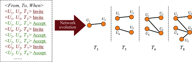
Figure 1: Data format and evolution of OSN Wealink.

3.2 Preferential Linking

Like some other OSNs the degree distribution of Wealink shows power-law feature. This kind of distribution can be produced through linear PA, as revealed by BA model. In addition to the dynamics that is due to new users joining the network (generally by creating a new account) and making friends with the old users, there is also the dynamics that results from active users interacting with each other. In real scenario of network growth when new users establish friend relationship with old users, or new ties are established between old users, the old users with large degrees are all likely to be preferentially selected. In this subsection we will give evidence supporting these hypotheses.

Since many OSNs are consequence of bilateral decisions of a pair of users, not of their unilateral decisions, to test the preference feature for different types of link establishment, we separate PL into three aspects: preferential acceptance, preferential creation, and PA. Preferential acceptance implies that, the larger an old user’s degree is, the more likely she/he will be selected as friends by the other old users. Preferential creation implies that, the larger an old user’s degree is, the more likely her/his link invitations will be accepted by the other old users. The meaning of PA remains unchanged, i.e. new users tend to attach to already popular old users with large degrees.

Let $k_{i}$ be the degree of user $i$. The probability that user $i$ with degree $k_{i}$ is chosen can be expressed as

$$\prod(k_{i})=\frac{{k_{i}^{\beta}}}{{\sum\nolimits_{j}{k_{j}^{\beta}}}}.$$ (1)

We can compute the probability $\Pi(k)$ that an old user of degree $k$ is chosen, and it is normalized by the number of users of degree $k$ that exist just before this step:

$$\prod(k)=\frac{{\sum\nolimits_{t}{\left[{e_{t}=v\wedge k_{v}(t-1)=k}\right]}}}{{\sum\nolimits_{t}{\left|{\left\{{u:k_{u}(t-1)=k}\right\}}\right|}}}\propto k^{\beta},$$ (2)

where $e_{t}=v\wedge k_{v}(t-1)=k$ represents that at time $t$ the old user whose degree is $k$ at time $t-1$ is chosen. We use $[\cdot]$ to denote a predicate (which takes a value of 1 if the expression is true, else 0). Generally, $\Pi(k)$ has significant fluctuations, particularly for large $k$. To reduce the noise level, instead of $\Pi(k)$, we study the cumulative function:

$$\kappa(k)=\int_{0}^{k}{\prod(k){\rm{d}}k}\propto k^{\beta+1}=k^{\alpha}.$$ (3)

Fig. 2 shows the relation between degree $k$ of users and preference metric $\kappa$. Least squares linear regression gives $\alpha=1.93\pm 0.01(R^{2}=0.99)$ for preferential creation, $\alpha=1.97\pm 0.01(R^{2}=0.98)$ for PA and $\alpha=2.06\pm 0.01(R^{2}=0.99)$ for preferential acceptance. All are with significance level $p<2.2\times 10^{-16}$. Thus $\beta\approx 1$ indicating linear preference.

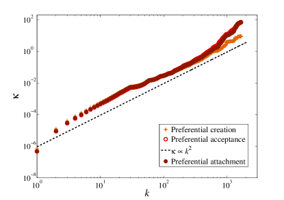
Figure 2: Preference characteristics in the evolution of Wealink.

3.3 Model

Like other OSNs the evolution of Wealink includes two processes. The first one is that a new user joins in the network and establishes friend relation with an old user already present in the network. The second one is that a friend relation is established between two old users. Certainly there exists the case that a tie forms between two new users; however the situation is rare in real world and can be neglected.

Based on the linear preference we bring forward the following network model. Starting with a small connected network with $m_{0}$ users, at every time step, there are two alternatives:

$A$. With probability $p$, we add a new user with one edge that will be connected to the user already present in the network. The probability that the new user will be connected to old user $i$ with degree $k_{i}$ is $\Pi({k_{i}})={k_{i}}/\sum\nolimits_{j}{{k_{j}}}$.

$B$. With probability $q=1-p$, we add one new edge connecting the old users. The two endpoints of the edge are also chosen according to linear preference.

After $t$ time steps the model leads to a network with mean number of users $N(t)=m_{0}+pt$. For large $t$, $N\approx pt$ and the total degree of the network $k_{{\rm{all}}}(t)\approx 2t$. Applying mean-field approach for user $i$, we obtain

$$\frac{{\partial{k_{i}}}}{{\partial t}}=p\frac{{{k_{i}}}}{{\sum\nolimits_{j}{{k_{j}}}}}+2q\frac{{{k_{i}}}}{{\sum\nolimits_{j}{{k_{j}}}}}=\frac{{p+2q}}{{2t}}{k_{i}}.$$ (4)

The solution of Eq. (4) with the initial condition $k_{i}(t_{i})=1$ is

$${k_{i}}={(t/{t_{i}})^{\frac{{p+2q}}{2}}}.$$ (5)

Thus

$$P({k_{i}}<k)=P({t_{i}}>{k^{-\frac{2}{{p+2q}}}}\cdot t).$$ (6)

The probability density of $t_{i}$ for large $t$ is

$${P_{i}}({t_{i}})={1\mathord{\left/{\vphantom{1{\left({{m_{0}}+tp}\right)}}}\right.\kern-1.2pt}{\left({{m_{0}}+tp}\right)}}\approx 1/(tp).$$ (7)

From Eq. (6) we obtain

$$P({k_{i}}<k)=1-P({t_{i}}\leq{k^{-\frac{2}{{p+2q}}}}\cdot t)=1-{p^{-1}}\cdot{k^{-\frac{2}{{p+2q}}}}.$$ (8)

Thus the probability density for $P(k)$ is

$$P(k)=\frac{{\partial P({k_{i}}<k)}}{{\partial k}}\propto k^{-\frac{{4-p}}{{2-p}}}.$$ (9)

The exponent $\gamma\in(2,3]$ and when $p=1$ the model is reduced to BA model.

According to empirical data, we obtain $p={\rm{0}}{\rm{.7941}}$ and $q=0.1939$. The links created between two new users are few and thus can be negligible. Based on the parameters and Eq. (9), we obtain $P(k)\propto k^{-2.67}$. Fig. 3 shows the numerical result which is obtained by averaging over 10 independent realizations with $p={\rm{0}}{\rm{.7941}}$ and the same number of users as Wealink. Its degree exponent 2.62 agrees well with the predicted value of 2.67. Fig. 3 also presents the complementary cumulative degree distribution of Wealink. We fit the network data with power-law model utilizing Maximum Likelihood Estimate method and obtain $\gamma=2.91$. The predicted value of the degree exponent 2.67 of the model achieves proper agreement with the real value 2.91. We also compute $p$-value for the estimated power-law fit to the network implementing the Kolmogorov-Smirnov test and obtain $p=0.704$ [32]. We choose threshold 0.1, and thus the power-law fit is a good match to the degree distribution of $Wealink$.

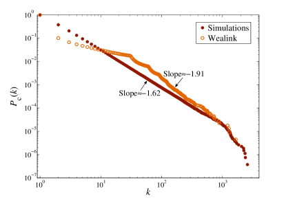
Figure 3: The complementary cumulative degree distributions of $Wealink$ and the networks obtained by numerical simulations.

In real world different from the ideal model, the probability $p$ cannot be stationary during the evolution of OSNs. In some stage $p$ can be very large while in another stage $p$ can be very small, which can lead to the difference between real exponent and predicted one. Fig. 4 shows the evolution of $p$ and $q$, and demonstrates the fact. As a guide we also indicate the positions of $p=0.7941$ and $q=0.1939$.

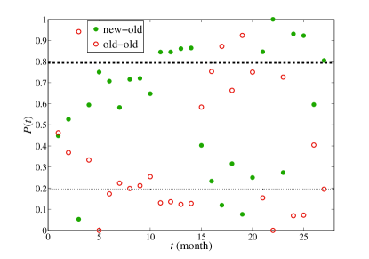
Figure 4: Evolution of the fraction of two kinds of edges. Dashed line indicates $p=0.7941$ while dotted line $q=0.1939$.

4 Generalized Model

In ONSs new users are constantly joining the social networks, and create edges towards already present users. Very few users leave the network, and very few edges disappear between users which remain in the network. Edges on the other hand are created between already present users. Besides in the evolution of real OSNs, new users or edges are added into networks one by one, and previous empirical researches have also shown that in OSNs most preference exponent $\beta\leq 1$. Thus we bring forward the following general network model. Still starting with a small connected network with $m_{0}$ users, however at every time step, there are another two alternatives:

$A$. With probability $p$, we add a new user with one edge that will be connected to the user already present in the network. The probability that the new user will be connected to old user $a$ with degree $k_{a}$ is $\Pi({k_{a}})=k_{a}^{\alpha}/\sum\nolimits_{j}{k_{j}^{\alpha}}$, where $0\leq\alpha\leq 1$.

$B$. With probability $q=1-p$, we add one new edge connecting the old users. One endpoint $b$ is chosen according to $\Pi({k_{b}})=k_{b}^{\beta}/\sum\nolimits_{j}{k_{j}^{\beta}}$ while another endpoint $c$ is chosen according to $\Pi({k_{c}})=k_{c}^{\gamma}/\sum\nolimits_{j}{k_{j}^{\gamma}}$, , where $0\leq\beta,\gamma\leq 1$.

Thus

$$\frac{{\partial{k_{i}}}}{{\partial t}}=p\frac{{k_{i}^{\alpha}}}{{\sum\nolimits_{j}{k_{j}^{\alpha}}}}+q\frac{{k_{i}^{\beta}}}{{\sum\nolimits_{j}{k_{j}^{\beta}}}}+q\frac{{k_{i}^{\gamma}}}{{\sum\nolimits_{j}{k_{j}^{\gamma}}}},$$ (10)

where $0<p,q<1$.

According to

$$\left\{\begin{array}[]{l}\sum\nolimits_{j}{k_{j}^{0}=pt}\\ \sum\nolimits_{j}{k_{j}^{1}=2t}\\ \end{array}\right.,$$ (11)

when $0<\alpha<1$, $\sum\nolimits_{j}{k_{j}^{\alpha}=ut}$ where $p<u<2$.

As users $a$, $b$ and $c$ can be chosen according to any one of three rules–random attachment, linear PL and sublinear PL, there are 27 different scenarios for the evolution of ONSs.

First we consider the situations where only linear PL or random attachment exists, i.e. $\alpha,\beta,\gamma=1$ or 0, and there are totally eight scenarios which can be divided into six cases. Utilizing the similar approach in Sec. 3, we get all their degree distributions which have been summarized in Tab. 1. It is not surprising that for case I linear PL will result in power-law distribution, and for case VI random attachment will lead to exponential distribution. However it is interesting that for the other cases, the combination of linear PL component and randomized attachment component also will generate networks with approximatively power-law distribution. Besides according to the variation range of degree exponent in Tab. 1, obviously the introduction of randomized attachment can enhance the homogeneity of network structure.

Table 1: The evolution of $k_{i}$ and corresponding $P(k)$ when only linear PL or random attachment exists.

• Case	$a$	$b$	$c$	$\partial{k_{i}}/\partial t$	$P(k)$
  I	Linear	Linear	Linear	$\frac{{p+2q}}{{2t}}{k_{i}}$	$\propto k^{-\frac{{4-p}}{{2-p}}}$
  II	Linear	Linear	Random	$\frac{{{k_{i}}}}{{2t}}+\frac{q}{{pt}}$	$\propto(kp+2q)^{-3}$
  	Linear	Random	Linear
  III	Linear	Random	Random	$\frac{{p{k_{i}}}}{{2t}}+\frac{{2q}}{{pt}}$	$\propto{(k{p^{2}}+4q)^{-\left({1+\frac{2}{p}}\right)}}$
  IV	Random	Linear	Linear	$\frac{1}{t}+\frac{{q{k_{i}}}}{t}$	$\propto{(kq+1)^{-\left({1+\frac{1}{q}}\right)}}$
  V	Random	Linear	Random	$\frac{1}{{pt}}+\frac{{q{k_{i}}}}{{2t}}$	$\propto{(kpq+2)^{-\left({1+\frac{2}{q}}\right)}}$
  	Random	Random	Linear
  VI	Random	Random	Random	$\frac{{p+2q}}{{pt}}$	$\propto{{\rm{e}}^{-\frac{{pk}}{{p+2q}}}}$

When sublinear PL exists, there are 19 different scenarios for the evolution of $k_{i}$ which can be divided into 12 cases and are shown in Tab. 2. According to Lipschitz conditions there are unique solutions to $k_{i}$.

Table 2: The evolution of $k_{i}$ when sublinear PL exists. $0<\alpha,\beta,\gamma<1$ and $p<u,v,w<2$.

• Case	$a$	$b$	$c$	$\partial{k_{i}}/\partial t$
  I	Sublinear	Linear	Linear	$\frac{{pk_{i}^{\alpha}}}{{ut}}+\frac{{q{k_{i}}}}{t}$
  II	Linear	Sublinear	Linear	$\frac{{qk_{i}^{\beta}}}{{vt}}+\frac{{{k_{i}}}}{{2t}}$
  	Linear	Linear	Sublinear
  III	Sublinear	Sublinear	Sublinear	$\frac{{pk_{i}^{\alpha}}}{{ut}}+\frac{{qk_{i}^{\beta}}}{{vt}}+\frac{{qk_{i}^{\gamma}}}{{wt}}$
  IV	Random	Sublinear	Sublinear	$\frac{1}{t}+\frac{{qk_{i}^{\beta}}}{{vt}}+\frac{{qk_{i}^{\gamma}}}{{wt}}$
  V	Sublinear	Sublinear	Random	$\frac{{pk_{i}^{\alpha}}}{{ut}}+\frac{{qk_{i}^{\beta}}}{{vt}}+\frac{q}{{pt}}$
  	Sublinear	Random	Sublinear
  VI	Linear	Sublinear	Sublinear	$\frac{{p{k_{i}}}}{{2t}}+\frac{{qk_{i}^{\beta}}}{{vt}}+\frac{{qk_{i}^{\gamma}}}{{wt}}$
  VII	Sublinear	Sublinear	Linear	$\frac{{pk_{i}^{\alpha}}}{{ut}}+\frac{{qk_{i}^{\beta}}}{{vt}}+\frac{{q{k_{i}}}}{{2t}}$
  	Sublinear	Linear	Sublinear
  VIII	Random	Sublinear	Random	$\frac{1}{t}+\frac{{qk_{i}^{\beta}}}{{vt}}+\frac{q}{{pt}}$
  	Random	Random	Sublinear
  IX	Sublinear	Random	Random	$\frac{{pk_{i}^{\alpha}}}{{ut}}+\frac{{2q}}{{pt}}$
  X	Linear	Sublinear	Random	$\frac{{p{k_{i}}}}{{2t}}+\frac{{qk_{i}^{\beta}}}{{vt}}+\frac{q}{{pt}}$
  	Linear	Random	Sublinear
  XI	Random	Sublinear	Linear	$\frac{1}{t}+\frac{{qk_{i}^{\beta}}}{{vt}}+\frac{{q{k_{i}}}}{{2t}}$
  	Random	Linear	Sublinear
  XII	Sublinear	Linear	Random	$\frac{{pk_{i}^{\alpha}}}{{ut}}+\frac{q}{{pt}}+\frac{{q{k_{i}}}}{{2t}}$
  	Sublinear	Random	Linear

For case I we obtain

$$\frac{{\partial k_{i}}}{{\partial t}}-\frac{q}{t}k_{i}=\frac{p}{{ut}}k_{i}^{\alpha},$$ (12)

which is Bernoulli’s differential equation. Let $z=k_{i}^{1-\alpha}$, thus

$$\frac{{\partial z}}{{\partial t}}-\frac{q}{t}(1-\alpha)z=(1-\alpha)\frac{p}{{ut}}.$$ (13)

Therefore

$$z = {\rm{e}}^{{\rm{-}}\int{\frac{{(\alpha-1)q}}{t}{\rm{d}}t}}\left({c+\int{\frac{{p(1-\alpha)}}{{ut}}{\rm{e}}^{\int{\frac{{(\alpha-1)q}}{t}{\rm{d}}t}}{\rm{d}}t}}\right)$$ (14)

$$= c_{1}t^{(1-\alpha)q}-\frac{p}{{uq}},$$

where $c$ and $c_{1}$ are constants. Thus

$$k_{i}=\left[{c_{1}t^{(1-\alpha)q}-\frac{p}{{uq}}}\right]^{\frac{1}{{1-\alpha}}}.$$ (15)

According to initial value $k_{i}(t_{i})=1$, we obtain

$$k_{i}=\left[{\left({1+\frac{p}{{uq}}}\right)\left({\frac{t}{{t_{i}}}}\right)^{(1-\alpha)q}-\frac{p}{{uq}}}\right]^{\frac{1}{{1-\alpha}}}.$$ (16)

Accordingly

$$P(k)\propto\left({uqk^{1-\alpha}+p}\right)^{-\left[{1+\frac{1}{{(1-\alpha)q}}}\right]},$$ (17)

and for large $k$, $P(k)\propto k^{-\left({1-\alpha+\frac{1}{q}}\right)}$.

Similarly for case II we obtain

$$P(k)\propto\left({\frac{1}{2}vk^{1-\alpha}+q}\right)^{-\left({\frac{2}{{1-\alpha}}+1}\right)},$$ (18)

and for large $k$, $P(k)\propto k^{-(3-\alpha)}$.

For case III when $\alpha=\beta=\gamma$

$$\frac{{\partial k_{i}}}{{\partial t}}=\frac{{(1+q)k_{i}^{\alpha}}}{{ut}},$$ (19)

thus

$$k_{i}=\left[{1+\frac{{(1-\alpha)(1+q)\ln\frac{t}{{t_{i}}}}}{u}}\right]^{\frac{1}{{1-\alpha}}}.$$ (20)

Accordingly

$$P(k)\propto k^{-\alpha}\exp\left[{\frac{{-uk^{1-\alpha}}}{{(1-\alpha)(1+q)}}}\right],$$ (21)

which is stretched exponential distribution.

For case VI when $\beta=\gamma$, we have

$$\frac{{\partial k_{i}}}{{\partial t}}=\frac{{pk_{i}}}{{2t}}+\frac{{2qk_{i}^{\beta}}}{{vt}}.$$ (22)

According to the derivation in case I, we obtain

$$P(k)\propto\left({\frac{{vp}}{2}k^{1-\beta}+2q}\right)^{-\left[{\frac{2}{{p(1-\beta)}}+1}\right]},$$ (23)

and for large $k$, $P(k)\propto k^{-\left({\frac{2}{p}+1-\beta}\right)}$.

For case VII when $\alpha=\beta$, we have

$$\frac{{\partial k_{i}}}{{\partial t}}=\frac{{k_{i}^{\alpha}}}{{ut}}+\frac{{qk_{i}}}{{2t}}.$$ (24)

Similarly we obtain

$$P(k)\propto\left({\frac{{uq}}{2}k^{1-\alpha}+1}\right)^{-\left[{\frac{2}{{(1-\alpha)q}}+1}\right]},$$ (25)

and for large $k$, $P(k)\propto k^{-\left({\frac{2}{q}+1-\alpha}\right)}$.

The situations in which we can obtain analytical solutions with mean-field method have been shown in Fig. 5. Bold solid lines mark the situations with power-law degree distribution while bold dashed line indicates the situations with stretched exponential distribution except the two endpoints (exponential for (0, 0, 0) while power law for (1, 1, 1)). Using the common approaches, including mean-field, rate equation and master equation, we cannot obtain all analytical solutions to 27 different scenarios.

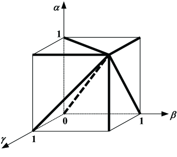
Figure 5: The situations which are solvable with mean-field method.

We notice that Eq. (10) can be expressed as

$$\frac{{\partial{k_{i}}}}{{\partial t}}=\left({ak_{i}^{\alpha}+bk_{i}^{\beta}+ck_{i}^{\gamma}}\right)\frac{1}{t},$$ (26)

where $a$, $b$ and $c$ are constants. Namely

$$\int\limits_{k_{i}(t_{i})}^{k_{i}(t)}{\frac{{{\rm{d}}k_{i}}}{{(ak_{i}^{\alpha}+bk_{i}^{\beta}+ck_{i}^{\gamma})}}}=\ln\frac{t}{{t_{i}}}.$$ (27)

When $t_{j}<t_{i}$,

$$\int_{k_{i}(t_{i})}^{k_{i}(t)}{\frac{{{\rm{d}}x}}{{ax^{\alpha}+bx^{\beta}+cx^{\gamma}}}}<\int_{k_{j}(t_{j})}^{k_{j}(t)}{\frac{{{\rm{d}}x}}{{ax^{\alpha}+bx^{\beta}+cx^{\gamma}}}}.$$ (28)

Since $k_{i}(t_{i})=k_{j}(t_{j})=1$,

$$\int_{1}^{k_{i}(t)}{\frac{{{\rm{d}}x}}{{ax^{\alpha}+bx^{\beta}+cx^{\gamma}}}}<\int_{1}^{k_{j}(t)}{\frac{{{\rm{d}}x}}{{ax^{\alpha}+bx^{\beta}+cx^{\gamma}}}}.$$ (29)

Thus $k_{i}(t)<k_{j}(t)$, i.e. the degrees of the users which appeared in networks before user $i$ are almost everywhere larger than $k_{i}$. Thus the complementary cumulative degree distribution of networks can be written as

$$P_{\rm{c}}(k)\propto\frac{{N(t_{i})}}{{N(t)}}\approx\frac{{t_{i}}}{t}.$$ (30)

According to Eqs. (27) and (30), we obtain

$${P_{\rm{c}}}(k)\propto{{\rm{e}}^{-\int_{1}^{k}{\frac{{{\rm{d}}{k_{i}}}}{{ak_{i}^{\alpha}+bk_{i}^{\beta}+ck_{i}^{\gamma}}}}}}.$$ (31)

Let $n_{1}$, $n_{2}$ and $n_{3}$ be non-negative integers, $m$ be positive integer, and $\alpha=n_{1}/m$, $\beta=n_{2}/m$ and $\gamma=n_{3}/m$. Further let $s=k_{i}^{1/m}$ then

$$\int_{1}^{k}{\frac{{{\rm{d}}k_{i}}}{{ak_{i}^{\alpha}+bk_{i}^{\beta}+ck_{i}^{\gamma}}}}=\int_{1}^{k^{1/m}}{\frac{{ms^{m-1}{\rm{d}}s}}{{as^{n_{1}}+bs^{n_{2}}+cs^{n_{3}}}}}.$$ (32)

Suppose that $n_{1}>n_{2}>n_{3}$ and let

$$\frac{{m{s^{m-1}}}}{{a{s^{{n_{1}}}}+b{s^{{n_{2}}}}+c{s^{{n_{3}}}}}}=\frac{{m{s^{m-1-n_{3}}}}}{{a{s^{{n_{1}-n_{3}}}}+b{s^{{n_{2}-n_{3}}}}+c}}=P(s)+\frac{{\hat{P}(s)}}{{Q(s)}},$$ (33)

where $P(s)$ and $\hat{P}(s)$ are polynomials with ${\rm{deg\,}}\hat{P}<{\rm{deg\,}}Q$. Furthermore suppose that the polynomial $Q(s)$ has $l$ distinct complex conjugate pairs of roots ${\eta_{1}}\pm i{\mu_{1}}$, $\ldots$, ${\eta_{l}}\pm i{\mu_{l}}$ and $k$ distinct real roots $\lambda_{1}$, $\ldots$, $\lambda_{k}$, then we have

$$Q(s)={\prod\limits_{i=1}^{l}{\left[{{{\left({s-{\eta_{i}}}\right)}^{2}}+\mu_{i}^{2}}\right]}^{{m_{i}}}}\prod\limits_{i=1}^{k}{{{\left({s-{\lambda_{i}}}\right)}^{{n_{i}}}}},$$ (34)

where $m_{i}$ and $n_{i}$ denote the multiplicities of the roots. For $\hat{P}(s)/Q(s)$ there exist real constants $A_{ij}$, $B_{ij}$ and $C_{ij}$ such that

$$\frac{{\hat{P}(s)}}{{Q(s)}}{\rm{=}}\sum\limits_{i{\rm{=}}1}^{l}{\sum\limits_{j{\rm{=}}1}^{{m_{i}}}{\frac{{{A_{ij}}{\rm{+}}{B_{ij}}s}}{{{{\left[{{{\left({s{\rm{-}}{\eta_{i}}}\right)}^{2}}{\rm{+}}\mu_{i}^{2}}\right]}^{j}}}}}}{\rm{+}}\sum\limits_{i{\rm{=}}1}^{k}{\sum\limits_{j{\rm{=}}1}^{{n_{i}}}{\frac{{{C_{ij}}}}{{{{\left({s{\rm{-}}{\lambda_{i}}}\right)}^{j}}}}}}.$$ (35)

The second term of the right-hand side of Eq. (35) can easily be integrated. For the first term when $j=1$ we have

$$\int{\frac{{A{\rm{+}}Bs}}{{{{\left({s{\rm{-}}\eta}\right)}^{2}}{\rm{+}}{\mu^{2}}}}}{\rm{d}}s{\rm{=}}\frac{B}{2}\ln\left[{{{\left({s{\rm{-}}\eta}\right)}^{2}}{\rm{+}}{\mu^{2}}}\right]{\rm{+}}\frac{{A{\rm{+}}B\eta}}{\mu}\arctan\left({\frac{{s{\rm{-}}\eta}}{\mu}}\right),$$ (36)

and when $j>1$

$$\int{\frac{{A+Bs}}{{{{\left[{{{\left({s-\eta}\right)}^{2}}+{\mu^{2}}}\right]}^{j}}}}}{\rm{d}}s=\frac{{-B}}{{2(j-1){{\left[{{{\left({s-\eta}\right)}^{2}}+{\mu^{2}}}\right]}^{j-1}}}}+\frac{{A+B\eta}}{{{\mu^{2j-1}}}}{J_{j}}\left({\frac{{s-\eta}}{\mu}}\right),$$ (37)

where $J_{1}(z)=\arctan z$ and

$${J_{j+1}}(z)=\frac{z}{{2j{{\left({{z^{2}}+1}\right)}^{j}}}}+\frac{{2j-1}}{{2j}}{J_{j}}(z).$$ (38)

Thus according to Eqs. (33)-(38), the primitive function of Eq. (33) can only be the sum of rational functions, logarithmic functions and inverse tangent functions, and for all scenarios in the generalized model, we can analytically obtain their degree distributions though the expressions can be complex in most scenarios.

In cases III–XII in Tab. 2, for some special parameters of $\alpha$, $\beta$ or $\gamma$, we can easily obtain the solutions to $P_{c}(k)$. For example in case VIII, when $\beta=1/3$

$${P_{\rm{c}}}(k) \propto \exp\left[{-\int_{{1}}^{{k^{1/3}}}{\left({\frac{{3vs}}{q}-\frac{{3{v^{2}}}}{{{q^{2}}p}}+\frac{{{{3{v^{3}}}\mathord{\left/{\vphantom{{3{v^{3}}}{\left({{q^{2}}p}\right)}}}\right.\kern-1.2pt}{\left({{q^{2}}p}\right)}}}}{{qps+v}}}\right){\rm{d}}s}}\right]$$ (39)

$$= {\left({pq{k^{1/3}}+v}\right)^{-\frac{{3{v^{3}}}}{{{p^{2}}{q^{3}}}}}}\exp\left({-\frac{{3v{k^{2/3}}}}{{2q}}+\frac{{3{v^{2}}{k^{1/3}}}}{{{q^{2}}p}}}\right).$$

Although quite controversial online friendship is thought to be vitally important for the well-being and social capital of people [33, 34]. We use Gini coefficient to quantify the inequality of the degrees of users [35]. Fig. 6 shows the numerical result which is obtained by averaging over 20 independent realizations. For Eq. (10) when $\alpha=0.2$, the corresponding numerical result for $0\leq\beta,\gamma\leq 1$ is shown in Fig. 6(a). As expected along minor diagonal symmetrical pattern emerges. When $\gamma=0.2$ the corresponding numerical result for $0\leq\alpha,\beta\leq 1$ is shown in Fig. 6(b). The numerical simulations include all cases in Tab. 2. It is evident that larger preference exponent will result in greater inequality of the degrees of users and the emergence of hubs, and thus larger Gini coefficient. Besides we find that from randomized attachment to PL there is a clear jump for network heterogeneity, which implies that PL can significantly enhance the inequality of individual social capital.

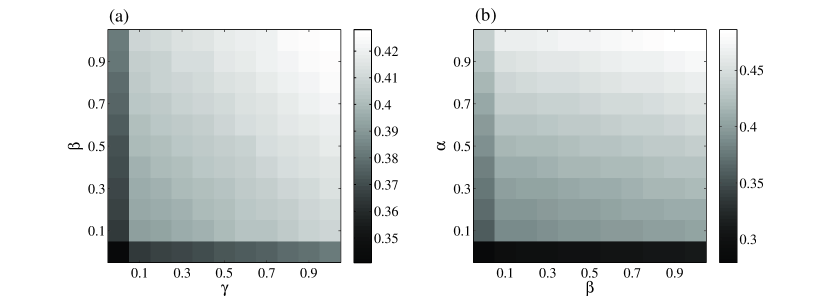
Figure 6: Gini coefficients of networks obtained by numerical simulations with $p=0.8$ and $N=10^{4}$.

5 Conclusion and Discussion

In summary, we empirically study PL in an evolving OSN, find and validate the existence of linear preference. We propose an analyzable model which reproduces the growth process of the OSN. Furthermore we bring forward a generalized theory of PL and obtain the unified analytical solutions for diverse preference cases with a more general approach.

Why people prefer to attach their links to others who have more links? Obviously in real life we make friends with someone not because she/he has many friends but she/he possesses some quality we expect and is also willing to make friends with us. Thus large degree predicates that the actor is a worthful and trustworthy person and making friends with her/him will benefit us. Many researches have found a positive association between an actor’s degree and that actor’s goal achievement, including creativity, job attainment, professional advancement, political influence and prestige. Thus a user’s degree is a stand-in for her/his true fitness since direct performance data are costly to gather before the relationship is made. PL purportedly occurs because actors looking for new connections use an actor’s degree as a proxy for her/his fitness. A profile owner with many friends will be judged as more popular than a profile owner with few friends [36].

Kim and Jo proposed several interesting models and explained PA as rational equilibrium behavior [37]. In fact people are not certain of the value that they can obtain from forming a link with someone. A person has an incentive to form a link with another who has many links because the number of her/his links can convey some information about her/his value; in an economic sense, the number of links can be a signal of the value of the person, i.e. the observable degree contains some information about her/his unobservable value. From the perspective of economics, if the return obtained by interacting with someone is greater than the cost, we like and are willing to continue to maintain this relationship, especially when the benefit in this relationship outweighs the other possible relationship. The users with large degrees precisely are the persons from whom we can expect to get more profit.

PL is widely used as an evolution mechanism of networks. However it is hard to believe that any individual can get global information and shape the network architecture based on it. Li et al. found that the global PA can emerge from the local interaction models, including the distance-dependent PA evolving model, the acquaintance network model and the connecting nearest-neighbor model [38]. In fact Aiello et al. have found that many users join aNobii by creating links to pairs of already connected users [29].

As shown in Fig. 4, the probabilities $p$ and $q$ are time-variant and cannot be stationary during the real evolution of OSNs. Besides the activity of users can weaken over time [9]. There exists a memory kernel which dominates the decline of users’ activity and might be highly skewed, for example obeying power law [39]. Thus a more realistic model can be that $p$, $q$, $\alpha$, $\beta$ and $\gamma$ in Eq. (10) are all time-dependent.

Why two people become friends? This question has been widely and intensively studied in social psychology. Except PL there are diverse mechanisms which can lead to the formation of dyadic ties, such as homophily, relational or propinquity mechanisms and physical attractiveness, and they are intimately interwoven in the evolution of real social networks and have been found working in the formation of OSNs [16, 27]. For example homophily has been found in Facebook [40], Microsoft Messenger [41], LiveJournal [42], aNobii [29], MySpace [43] and online dating sites [44, 45]. For relational mechanism, the connecting nearest-neighbor model has been proposed to explain the mechanism [46] and empirical research has shown that this mechanism is at work in aNobii [29]. Besides although the Internet transcends some of the limitations of physical space, proximity still matters in OSNs [47, 48], especially for online dating in which a face-to-face relationship is the goal. PL can account for the degree distribution of OSNs; however it cannot explain the other structural or sociological characteristics of the networks. A deeper understanding of these mechanisms can allow us to better model and predict structure and dynamics of OSNs [49-51]. Krivitsky et al. made an effort towards the goal [52]. They proposed a latent cluster random effects model to represent degree distributions, clustering, and homophily in social networks, however the model is essentially statistical not growing [53].

Most conclusions of the article are theoretical, and need to be validated by empirical network datasets. Because of the diversity of purposes of SNSs, there can exist disparate mechanisms dominating the formation and evolution of OSNs. To the OSNs for general users, old users can incline to associate with others similar to themselves and homophily can dominate. While to the OSNs for professionals, old users can prefer to associate with the celebrities in the same vocation because personal success in occupation may benefit from the communication with them. Besides the relative importance of different mechanisms is also different in different growth stages of OSNs. In the beginning stage users may incline to establish friendship relations with the users who are their friends in real life, while in the later stage users may prefer to make friends with the users whom they do not know in real life while they are interested in, which can result in the transition from degree assortativity to disassortativity [54]. Consider the diversity of users and the fact that network growth mechanisms tend to be correlated with each other, for such multidimensional diversity and complexity, we could only simulate or reproduce one or several of the network characteristics. Incorporating more social psychological and economic viewpoints and approaches into the modeling study of OSNs is beneficial to better understanding the formation of dyadic ties, which will be a possible future research direction though the analyses would be much more complex in that setting.

References

References

- [1] Moreno J L, 1934, Who Shall Survive (Washington, DC: Nerv. Ment. Dis.)
- [2] Jennings H, 1943, Leadership and Isolation: A Study of Personality in Interpersonal Relations (New York: Longmans)
- [3] Borgatti S P and Everett M G, 2006 Social Networks 28 466
- [4] Liljeros F, Edling C R, Amaral L A N, Stanley H E and Aberg Y, 2001 Nature 411 907
- [5] Albert R and Barabási A L, 2002 Rev. Mod. Phys. 74 47
- [6] Lazer D, Pentland A, Adamic L, Aral S, Barabási A L, Brewer D, Christakis N, Contractor N, Fowler J, Gutmann M, Jebara T, King G, Macy M, Roy D and Alstyne M V, 2009 Science 323 721
- [7] boyd d m and Ellison N B, 2007 Journal of Computer-Mediated Communication 13 210
- [8] Lewis K, Kaufman J, Gonzalez M, Wimmer A and Christakis N, 2008 Social Networks 30 330
- [9] Zhao X, Sala A, Wilson C, Wang X, Gaito S, Zheng H and Zhao B Y, Multi-scale dynamics in a massive online social network, 2012 Proceedings of the 2012 ACM conference on Internet measurement conference pp 171-184
- [10] Ahn Y Y, Han S, Kwak H, Moon S and Jeong H, Analysis of topological characteristics of huge online social networking services, 2007 Proceedings of the 16th international conference on World Wide Web pp 835-844
- [11] Wilkinson D and Thelwall M, 2010 J. Am. Soc. Inf. Sci. Technol. 61 2311
- [12] Mislove A, Marcon M, Gummadi K P, Druschel P and Bhattacharjee B, Measurement and analysis of online social networks, 2007 Proceedings of the 7th ACM SIGCOMM conference on Internet measurement pp 29-42
- [13] Gong N Z, Xu W, Huang L, Mittal P, Stefanov E, Sekar V and Song D, Evolution of social-attribute networks: Measurements, modeling, and implications using Google+, 2012 Proceedings of the 2012 ACM conference on Internet measurement conference pp 131-144
- [14] Ugander J, Karrer B, Backstrom L and Marlow C, 2011 arXiv: 1111.4503
- [15] Diprete T A and Eirich G M, 2006 Annu. Rev. Sociol. 32 271
- [16] Rivera M T, Soderstrom S B and Uzzi B, 2010 Annu. Rev. Sociol. 36 91
- [17] Opsahl T and Hogan B, 2010 arXiv: 1010.2141
- [18] Traud A L, Mucha P J and Porter M A, 2012 Physica A 391 4165
- [19] Barabási A L and Albert R, 1999 Science 286 509
- [20] Krapivsky P L, Rodgers G J and Redner S, 2001 Phys. Rev. Lett. 86 5401
- [21] Newman M E J, 2001 Phys. Rev. E 64 025102
- [22] Jeong H, Néda Z and Barabási A L, 2003 Europhys. Lett. 61 567.
- [23] Peltomäki M and Alava M, 2006 J. Stat. Mech. 2006 P01010
- [24] de Blasio B F, Svensson A and Liljeros F, 2007 Proc. Natl Acad. Sci. USA 104 10762
- [25] Mislove A, Koppula H S, Gummadi K P, Druschel P and Bhattacharjee B, Growth of the Flickr social network, 2008 Proceedings of the first workshop on Online social networks pp 25-30
- [26] Leskovec J, Backstrom L, Kumar R and Tomkins A, Microscopic evolution of social networks, 2008 Proceedings of the 14th ACM SIGKDD international conference on Knowledge discovery and data mining pp 462-470
- [27] Garg S, Gupta T, Carlsson N and Mahanti A, Evolution of an online social aggregation network: an empirical study, 2009 Proceedings of the 9th ACMSIGCOMMconference on Internet measurement conference pp 315-321
- [28] Szell M and Thurner S, 2010 Social Networks 32 313
- [29] Aiello L M, Barrat A, Cattuto C, Ruffo G and Schifanella R, Link creation and profile alignment in the aNobii social network, 2010 Proceedings of the 2010 IEEE Second International Conference on Social Computing pp 249-256
- [30] Rocha L E C, Liljeros F and Holme P, 2010 Proc. Natl Acad. Sci. USA 107 5706
- [31] Viswanath B, Mislove A, Cha M and Gummadi K P, On the evolution of user interaction in Facebook, 2009 Proceedings of the 2nd ACM workshop on Online social networks pp 37-42
- [32] Clauset A, Shalizi C and Newman M, 2009 SIAM Rev. 51 661
- [33] Dunbar R I M, 2012 Phil. Trans. R. Soc. B 367 2192
- [34] Valenzuela S, Park N and Kee K F, 2009 Journal of Computer-Mediated Communication 14 875
- [35] Stirling A, 2007 J. R. Soc. Interface 4 707
- [36] Utz S, 2010 Journal of Computer-Mediated Communication 15 314
- [37] Kim J Y and Jo H H, 2010 Journal of Evolutionary Economics 20 375
- [38] Li M, Gao L, Fan Y, Wu J and Di Z, 2010 New J. Phys. 12 043029
- [39] Cattuto C, Loreto V and Pietronero L, 2007 Proc. Natl Acad. Sci. USA 104 1461
- [40] Wimmer A and Lewis K, 2010 American Journal of Sociology 116 583
- [41] Leskovec J and Horvitz E, Planetary-scale views on a large instant-messaging network, 2008 Proceedings of the 17th international conference on World Wide Web pp 915-924
- [42] Lauw H, Shafer J C, Agrawal R and Ntoulas A, 2010 IEEE Internet Computing 14 15
- [43] Thelwall M, 2009 J. Am. Soc. Inf. Sci. Technol. 60 219
- [44] Fiore A T and Donath J S, Homophily in online dating: when do you like someone like yourself? 2005 CHI 05 extended abstracts on Human factors in computing systems pp 1371-1374
- [45] Skopek J, Schulz F and Blossfeld H P, 2011 Eur. Sociol. Rev. 27 180
- [46] Vázquez A, 2003 Phys. Rev. E 67 056104
- [47] Liben-Nowell D, Novak J, Kumar R, Raghavan P and Tomkins A, 2005 Proc. Natl Acad. Sci. USA 102 11623
- [48] Amichai-Hamburger Y, Kingsbury M and Schneider B H, 2013 Computers in Human Behavior 29 33
- [49] Liben-Nowell D and Kleinberg J, 2007 J. Am. Soc. Inf. Sci. Technol. 58 1019
- [50] Aiello L M, Barrat A, Schifanella R, Cattuto C, Markines B and Menczer F, 2012 ACM Trans. Web 6 2 9
- [51] Lü L and Zhou T, 2011 Physica A 390 1150
- [52] Krivitsky P N, Handcock M S, Raftery A E and Hoff P D, 2009 Social Networks 31 204
- [53] Toivonen R, Kovanen L, Kivela M, Onnela J P, Saramaki J and Kaski K, 2009 Social Networks 31 240
- [54] Hu H B and Wang X F, 2009 EPL 86 18003