Particle production in strong electromagnetic fields in relativistic heavy-ion collisions
Abstract
I review the origin and properties of electromagnetic fields produced in heavy ion collisions. The field strength immediately after a collision is proportional to the collision energy and reaches at RHIC and at LHC. I demonstrate by explicit analytical calculation that after dropping by about one–two orders of magnitude during the first fm/c of plasma expansion, it freezes out and lasts for as long as quark-gluon plasma lives as a consequence of finite electrical conductivity of the plasma. Magnetic field breaks spherical symmetry in the direction perpendicular to the reaction plane and therefore all kinetic coefficients are anisotropic. I examine viscosity of QGP and show that magnetic field induces azimuthal anisotropy on plasma flow even in spherically symmetric geometry. Very strong electromagnetic field has an important impact on particle production. I discuss the problem of energy loss and polarization of fast fermions due to synchrotron radiation, consider photon decay induced by magnetic field, elucidate dissociation via Lorentz ionization mechanism and examine electromagnetic radiation by plasma. I conclude that all processes in QGP are affected by strong electromagnetic field and call for experimental investigation.
pacs:
1 Origin and properties of electromagnetic field
§1 Origin of magnetic field
We can understand the origin of magnetic field in heavy-ion collisions by considering collision of two ions of radius with electric charge ( is the magnitude of electron charge) at impact parameter . According to the Biot and Savart law they create magnetic field that in the center-of-mass frame has magnitude
| (1.1) |
and points in the direction perpendicular to the reaction plane (span by the momenta of ions). Here is the Lorentz factor. At RHIC heavy-ions are collided at 200 GeV per nucleon, hence . Using for Gold and fm we estimate G. To appreciate how strong is this field, compare it with the following numbers: the strongest magnetic field created on Earth in a form of electromagnetic shock wave is G StrongestMagField , magnetic field of a neutron star is estimated to be G, that of a magnetar up to G Kouveliotou:2003tb . It is perhaps the strongest magnetic field that have ever existed in nature.
It has been known for a long time that classical electrodynamics breaks down at the critical (Schwinger) field strength Schwinger:1951nm . In cgs units the corresponding magnetic field is G. Because , electromagnetic fields created at RHIC and LHC are well above the critical value. This offers a unique opportunity to study the super-strong electromagnetic fields in laboratory. The main challenge is to identify experimental observables that are sensitive to such fields. The problem is that nearly all observables studied in heavy-ion collisions are strongly affected both by the strong color forces acting in quark-gluon plasma (QGP) and by electromagnetic fields often producing qualitatively similar effects. An outstanding experimental problem thus is to separate the two effects. In sections 2–7 I examine several processes strongly affected by intense magnetic fields and discuss their phenomenological significance. But first, in this section, let me derive a quantitative estimate of electromagnetic field.
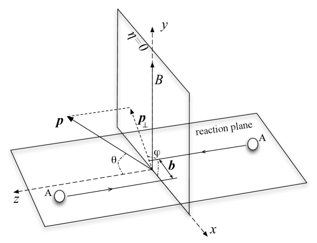
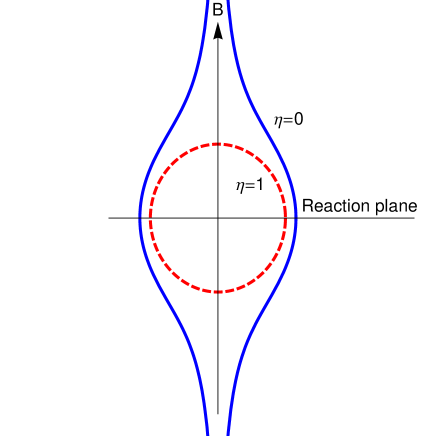
Throughout this article, the heavy-ion collision axis is denoted by . Average magnetic field then points in the -direction, see Fig. 1 and Fig. 7. Plane is the reaction plane and is the impact parameter.

§2 Magnetic field in vacuum
A Time-dependence
To obtain a quantitative estimate of magnetic field we need to take into account a realistic distribution of protons in a nucleus. This has been first done in Kharzeev:2007jp ***In the case of high-energy collisions, magnetic field was first estimated in Ambjorn:1990jg who also pointed out a possibility of formation of -condensate Ambjorn:1990jg ; Olesen:2012zb .. Magnetic field at point created by two heavy ions moving in the positive or negative -direction can be calculated using the Liénard-Wiechert potentials as follows
| (1.2) | ||||
| (1.3) |
with , where sums run over all protons in each nucleus, their positions and velocities being and . The magnitude of velocity is determined by the collision energy and the proton mass , . These formulas are derived in the eikonal approximation, assuming that protons travel on straight lines before and after the scattering. This is a good approximation since baryon stopping is a small effect at high energies. Positions of protons in heavy-ions can be determined by one of the standard models of the nuclear charge density . Ref.Kharzeev:2007jp employed the “hard sphere” model, while Bzdak:2011yy used a bit more realistic Wood-Saxon distribution.
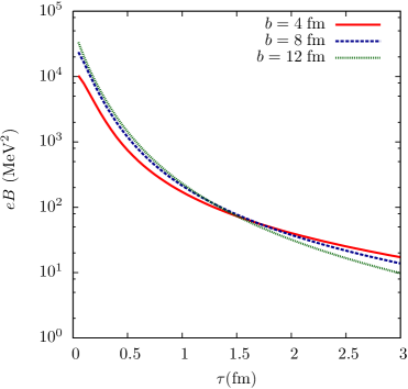
Numerical integration in (1.3) including small contribution from baryon stopping yields for magnetic field the result shown in Fig. 2 as a function of the proper time . Evidently, magnetic field rapidly decreases as a power of time, so that after first 3 fm it drops by more than three orders of magnitude.
 |
 |
B Event-by-event fluctuations in proton positions
Nuclear charge density provides only event-averaged distribution of protons. The actual distribution in a given event is different form implying that in a single event there is not only magnetic field along the -direction, but also other components of electric and magnetic fields. This leads to event-by-event fluctuations of electromagnetic field Bzdak:2011yy . Shown in Fig. 3 are electric and magnetic field components at at the origin (denoted by a black dot in Fig. 1) in collisions at GeV.
Fig. 3 clearly shows that although on average the only non-vanish component of the field is , which is also clear from the symmetry considerations, other components are finite in each event and are of the same order of magnitude
| (1.4) |
To appreciate the magnitude of electric field produced in heavy-ion collisions note that V/cm. The corresponding intensity is W/cm2 which is instructive to compare with the power generated by the most powerful state-of-the-art lasers: W/cm2.
 |
 |
Electromagnetic fields created in heavy-ion collisions were also examined in more elaborated approaches in Skokov:2009qp ; Voronyuk:2011jd ; Deng:2012pc . They yielded qualitatively similar results on electromagnetic field strength and its relaxation time.
§3 Magnetic field in quark-gluon plasma
A Liénard-Wiechert potentials in static medium
In the previous section I discussed electromagnetic field in vacuum. A more realistic estimate must include medium effects. Indeed, state-of-the art phenomenology of quark-gluon plasma (QGP) indicates that strongly interacting medium is formed at as early as 0.5 fm/c. Even before this time, strongly interacting medium exist in a form of Glasma Lappi:2006fp ; Blaizot:2012qd . Therefore, a calculation of magnetic field must involve response of medium determined by its electrical conductivity. It has been found in the lattice calculations that the gluon contribution to electrical conductivity of static quark-gluon plasma is Ding:2010ga
| (1.5) |
where is plasma temperature and its critical temperature. This agrees with Aarts:2007wj , but is at odds with an earlier calculation Gupta:2003zh . It is not clear whether (1.5) adequately describes the electromagnetic response of realistic quark-gluon plasma because it neglects quark contribution and assumes that medium is static. Theoretical calculations are of little help at the temperatures of interest since the perturbation theory is not applicable. In absence of a sensible alternative I will use (1.5) as a best estimate of electrical conductivity. If medium is static then is constant as a function of time . The static case is considered in this section, while in the next section I consider expanding medium.
In medium, magnetic field created by a charge moving in -direction with velocity is a solution of the following equations
| (1.6) | ||||
| (1.7) |
where we used the Ohm’s law to describe currents induced in the medium. Position of the observation point is specified by the longitudinal and transverse coordinates and , . Taking curl of the second equation in (1.7) and substituting eqs. (1.6) we get
| (1.8) |
The particular solution reads
| (1.9) |
where the Green’s function satisfies the following equation
| (1.10) |
which is solved by
| (1.11) |
where . Plugging this into (1.9) and substituting for the expression in the square brackets in (1.9) its Fourier image we obtain
| (1.12) | ||||
| (1.13) |
We are interested in the -component of the field. Noting that , where is the azimuthal angle in the transverse plane, and integrating over we derive
| (1.14) |
where we introduced notation
| (1.15) |
is the dielectric constant of the plasma with the following frequency dependence
| (1.16) |
Eq. (1.14) is actually valid for any functional form of Jackson's_text , which can be easily verified by using electric displacement instead of in eqs. (1.7). In this case (1.16) can be viewed as a low frequency expansion of . Magnetic field in this approximation is quasi-static. Therefore, we could have neglected the second time derivative in (1.8) and then keeping only the leading powers of we would have derived (1.14) with . After integration over this gives (1.21). Let us take notice of the fact that neglecting the second time derivative in (1.8) yields diffusion equation for magnetic field in plasma.
It is instructive to compare time-dependence of magnetic field created by moving charges in vacuum and in plasma. In vacuum, setting in (1.13) and integrating first over and then over gives
| (1.17) |
where we used . This coincides with (1.3) for a single proton when we take . Consider field strength (1.17) at the origin . At times the field is constant, while at it decreases as . At the time the ratio between these two is
| (1.18) |
which is a very small number ( at RHIC).
In matter . Let me write the modified Bessel function appearing in (1.14) as follows
| (1.19) |
Substituting (1.19) into (1.14) and using (1.16) we have ()
| (1.20) |
Closing the contour in the lower half-plane of complex picks a pole at . We have
| (1.21) |
At this function vanishes at and and has maximum at the time instant which is much larger than . The value of the magnetic field at this time is
| (1.22) |
(Here is the base of natural logarithm). This is smaller that the maximum field in vacuum
| (1.23) |
but is still a huge field. We compare the two solutions (1.17) and (1.21) in Fig. 4. We see that in a conducting medium magnetic field stays for a long time.
One essential component is still missing in our arguments – time-dependence of plasma properties due to its expansion. Let us now turn to this problem.

B Magnetic field in expanding medium
So far I treated quark-gluon plasma as a static medium. In expanding medium temperature and hence conductivity are functions of time. In Bjorken scenario Bjorken:1982qr , expansion is isentropic, i.e. , where is the particle number density and is plasma volume. Since and at early times expansion is one-dimensional it follows that . (Eventually, we will consider the midrapidity region , therefore distinction between the proper time and is not essential). Eq. (1.5) implies that . I will parameterize conductivity as follows
| (1.24) |
where I took fm to be the initial time (or longitudinal size) of plasma evolution. Suppose that plasma lives for 10 fm/c and then undergoes phase transition to hadronic gas at . Then employing (1.5) we estimate MeV. Let me define another parameter that I will need in the forthcoming calculation:
| (1.25) |
Magnetic field in expanding medium is still governed by (1.8). As was explained in the preceding subsection, time-evolution of magnetic field is quasi-static, which allows me to neglect the second time derivative. Let me introduce a new “time” variable as follows
| (1.26) |
Field satisfies equation
| (1.27) |
where
| (1.28) |
Its solution can be written as
| (1.29) |
in terms of the Green’s function satisfying
| (1.30) |
To solve this equation we represent as three-dimensional Fourier integral with respect to the space coordinates and Laplace transform with respect to the “time” coordinate:
| (1.31) |
with the contour C running parallel to the imaginary axis to the right of all integrand singularities. Now I would like to write the expression in the curly brackets in (1.29) also as Fourier-Laplace expansion. To this end we calculate
| (1.32) | ||||
| (1.33) |
Therefore,
| (1.34) |
Substituting (1.31) and (1.34) into (1.29) we obtain upon integration over the volume and time
| (1.35) |
where is the step-function. Taking consequent integrals over and gives
| (1.36) | ||||
| (1.37) |
Consider now . Integrating over azimuthal angle and then over as in (1.13),(1.14) yields
| (1.38) |
where .
The results of a numerical calculation of (1.38) are shown in Fig. 4. We see that expansion of plasma tends to increase the relaxation time, although this effect is rather modest. We conclude that due to finite electrical conductivity of QGP, magnetic field essentially freezes in the plasma for as long as plasma exists. Similar phenomenon, known as skin–effect, exists in good conductors placed in time-varying magnetic field: conductors expel time dependent magnetic fields form conductor volume confining them into a thin layer of width on the surface.
C Diffusion of magnetic field in QGP
The dynamics of magnetic field relaxation in conducting plasma plasma can be understood in a simple model Tuchin:2010vs . Suppose at some initial time magnetic field permits the plasma. The problem is to find the time-dependence of the field at . In this model, the field sources turn off at and do not at all contribute to the field at . Electromagnetic field is governed by the following equations
| (1.39) | |||||
| (1.40) |
that lead to the diffusion equation for , after we neglect the second time derivative as discussed before
| (1.41) |
For simplicity we treat electrical conductivity as constant. Initial condition at reads
| (1.42) |
where the Gaussian profile is chosen for illustration purposes and is the nuclear radius. Solution to the problem (1.41),(1.42) is
| (1.43) |
where the Green’s function is
| (1.44) |
Integrating over the entire volume we derive
| (1.45) |
It follows from (1.45) that as long as , where is a characteristic time magnetic field is approximately time-independent. This estimate is the same as the one we arrived at after (1.21).
In summary, magnetic field in quark-gluon plasma appears to be extremely strong and slowly varying function of time for most of the plasma life-time. At RHIC it decreases from right after the collision to at fm, see Fig. 4. This has a profound impact on all the processes occurring in QGP.
D Schwinger mechansim
Schwinger mechanism of pair production Schwinger:1951nm is operative if electric field exceeds the critical value of , where is mass of lightest electrically charged particle. Indeed, in order to excite a fermion out of the Dirac sea, electric force must do work along the path satisfying
| (1.46) |
If , then . The maximal value of is the fermion Compton’s wavelength implying that the minimum (or critical) value of electric field is
| (1.47) |
Notice that in stronger fields . Fig. 3 indicates that electron-positron pairs are certainly produced at RHIC. An important question then is the role of these pairs in the electromagnetic field relaxation in plasma. There are two associated effects: (i) before pairs thermalize, they contribute to the Foucault currents, (ii) after they thermalize, their density contributes to the polarization of plasma in electric field, and hence to its conductivity.
Since space dimensions of QGP are much less than fm, it may seem inevitable that space-dependence of electric field (in addition to its time-dependence) has a significant impact on the Schwinger process in heavy-ion collisions. However, his conclusion is premature. Indeed, suppose that electric field is a slow function of coordinates. Then . Work done by electric field is
| (1.48) |
where is length scale describing space variation of electric field. In order that contribution of space variation to work be negligible, the second term in the r.h.s. of (1.48) must satisfy . Employing the estimate that we obtained after (1.47) implies . Following Dunne:2005sx I define the inhomogeneity parameter
| (1.49) |
that describes the effect of spatial variation of electric field on the pair production rate. For electrons MeV in QGP fm at we have . Therefore, somewhat counter-intuitively , electric field can be considered as spatially homogeneous. The same conclusion can be derived from results of Wang:1988ct . Schwinger mechanism in spatially-dependent electric fields was also discussed in Martin:1988gr ; Kim:2007pm .
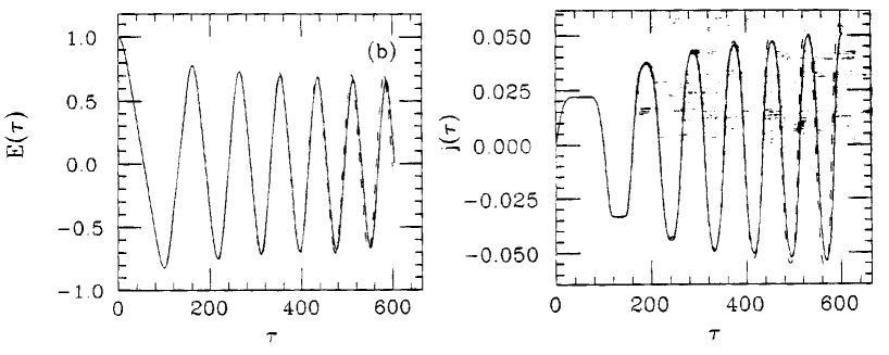
In view of smallness of one can employ the extensive literature on Schwinger effect in time-dependent spatially-homogeneous electric fields. As far as heavy-ion physics is concerned, the most comprehensive study has been done in Kluger:1992gb ; Cooper:1992hw ; Kluger:1991ib who developed an approach to include the effect of back reaction. They argued that time-evolution of electric field can be studied in adiabatic approximation and used the kinetic approach to study the time-evolution. Their results are exhibited in Fig. 5. Similar results were obtained in Tanji:2008ku . We observe that response time of the current density of Schwinger pairs fm/c is much larger than the plasma lifetime fm/c and therefore no sizable electric current is generated.
In summary, strong electric field is generated in heavy ion collisions in every event, but averages to zero in a large event ensemble. This field exceeds the critical value for electrons and light quarks. However, during the plasma lifetime no significant current of Schwinger pairs is generated.
2 Flow of quark-gluon plasma in strong magnetic field
§1 Azimuthal asymmetry
Magnetic field is known to have a profound influence on kinetic properties of plasmas. Once the spherical symmetry is broken, distribution of particles in plasma is only axially symmetric with respect to the magnetic field direction. This symmetry however is not manifest in the plane span by magnetic field and the impact parameter vectors, viz. -plane in Fig. 1. Charged particles moving along the magnetic field direction are not influenced by the magnetic Lorentz force while those moving the -plane (i.e. the reaction plane) are affected the most. The result is azimuthally anisotropic flow of expanding plasma in the -plane even when initial plasma geometry is completely spherically symmetric. The effect of weak magnetic field on quark-gluon plasma flow was first considered in Mohapatra:2011ku who argued that magnetic field is able to enhance the azimuthal anisotropy of produced particles up to . This conclusion was reached by utilizing a solution of the magneto-hydrodynamic equations in weak magnetic field.
A characteristic feature of the viscous pressure tensor in magnetic field is its azimuthal anisotropy. This anisotropy is the result of suppression of the momentum transfer in QGP in the direction perpendicular to the magnetic field. Its macroscopic manifestation is decrease of the viscous pressure tensor components in the plane perpendicular to the magnetic field, which coincides with the reaction plane in the heavy-ion phenomenology. Since Lorentz force vanishes in the direction parallel to the field, viscosity along that direction is not affected at all. In fact, the viscous pressure tensor component in the reaction plane is twice as small as the one in the field direction. As the result, transverse flow of QGP develops azimuthal anisotropy in presence of the magnetic field. Clearly, this anisotropy is completely different from the one generated by the anisotropic pressure gradients and exists even if the later are absent. In fact, because spherical symmetry in magnetic field is broken, viscous effects in plasma cannot be described by only two parameters: shear and bulk viscosity . Rather the viscous pressure tensor of magnetoactive plasma is characterized by seven viscosity coefficients, among which five are shear viscosities and two are bulk ones.
§2 Viscous pressure in strong magnetic field
A Viscosities from kinetic equation
Generally, calculation of the viscosities requires knowledge of the strong interaction dynamics of the QGP components. However, in strong magnetic field these interactions can be considered as a perturbation and viscosities can be analytically calculated using the kinetic equation LLX ; Erkelens:1977 . To apply this approach to QGP in strong magnetic field we start with kinetic equation for the distribution function of a quark flavor of charge is
| (2.1) |
where is the collision integral and is the electro-magnetic tensor, which contains only magnetic field components in the laboratory frame. Ellipsis in the argument of indicates the distribution functions of other quark flavors and gluons (I will omit them below). The equilibrium distribution reads
| (2.2) |
where is the macroscopic velocity of the fluid, is particle momentum, and is the mass density. Since , the first term on the r.h.s. of (2.1) as well as the collision integral vanishe in equilibrium. Therefore, we can write the kinetic equation as an equation for
| (2.3) |
where is a deviation from equilibrium. Differentiating (2.2) we find
| (2.4) |
Since and it follows that
| (2.5) |
Thus, in the comoving frame
| (2.6) |
Substituting (2.6) in (2.3) yields
| (2.7) |
where I defined
| (2.8) |
and used .
Since the time-derivative of is irrelevant for the calculation of the viscosity I will drop it from the kinetic equation. All indices thus become the usual three-vector ones. To avoid confusion we will label them by the Greek letters from the beginning of the alphabet. Introducing we cast (2.7) in the form
| (2.9) |
The viscous pressure generated by a deviation from equilibrium is given by the tensor
| (2.10) |
Effectively it can be parameterized in terms of the viscosity coefficients as follows (we neglect the bulk viscosities)
| (2.11) |
where the linearly independent tensors are given by
| (2.12a) | |||||
| (2.12b) | |||||
| (2.12c) | |||||
| (2.12d) | |||||
| (2.12e) | |||||
For the calculation of the shear viscosities , we can set and .
Let us expand to the second order in velocities in terms of the tensors as follows
| (2.13) |
Then, substituting (2.13) into (2.11) and requiring consistency of (2.10) and (2.11) yields
| (2.14) |
This gives the viscosities in the magnetic field in terms of the deviation of the distribution function from equilibrium. Transition to the non-relativistic limit in (2.14) is achieved by the replacement LLX .
B Collisionless plasma
In strong magnetic field we can determine by the method of consecutive approximations. Writing and substituting into (2.9) we find
| (2.15) |
Here I assumed that the deviation from equilibrium due to the strong magnetic field is much larger than due to the particle collisions. The explicit form of is determined by the strong interaction dynamics, but drops off the equation in the leading oder. The first correction to the equilibrium distribution obeys the equation
| (2.16) |
Using (2.13) we get
| (2.17) |
Substituting (2.17) into (2.16) and using (2.12) yields:
| (2.18) | |||||
where I used the following identities . Clearly, (2.18) is satisfied only if . Concerning the other two coefficients, we use the identities
| (2.19a) | |||||
| (2.19b) | |||||
that we substitute into (2.18) to derive
| (2.20) |
Since we obtain
| (2.21) |
Using (2.2), (2.21) in (2.14) in the comoving frame (of course ’s do not depend on the frame choice) and integrating using 3.547.9 of GR we derive Tuchin:2011jw
| (2.22) |
The non-relativistic limit corresponds to in which case we get
| (2.23) |
In the opposite ultra-relativistic case (high-temperature plasma)
| (2.24) |
where is the number density.
C Contribution of collisions
In the relaxation-time approximation we can write the collision integral as
| (2.25) |
where is an effective collision rate. Strong field limit means that
| (2.26) |
where is the synchrotron frequency. Whether itself is function of the field depends on the relation between the Larmor radius , where is the particle velocity in the plane orthogonal to and the Debye radius . If
| (2.27) |
then the effect of the field on the collision rate can be neglected LLX . Assuming that (2.27) is satisfied the collision rate reads
| (2.28) |
where is the transport cross section, which is a function of the saturation momentum Gribov:1984tu ; Blaizot:1987nc . We estimate , with GeV and with pressure GeV/fm3 we get MeV. Inequality (2.26) is well satisfied since Kharzeev:2007jp ; Skokov:2009qp and is in the range between the current and the constituent quark masses. On the other hand, applicability of the condition (2.27) is marginal and is very sensitive to the interaction details. In this section we assume that (2.27) holds in order to obtain the analytic solution. Additionally, the general condition for the applicability of the hydrodynamic approach , where is the mean free path and is the plasma size is assumed to hold. Altogether we have .
§3 Azimuthal asymmetry of transverse flow: a simple model
To illustrate the effect of the magnetic field on the viscous flow of the electrically charged component of the quark-gluon plasma I will assume that the flow is non-relativistic and use the Navie-Stokes equations that read
| (2.34) |
where is the viscous pressure tensor, is mass-density and is pressure. I will additionally assume that the flow is non-turbulent and that the plasma is non-compressible. The former assumption amounts to dropping the terms non-linear in velocity, while the later implies vanishing divergence of velocity
| (2.35) |
Because of the approximate boost invariance of the heavy-ion collisions, we can restrict our attention to the two dimensional flow in the plane corresponding to the central rapidity region.
The viscous pressure tensor in vanishing magnetic field is isotropic in the -plane and is given by
| (2.36) |
where the superscript indicates absence of the magnetic field. In the opposite case of very strong magnetic field the viscous pressure tensor has a different form (2.11). Neglecting all with we can write
| (2.37) |
where we also used (2.35). Notice that indicating that the plasma flows in the direction perpendicular to the magnetic field with twice as small viscosity as in the direction of the field. The later is not affected by the field at all, because the Lorentz force vanishes in the field direction. Substituting (2.37) into (2.34) we derive the following two equations characterizing the plasma velocity in the strong magnetic field Tuchin:2011jw
| (2.38) |
Additionally, we need to set the initial conditions
| (2.39) |
The solution to the the problem (2.38),(2.39) is
| (2.40a) | ||||
| (2.40b) | ||||
Here the Green’s function is given by
| (2.41) |
and the diffusion coefficient by
| (2.42) |
Suppose that the pressure is isotropic, i.e. it depends on the coordinates , only via the radial coordinate ; accordingly we pass from the integration variables and to in (2.40a) and (2.40b) correspondingly. At later times we can expand the Green’s function (2.41) in inverse powers of . The first terms in the r.h.s. of (2.40a) and (2.40b) are subleading and we obtain
| (2.43a) | ||||
| and by the same token | ||||
| (2.43b) | ||||
where denotes the boundary beyond which the density of the plasma is below the critical value. We observe that . Consequently, the azimuthal anisotropy of the hydrodynamic flow is Tuchin:2011jw
| (2.44) |
Since I assumed that the initial conditions and the pressure are isotropic, the azimuthal asymmetry (2.44) is generated exclusively by the magnetic field.
We see that at later times after the heavy-ion collision, flow velocity is proportional to , where is the finite shear viscosity coefficient, see (2.40a) and (2.40b). If the system is such that in absence of the magnetic field it were azimuthally symmetric, then the magnetic field induces azimuthal asymmetry of 1/3, see (2.44). The effect of the magnetic field on flow is strong and must be taken into account in phenomenological applications. Neglect of the contribution by the magnetic field leads to underestimation of the phenomenological value of viscosity extracted from the data Song:2007fn ; Romatschke:2007mq ; Dusling:2007gi . In other words, the more viscous QGP in magnetic field produces the same azimuthal anisotropy as a less viscous QGP in vacuum.
A model that I considered in this section to illustrate the effect of the magnetic field on the azimuthal anisotropy of a viscous fluid flow does not take into account many important features of a realistic heavy-ion collision. To be sure, a comprehensive approach must involve numerical solution of the relativistic magnetohydrodynamic equations with a realistic geometry. A potentially important effect that I have not considered here, is plasma instabilities Weibel ; Mrowczynski:1994xv , which warrant further investigation.
The structure of the viscous stress tensor in very strong magnetic field (2.37) is general, model independent. However, as explained, the precise amount of the azimuthal anisotropy that it generates cannot be determined without taking into account many important effects. Even so, I draw the reader’s attention to the fact that analysis of Mohapatra:2011ku using quite different arguments arrived at similar conclusion. Although a more quantitive numerical calculation is certainly required before a final conclusion can be made, it looks very plausible that the QGP viscosity is significantly higher than the presently accepted value extracted without taking into account the magnetic field effect Song:2007fn ; Romatschke:2007mq ; Dusling:2007gi and is perhaps closer to the value calculated using the perturbative theory Arnold:2003zc ; Baym:1990uj .
3 Energy loss and polarization due to synchrotron radiation
§1 Radiation of fast quark in magnetic field
General problem of charged fermion radiation in external magnetic field was solved in Nikishov:1964zza ; Sokolov:1963zn ; Ritus-dissertation . It has important applications in collider physics, see e.g. Berestetsky:1982aq ; Jackson:1975qi . In heavy-ion phenomenology, synchrotron radiation provides one of the mechanisms of energy loss in quark-gluon plasma, which is an important probe of QGP Gyulassy:1993hr ; Baier:1994bd .†††Synchrotron radiation in chromo-magnetic fields was discussed in Shuryak:2002ai ; Kharzeev:2008qr ; Zakharov:2008uk .
A typical diagram contributing to the synchrotron radiation, i.e. radiation in external magnetic field, by a quark is shown in Fig. 6 Tuchin:2010vs . This diagram is proportional to , where is the number of external field lines. In strong field, powers of must be summed up, which may be accomplished by exactly solving the Dirac equation for the relativistic fermion and then calculating the matrix element for the transition .

Such calculation has been done in QED for some special cases including the homogeneous constant field and can be readily generalized for gluon radiation. Intensity of the radiation can be expressed via the invariant parameter defined as
| (3.1) |
where the initial quark 4-momentum is , is the quark charge in units of the absolute value of the electron charge . At high energies,
| (3.2) |
The regime of weak fields corresponds to , while in strong fields . In our case, (at RHIC) and therefore . In terms of , spectrum of radiated gluons of frequency can be written as Nikishov:1964zza
| (3.3) |
where is the intensity,
and is the quark’s energy in the final state. is the Ayri function. Eq. (3.3) is valid under the assumption that the initial quark remains ultra-relativistic, which implies that the energy loss due to the synchrotron radiation should be small compared to the quark energy itself .
Energy loss by a relativistic quark per unit length is given by Berestetsky:1982aq
| (3.4) |
In two interesting limits, energy loss behaves quite differently. At we have Berestetsky:1982aq
| (3.5a) | |||||
| (3.5b) | |||||
In the strong field limit energy loss is independent of the quark mass, whereas in the weak field case it decreases as . Since , limit of corresponds to the classical energy loss.
To apply this result to heavy-ion collisions we need to write down the invariant in a suitable kinematic variables. The geometry of a heavy-ion collision is depicted in Fig. 7. Magnetic field is orthogonal to the reaction plane span by the impact parameter vector and the collision axis (-axis). For a quark of momentum we define the polar angle with respect to the -axis and azimuthal angle with respect to the reaction plane.
In this notation, and , where . Thus, . Conventionally, one expresses the longitudinal momentum and energy using the rapidity as and , where . We have
| (3.6) |
 |
|
 |
 |
In Fig. 8 a numerical calculation of the energy loss per unit length in a constant magnetic field using (3.4) and (3.6) is shown Tuchin:2010vs . We see that energy loss of a quark with GeV is about 0.2 GeV/fm at RHIC and 1.3 GeV/fm at LHC. This corresponds to the loss of 10% and 65% of its initial energy after traveling 5 fm at RHIC and LHC respectfully. Therefore, energy loss due to the synchrotron radiation at LHC gives a phenomenologically important contribution to the total energy loss.
Energy loss due to the synchrotron radiation has a very non-trivial azimuthal angle and rapidity dependence that comes from the corresponding dependence of the -parameter (3.6). As can be seen in Fig. 8(c), energy loss has a minimum at that corresponds to quark’s transverse momentum being parallel (or anti-parallel) to the field direction. It has a maximum at when is perpendicular to the field direction and thus lying in the reaction plane. It is obvious from (3.6) that at mid-rapidity the azimuthal angle dependence is much stronger pronounced than in the forward/backward direction. Let me emphasize, that the energy loss (3.4) divided by , i.e. scales with . In turn, is a function of magnetic field, quark mass, rapidity and azimuthal angle. Therefore, all the features seen in Fig. 8 follow from this scaling behavior.
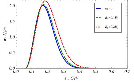
§2 Azimuthal asymmetry of gluon spectrum
In magnetic field gluon spectrum is azimuthally asymmetric. It is customary to describe this asymmetry by Fourier coefficients of intensity defined as
| (3.7) |
Azimuthal averaged intensity is . In strong fields and we can write
| (3.8) |
We have
| (3.9) |
At the Fourier coefficients can be calculated analytically using formula 3.631.9 of GR
| (3.10) |
where is the Euler’s Beta-function. The corresponding numerically values of the lowest harmonics are , , , , .
§3 Polarization of light quarks
Synchrotron radiation leads to polarization of electrically charged fermions; this is known as the Sokolov-Ternov effect Sokolov:1963zn . It was applied to heavy-ion collisions in Tuchin:2010vs . Unlike energy loss that I discussed so far, this is a purely quantum effect. It arises because the probability of the spin-flip transition depends on the orientation of the quark spin with respect to the direction of the magnetic field and on the sign of fermion’s electric charge. The spin-flip probability per unit time reads Sokolov:1963zn
| (3.11) |
where is a unit axial vector that coincides with the direction of quark spin in its rest frame, is the initial fermion velocity.
The nature of this spin-flip transition is transparent in the non-relativistic case, where it is induced by the interaction Hamiltonian Jackson:1975qi
| (3.12) |
It is seen, that negatively charged quarks and anti-quarks (e.g. and ) tend to align against the field, while the positively charged ones (e.g. and ) align parallel to the field.
Let be the number of fermions or anti-fermions with given momentum and spin direction parallel (anti-parallel) to the field produced in a given event. At initial time the spin-asymmetry defined as
| (3.13) |
vanishes. Eq. (3.11) implies that at later times, a beam of non-polarized fermions develops a finite asymmetry given by Sokolov:1963zn
| (3.14) |
where
| (3.15) |
is the characteristic time over which the maximal possible asymmetry is achieved. This time is extremely small on the scale of . For example, it takes only fm for a quark of momentum GeV at at RHIC to achieve the maximal asymmetry of %. Therefore, quarks and anti-quarks are polarized almost instantaneously after being released from their wave functions. However, subsequent interaction with QGP and fragmentation wash out the polarization of quarks.
A more sensitive probe are leptons weakly interacting with QGP and not undergoing a fragmentation process. Thus, their polarization can present a direct experimental evidence for the existence and strength of magnetic field. In case of muons we can estimate by replacing . For muons we get fm/c, which is still much smaller than magnetic field life-time. Observation of such a lepton polarization asymmetry is perhaps the most definitive proof of existence of the strong magnetic field at early times after a heavy-ion collision regardless of its later time-dependence.
In summary, energy loss per unit length for a light quark with GeV is about 0.27 GeV/fm at RHIC and 1.7 GeV/fm at LHC, which is comparable to the losses due to interaction with the plasma. Thus, the synchrotron radiation alone is able to account for quenching of jets at LHC with as large as 20 GeV. Synchrotron radiation is definetely one of missing pieces in the puzzle of the jet energy loss in heavy ion collisions. Quarks and leptons are expected to be strongly polarized in plasma in the direction parallel or anti-parallel to the magnetic field depending on the sign of their electric charge.
4 Photon decay
In this section I consider pair-production by photon in external magnetic field Tuchin:2010gx , which is a cross-channel of synchrotron radiation discussed in the previous section. Specifically, we are interested to determine photon decay rate in the process , where stands for a charged fermion, as a function of photon’s transverse momentum , rapidity and azimuthal angle . Origin of these photons in heavy-ion collisions will not be of interest to us in this section.
Characteristic frequency of a fermion of species of mass and charge ( is the absolute value of electron charge) moving in external magnetic field (in a plane perpendicular to the field direction) is
| (4.1) |
where is the fermion energy. Here – in the spirit of the adiabatic approximation – is a slow function of time. Calculation of the photon decay probability significantly simplifies if motion of electron is quasi-classical, i.e. quantization of fermion motion in the magnetic field can be neglected. This condition is fulfilled if . This implies that
| (4.2) |
For RHIC it is equivalent to , for LHC .
Photon decay rate was calculated in Nikishov:1964zza and, using the quasi-classical method, in Baier:1964 . It reads
| (4.3) |
where summation is over fermion species and the invariant parameter is defined as
| (4.4) |
with the initial photon 4-momentum . With notations of Fig. 7, , where . Thus, . Employing and we write
| (4.5) |
Plotted in Fig. 9 is the photon decay rate (4.3) for RHIC and LHC. The survival probability of photons in magnetic field is , where is the time spent by a photon in plasma. Estimating fm we determine that photon survives with probability % at RHIC, while only % at LHC. Such strong depletion can certainly be observed in heavy-ion collisions at LHC.
 |
 |
| (a) | (b) |
Azimuthal distribution of the decay rate of photons at LHC is azimuthally asymmetric as can be seen in Fig. 10 Tuchin:2010gx . The strongest suppression is in the field direction, i.e. in the direction orthogonal to the reaction plane. At the dependence of is very weak which is reflected in nearly symmetric azimuthal shape of the dashed line in Fig. 10.
To quantify the azimuthal asymmetry it is customary to expand the decay rate in Fourier series with respect to the azimuthal angle. Noting that is an even function of we have
| (4.6) |
In strong fields . For example, for at RHIC at and GeV we get . Therefore, we can expand the rate (4.3) at large as Nikishov:1964zza
| (4.7) |
At the Fourier coefficients can be calculated analytically using formula 3.631.9 of GR
| (4.8) |
where is the Euler’s Beta-function and is defined in (4.7). Substituting these expressions into (4.6) we find
| (4.9) |
The first few terms in this expansion read
| (4.10) |
What is measured experimentally is not the decay rate, but rather the photon spectrum. This spectrum is modified by the survival probability which is obviously azimuthally asymmetric. To quantify this asymmetry we write using (4.6)
| (4.11) |
where is the survival probability averaged over the azimuthal angle. Since , as can be seen in Fig. 9, we can estimate using (4.7) and (4.8)
| (4.12) |
In particular, the “elliptic flow” coefficient is Tuchin:2010gx
| (4.13) |
For example, at GeV and fm/c one expects % at RHIC and % at LHC only due to the presence of magnetic field. We see that decay of photons in external magnetic field significantly contributes to the photon asymmetry in heavy-ion collisions along with other possible effects.
In summary, I calculated photon pair-production rate in external magnetic field created in off-central heavy-ion collisions. Photon decay leads to depletion of the photon yield by a few percent at RHIC and by as much as 20% at the LHC. The decay rate depends on the rapidity and azimuthal angle. At mid-rapidity the azimuthal asymmetry of the decay rate translates into asymmetric photon yield and contributes to the “elliptic flow”. Let me also quote a known result that photons polarized parallel to the field are 3/2 times more likely to decay than those polarized transversely Nikishov:1964zza . Therefore, polarization of the final photon spectrum perpendicular to the field is a signature of existence of strong magnetic field. Finally, photon decay necessarily leads to enhancement of dilepton yield.
5 Quarkonium dissociation in magnetic field
§1 Effects of magnetic field on quarkonium
Strong magnetic field created in heavy-ion collisions generates a number of remarkable effects on quarkonium production some of which I will describe in this section. Magnetic field can be treated as static if the distance over which it significantly varies is much larger than the quarkonium radius. If is magnetic field life-time, then . For a quarkonium with binding energy and radius , the quasi-static approximation applies when . Estimating conservatively fm we get for : , which is comfortably large to justify the quasi-static approximation, where I assumed that is given by its vacuum value. As temperature increases drops. Temperature dependence of is model dependent, however it is certain that eventually it vanishes at some finite temperature . Therefore, only in the close vicinity of , i.e. at very small binding energies, the quasi-static approximation is not applicable. I thus rely on the quasi-static approximation to calculate dissociation Marasinghe:2011bt ; Tuchin:2011cg .
Magnetic field has a three-fold effect on quarkonium:
-
1.
Lorentz ionization. Consider quarkonium traveling with constant velocity in magnetic field in the laboratory frame. Boosting to the quarkonium comoving frame, we find mutually orthogonal electric and magnetic fields given by Eqs. (5.1),(5.2). In the presence of an electric field quark and antiquark have a finite probability to tunnel through the potential barrier thereby causing quarkonium dissociation. In atomic physics such a process is referred to as Lorentz ionization. In the non-relativistic approximation, the tunneling probability is of order unity when the electric field in the comoving frame satisfies (for weakly bound states), where is quark mass, see (5.24). This effect causes a significant increase in quarkonium dissociation rate; numerical calculation for is shown in Fig. 13.
-
2.
Zeeman effect. Energy of a quarkonium state depends on spin , orbital angular momentum , and total angular momentum . In a magnetic field these states split; the splitting energy in a weak field is , where is projection of the total angular momentum on the direction of magnetic field, is quark mass and is Landé factor depending on , and in a well-known way, see e.g. LL3-113 . For example, with , and () splits into three states with and with mass difference GeV, where we used . Thus, the Zeeman effect leads to the emergence of new quarkonium states in plasma.
-
3.
Distortion of the quarkonium potential in magnetic field. This effect arises in higher order perturbation theory and becomes important at field strengths of order Machet:2010yg . This is times stronger than the critical Schwinger’s field. Therefore, this effect can be neglected at the present collider energies.
Some of the notational definitions used in this section: and are velocity and momentum of quarkonium in the lab frame; is its mass; is the momentum of quark or anti-quark in the comoving frame; is its mass; is the magnetic field in the lab frame, and are electric and magnetic fields in the comoving frame; is the quarkonium Lorentz factor; and is a parameter defined in (5.19). I use Gauss units throughout the section; note that expressions , and are the same in Gauss and Lorentz-Heaviside units.
§2 Lorentz ionization: physical picture
In this section I focus on Lorentz ionization, which is an important mechanism of suppression in heavy-ion collisions Marasinghe:2011bt ; Tuchin:2011cg . Before we proceed to analytical calculations it is worthwhile to discuss the physics picture in more detail in two reference frames: the quarkonium proper frame and the lab frame. In the quarkonium proper frame the potential energy of, say, antiquark (with ) is a sum of its potential energy in the binding potential and its energy in the electric field , where is the electric field direction, see Fig. 11. Since becomes large and negative at large and negative (far away from the bound state) and because the quarkonium potential has finite radius, this region opens up for the motion of the antiquark. Thus there is a quantum mechanical probability to tunnel through the potential barrier formed on one side by the vanishing quarkonium potential and on the other by increasing absolute value of the antiquark energy in electric field. Of course the total energy of the antiquark (not counting its mass) is negative after tunneling. However, its kinetic energy grows proportionally to as it goes away. By picking up a light quark out of vacuum it can hadronize into a -meson.
If we now go to the reference frame where and there is only magnetic field (we can always do so since ), then the entire process looks quite different. An energetic quarkonium travels in external magnetic field and decays into quark-antiquark pair that can late hadronize into -mesons. This happens in spite of the fact that mass is smaller than masses of two -mesons due to additional momentum supplied by the magnetic field. Similarly a photon can decay into electron-positron pair in external magnetic field.
§3 Quarkonium ionization rate
A Comoving frame
Consider a quarkonium traveling with velocity in constant magnetic field . Let and be magnetic and electric fields in the comoving frame, and let subscripts and denote field components parallel and perpendicular to correspondingly. Then,
| (5.1a) | ||||
| (5.1b) | ||||
where . Clearly, in the comoving frame . If quarkonium travels at angle with respect to the magnetic field in the laboratory frame, then
| (5.2) |
We choose and axes of the comoving frame such that and . A convenient gauge choice is and . For a future reference we also define a useful dimensionless parameter Popov:1997-A
| (5.3) |
Note, that (i) because and (ii) when quarkonium moves perpendicularly to the magnetic field , .
B WKB method
I assume that the force binding and into quarkonium as a short-range one i.e. , where and are binding energy and mass of quarkonium, respectively, and is the radius of the nuclear force given by , where GeV/fm is the string tension. For example, the binding energy of and in in vacuum is GeV. This approximation is even better at finite temperature on account of decrease. Regarding as being bound by a short-range force enables us to calculate the dissociation probability with exponential accuracy , independently of the precise form of the quarkonium wave function. This is especially important since solutions of the relativistic two-body problem for quarkonium are not readily available.
It is natural to study quarkonium ionization in the comoving frame Marasinghe:2011bt . As explained in the Introduction, ionization is quantum tunneling through the potential barrier caused by the electric field . In this subsection I employ the quasi-classical WKB approximation to calculate the quarkonium decay probability . For the gauge choice specified in Sec. A quark energy () in electromagnetic field can be written as
| (5.4) |
In terms of , quarkonium binding energy is . To simplify notations, we will set , because the quark moves constant momentum along the direction of magnetic field.

We can see that the tunneling probability is finite only if . It is largest when . It has been already noted before in Popov:1998aw ; Popov:1997-A ; Popov:1998-A that the effect of the magnetic field is to stabilize the bound state. In spite of the linearly rising potential (at ) tunneling probability is finite as the result of rearrangement of the QED vacuum in electric field.
Ionization probability of quarkonium equals its tunneling probability through the potential barrier. The later is given by the transmission coefficient
| (5.5) |
In the non-relativistic approximation one can also calculate the pre-exponential factor, which appears due to the deviation of the quark wave function from the quasi-classical approximation. This is discussed later in Sec. B. We now proceed with the calculation of function . Since Eq. (5.4) can be written as Marasinghe:2011bt
| (5.6) |
where
| (5.7) |
Define dimensionless variables and . Integration in (2.27) gives:
| (5.8) |
For different ’s gives the corresponding ionization probabilities. The largest probability corresponds to smallest , which occurs at momentum determined by equation Popov:1998aw
| (5.9) |
Using (B) and parameter defined in (5.3) we find Marasinghe:2011bt
| (5.10) |
This is an implicit equation for the extremal momentum . Substituting into (B) one obtains , which by means of (5.5) yields the ionization probability. The quasi-classical approximation that we employed in this section is valid inasmuch as .
In order to compare with the results obtained in Popov:1998aw using the imaginary time method, we can re-write Eq. (5.10) in terms of an auxiliary parameter as
| (5.11a) | |||
| (5.11b) | |||
Taking advantage of these equations, Eq. (B) can be cast into a more compact form
| (5.12) |
where we denoted . This agrees with results of Ref. Popov:1998aw .
C Special case: Crossed fields
An important limiting case is crossed fields . Since also , see Sec. A, both field invariants vanish. Nevertheless, quarkonium ionization probability is finite Popov:1998aw . This limit is obtained by taking in the equations from the previous section. Employing (5.11a) and (5.11b) we get the following condition for extremum
| (5.13) |
with the solution
| (5.14) |
Substituting into (5.12) produces
| (5.15) |
§4 Non-relativistic approximation
A very useful approximation of the relativistic formulas derived in the previous section is the non-relativistic limit because (i) it provides a very good numerical estimate, see Fig. 12, (ii) it allows us to eliminate the parametric dependence in (B),(5.10) and write explicitly in terms of and , and (iii) spin effects can be accounted for Marasinghe:2011bt ; Tuchin:2011cg .
A Arbitrary binding
Motion of a particle can be treated non-relativistically if its momentum is much less than its mass. In such a case or . Additionally, motion of a charged particle in electromagnetic field is non-relativistic if . Indeed, the average velocity of a non-relativistic particle is of order . Thus, the non-relativistic limit is obtained by taking the limits and . In these limits the extremum conditions (5.11a),(5.11b) reduce to
| (5.16a) | |||
| (5.16b) | |||
Out of two solution to (5.16a) we pick the following one
| (5.17) |
The sign of is fixed using (5.16b) by noticing that . Eliminating gives:
| (5.18) |
where
| (5.19) |
is analogous to the adiabaticity parameter of Keldysh Keldysh-ioniz . Taking the non-relativistic limit of (5.12) and using (5.17) yields
| (5.20) |
where is the Keldysh function Keldysh-ioniz
| (5.21) |
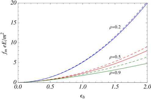
In Fig. 12 we show the dimensionless ratio as a function of the binding energy (in units of ) for several values of . The vacuum binding energy of corresponds to . We observe an excellent agreement between the full relativistic calculation and the non-relativistic approximation. At and the difference between the two lines is 10% and can be further improved by considering higher order corrections to Popov:1998-A .
B Weak binding
Of special interest is the limit of weak binding , i.e. . Expanding (5.18) at small and yields
| (5.22) |
and substituting into (5.21) and subsequently into (5.20) yields
| (5.23) |
Hence, the quarkonium dissociation probability reads LL3-77
| (5.24) |
Since the quasi-classical approximation employed in this paper is valid if , it follows that the binding energy must satisfy
| (5.25) |
Note also that we work in the approximation of the short-range binding potential meaning that , see Sec. §1.
C Strong binding
D Contribution of quark spin
So far I have neglected the contribution of quark spin. In order to take into account the effect of spin interaction with the external field, we can use squared Dirac equation for a bi-spinor :
| (5.30) |
where
| (5.35) |
Operators and do not commute. Therefore, in order to apply the WKB method for calculation of the ionization probability one actually needs to square (5.30), which leads to a differential equation of the fourth order in derivatives. The problem becomes more tractable in the non-relativistic case and for crossed fields. Spin effects in crossed fields were discussed in popov-review .
With quark spin taken into account, the non-relativistic version of (5.4) becomes:
| (5.36) |
and hence
| (5.37) |
where is the quark magnetic moment and is the projection of spin in the direction of the magnetic field. For a point quark, . The effect of quark spin on quarkonium dissociation probability can be taken into account by replacing in formulas for . With this replacement, all results of this section apply to a particle with spin. Note that effective binding energy decreases if spin is parallel to the magnetic field and increases if it is antiparallel. In particular, in the case of weak binding
| (5.38) |
Since the non-relativistic limit provide a good approximation of the full relativistic formulas, we will implement the quark spin dependence using the non-relativistic prescription Marasinghe:2011bt ; Tuchin:2011cg .
§5 Effect of electric field produced in the lab frame
A Origin of electric field in the lab frame
So far I have entirely neglected possible existence of electric field in the lab frame. This field, which we will denote by , can have two origins: (i) Asymmetry of nucleon distributions in the colliding heavy ions, see Fig. 3(b) and (ii) Chiral Magnetic Effect (CME) Kharzeev:2004ey ; Kharzeev:2007jp ; Kharzeev:2007tn ; Fukushima:2008xe ; Kharzeev:2009fn ; Basar:2010zd ; Asakawa:2010bu , which has recently attracted a lot of attention. In a nutshell, if a metastable and -odd bubble is induced by axial anomaly in the hot nuclear matter, then in the presence of external magnetic field the bubble generates an electric field which is parallel to the magnetic one. According to Kharzeev:2007tn the value of the electric field in the bubble is
| (5.39) |
where the sum runs over quark flavors and it is assumed that only three lightest flavors contribute. The value of the -angle fluctuates from event to event. CME refers to the macroscopic manifestation of this effect – separation of electric charges with respect to the reaction plane. This effect is a possible explanation of experimentally observed charge asymmetry fluctuations :2009uh ; :2009txa ; Ajitanand:2010rc .
No matter what is the origin of electric field in the lab frame, it averages to zero over an ensemble of events. We are interested to know the effect of this field on quarkonium dissociation – this is the problem we are turning to now Tuchin:2011cg .
B Quarkonium dissociation rate
Ionization probability of quarkonium equals its tunneling probability through the potential barrier. In the WKB approximation the later is given by the transmission coefficient and was calculated in Sec. §3. In this method contribution of the quark spin can be easily taken into account. Another method of calculating the ionization probability, the imaginary time method ITM1 ; ITM2 , was employed in Popov:1997-A ; Popov:1998-A ; Popov:1998aw . It also yielded in the non-relativistic approximation the pre-exponential factor that appears due to the deviation of the quark wave function from the quasi-classical approximation. Such a calculation requires matching quark wave function inside and outside the potential barrier LL3-77 . Extension of this approach to the relativistic case is challenging due to analytical difficulties of the relativistic two-body problem. Fortunately, it was argued in Sec. §3, that the non-relativistic approximation provides a very good accuracy in the region, which is relevant in the quarkiononium dissociation problem Popov:1998aw ; Marasinghe:2011bt .
Given the electromagnetic field in the laboratory frame , , the electromagnetic field , in the comoving frame moving with velocity is given by
| (5.40a) | ||||
| (5.40b) | ||||
where is a unit vector in the magnetic field direction, (see (5.39)) and . It follows from (5.40) that
| (5.41a) | ||||
| (5.41b) | ||||
Using (5.41) we find that the angle between the electric and magnetic field in the comoving frame is
| (5.42) |
where we used the relativistic invariance of .
It is useful to introduce dimensionless parameters , and as Popov:1998aw
| (5.43) |
where is quark mass and is quarkonium binding energy. I will treat the quarkonium binding potential in the non-relativistic approximation, which provides a very good accuracy to the dissociation rate Popov:1998aw ; Marasinghe:2011bt . The quarkonium dissociation rate in the comoving frame in the non-relativistic approximation is given by Popov:1997-A
| (5.44) |
where function reads
| (5.45) |
and functions and are given be the following formulas:
| (5.46) | ||||
| (5.47) | ||||
| (5.48) |
The contribution of quark spin is taken into account by replacing Marasinghe:2011bt . Function represents the leading quasi-classical exponent, is the pre-factor for the -wave state of quarkonium and accounts for the Coulomb interaction between the valence quarks. Parameter satisfies the following equation
| (5.49) |
which establishes its dependence on and . Note, that in the limit the dissociation rate (5.44) exponentially vanishes. This is because pure magnetic field cannot force a charge to tunnel through a potential barrier.
In the case that mechanism (i) is responsible for generation of electric field, is the field permitting the entire plasma in a single event. Event average is then obtained by averaging (5.44) over an ensemble of events. In the case that mechanism (ii) is operative, averaging is more complicated. Eq. (5.44) gives the quarkonium dissociation rate in a bubble with a given value of . Its derivation assumes that the dissociation process happens entirely inside a bubble and that is constant inside the bubble. Since in a relativistic heavy ion collision many bubbles can be produced with a certain distribution of ’s (with average ) more than one bubble can affect the dissociation process. This will result in a distractive interference leading to reduction of the -odd effect on quarkonium dissociation. However, if a typical bubble size is much larger than the size of quarkonium , then the dissociation is affected by one bubble at a time independently of others, and hence the interference effect can be neglected. In this case (2.27) provides, upon a proper average, a reasonable estimate of quarkonium dissociation in a heavy ion collision. We can estimate the bubble size as the size of the sphaleron, which is of the order of the chromo-magnetic screening length , whereas the quarkonium size is of the order . Consequently, at small coupling and below the zero-field dissociation temperature (i.e. when is not too small) is parametrically much larger than . A more quantitative estimate of the sphaleron size is fm Moore:2010jd ; whereas for fm. Thus, based on this estimate bubble interference can be neglected in the first approximation. However, since the ratio is actually not so small this effect nevertheless warrants further investigation.
To obtain the experimentally observed dissociation rate we need to average (2.27) over the bubbles produced in a given event and then over all events. To this end it is important to note that because the dissociation rate depends only on it is insensitive to the sign of the field or, in other words, it depends only on absolute value of but not on its sign. Therefore, it stands to reason that although the precise distribution of ’s is not known, (2.27) gives an approximate event average with parameter representing a characteristic absolute value of the theta-angle.
C Limiting cases
Before I proceed with the numerical calculations, let us consider for illustration several limiting cases. If quarkonium moves with non-relativistic velocity, then in the comoving frame electric and magnetic fields are approximately parallel , whereas in the ultra-relativistic case they are orthogonal , see (5.42). In the later case the electromagnetic field in the comoving frame does not depend on as seen in (5.41) and therefore the dissociation rate becomes insensitive to the CME. In our estimates I will assume that which is the relevant phenomenological situation. Indeed, it was proposed in Kharzeev:2007tn that produces charge fluctuations with respect to the reaction plane of the magnitude consistent with experimental data.
1) , i.e. electric and magnetic fields are approximately parallel. This situation is realized in the following two cases. (i) Non-relativistic quarkonium velocities: or (ii) motion of quarkonium at small angle to the direction of the magnetic field : . In both cases and . This is precisely the case where the dissociation rate exhibits its strongest sensitivity to the strength of the electric field generated by the local parity violating QCD effects. Depending on the value of the parameter defined in (5.43) we can distinguish the case of strong electric field and weak electric field Popov:1998-A . In the former case, , , . Substituting into (2.27) the dissociation rate reads
| (5.50) |
In the later case, and
| (5.51) |
where the electromagnetic field in the comoving frame equals one in the laboratory frame as was mentioned before.
2) , i.e. electric and magnetic fields are approximately orthogonal.‡‡‡Note, that the limit is different in and cases Popov:1997-A . This occurs for an ultra-relativistic motion of quarkonium . In this case
| (5.52) |
This case was discussed in detail in our previous paper Marasinghe:2011bt . In particular for we get
| (5.53) |
§6 Dissociation rate of
One of the most interesting applications of this formalism is calculation of the dissociation rate of which is considered a litmus test of the quark-gluon plasma Matsui:1986dk . Let be the heavy ions collision axis; heavy-ion collision geometry implies that . The plane containing -axis and perpendicular to the magnetic field direction is the reaction plane. We have
| (5.54) |
where is the angle between the directions of and and I denoted vector components in the -plane by the subscript . We can express the components of the quarkonium velocity in terms of the rapidity as , , where and are the quarkonium momentum and mass and .
 |
 |
| (a) | (b) |
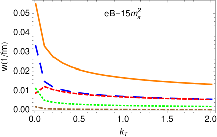
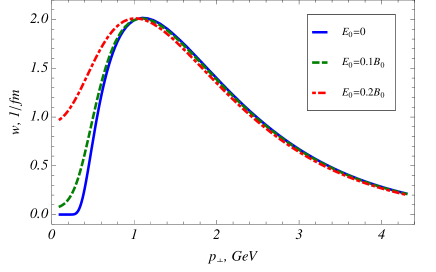
Results of numerical calculations are exhibited in Figs. 13–15 Tuchin:2011cg . In Fig. 13 I show the dissociation rate of for several values of the electric field induced by the Chiral Magnetic Effect. Note, that the typical size of the medium traversed by a quarkonium in magnetic field can be estimated very conservatively as a few fm. Therefore, fm-1 corresponds to complete destruction of ’s. This means that in the magnetic field of strength all ’s with GeV are destroyed independently of the strength of . Since magnetic field strength decreases towards the QGP periphery, most of surviving at later times originate from that region. Effect of electric field is strongest at low , which is consistent with our discussion in the previous section. The dissociation rate at low exponentially decreases with decrease of . Probability of quarkonium ionization by the fields below (i.e. ) is exponentially small. This is an order of magnitude higher than the estimate of electric field due to CME effect as proposed in Kharzeev:2007tn .

As the plasma temperature varies, so is the binding energy of quarkonium although the precise form of the function is model-dependent. The dissociation rate picks at some (see Fig. 13(b)), where is the binding energy in vacuum, indicating that breaks down even before drops to zero, which is the case at . This is a strong function of as can be seen in Fig. 14. It satisfies the equation . In the case (5.51) and (5.53) imply that
| (5.55) |
At and we employ (5.50) to derive the condition . In view of (5.52) and we obtain
| (5.56) |
where in the last step I used that . For a given function one can convert into the dissociation temperature, which is an important phenomenological parameter.
 |
 |
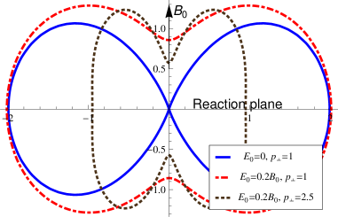
In the absence of electric fied , the dissociation probability peaks in the direction perpendicular to the direction of magnetic field , i.e. in the reaction plane. Dissociation rate vanishes in the direction. Indeed, for (5.41) implies that . This feature is seen in the left panel of Fig. 15. At finite the dissociation probability is finite in the direction making the azimuthal distribution more symmetric. The shape of the azimuthal distribution strongly depends on quarkonium velocity: while at low the strongest dissociation is in the direction of the reaction plane, at higher the maximum shifts towards small angles around the direction. Extrema of the azimuthal distribution are roots of the equation . At it yields minimum at , maximum at and another maximum that satisfies the condition (neglecting the spin-dependence of )
| (5.57) |
In order to satisfy (5.57) must decrease when increases and visa versa. This features are seen in the left panel of Fig. 15.
Spectrum of quarkonia surviving in the electromagnetic field is proportional to the survival probability , where is the time spent by the quarkonium in the field. Consider as a function of the angle between the quarkonium velocity and the reaction plane . Fourier expansion of in reads
| (5.58) |
Ellipticity of the distribution is characterized by the “elliptic flow” coefficient defined as
| (5.59) |
where denotes average of over the azimuthal angle. These formulas are applicable only as long as because otherwise there are no surviving quarkonia. In the right panel of Fig. 15 Tuchin:2011cg I show , which is independent of , as a function of . As expected, in the absence of the CME, is negative at low and positive at high . changes sign at that depends on the strength of the electric field. It decreases as increases until at it becomes positive at all . Fig. 15(b) provides the low bound for because and fm . We thus expect that magnetic field strongly modifies the azimuthal distribution of the produced ’s. Role of the magnetic field in generation of azimuthal anisotropies in heavy-ion collisions has been pointed out before in Tuchin:2010gx ; Mohapatra:2011ku .
In summary, we observed that dissociation energy increases with magnetic field strength and quarkonium momentum. As a consequence, quarkonia dissociate at lower temperature than one would have expected based on calculations neglecting magnetic field Marasinghe:2011bt ; Tuchin:2011cg . Fig. 13 indicates that in heavy-ion collisions at the LHC, all ’s moving with GeV in the reaction plane would dissociate with probability of order unity even if the QGP effect were completely negligible. If electric field fluctuations shown in Fig. 3 are taken into account, then even low ’s are destroyed. However, Chiral Magnetic Effect has negligible effect on dissociation.
Although magnetic fields in and collisions are much weaker than in collisions, they are still strong enough to cause dissociation at sufficiently high momenta . A truly spectacular feature of such process would be decay into two heavier -mesons.
The effect of dissociation in a magnetic field vanishes in the direction parallel to the magnetic field, i.e. perpendicular to the reaction plane. Therefore, dissociation gives negative contribution to the total azimuthal asymmetry coefficient . It remarkable that presence of electric field reverses this effect making positive.
6 Electromagnetic radiation by quark-gluon plasma in magnetic field
§1 Necessity to quantize fermion motion
In Sec. 3 we discussed synchrotron radiation of gluons by fast quarks. Our main interest was the energy loss problem. In this section we turn to the problem of electromagnetic radiation by QGP, viz. radiation of photons by thermal fermions Tuchin:2012mf . In this case quasi-classical approximation that we employed in Sec. 3 and Sec. 4 is no longer applicable and one has to take into account quantization of fermion motion in magnetic field.
Electromagnetic radiation by quarks and antiquarks of QGP moving in external magnetic field originates from two sources: (i) synchrotron radiation and (ii) quark and antiquark annihilation. QGP is transparent to the emitted electromagnetic radiation because its absorption coefficient is suppressed by . Thus, QGP is shinning in magnetic field. The main goal of this paper is to calculate the spectrum and angular distribution of this radiation. In strong magnetic field it is essential to account for quantization of fermion spectra. Indeed, spacing between the Landau levels is of the order ( being quark energy), while their thermal width is of the order . Spectrum quantization is negligible only if which is barely the case at RHIC and certainly not the case at LHC (at least during the first few fm’s of the evolution). Fermion spectrum quantization is important not only for hard and electromagnetic probes but also for the bulk properties of QGP.
§2 Synchrotron radiation
Motion of charged fermions in external magnetic field, which I will approximately treat as spatially homogeneous, is quasi-classical in the field direction and quantized in the reaction plane, which is perpendicular to the magnetic field and span by the impact parameter and the heavy ion collision axis. In high energy physics one usually distinguishes the transverse plane, which is perpendicular to the collision axis and span by the magnetic field and the impact parameter. In this section I use notation in which three-vectors are discriminated by the bold face and their component along the field direction by the plain face. Momentum projections onto the transverse plane are denoted by subscript .
In the configuration space, charged fermions move along spiral trajectories with the symmetry axis aligned with the field direction. Synchrotron radiation is a process of photon radiation by a fermion with electric charge in external magnetic field :
| (6.1) |
where is the photon momentum, are the momentum components along the magnetic field direction and indicies label the discrete Landau levels in the reaction plane. The Landau levels are given by
| (6.2) |
In the constant magnetic field only momentum component along the field direction is conserved. Thus, the conservation laws for synchrotron radiation read
| (6.3) |
where is the photon energy and is the photon emission angle with respect to the magnetic field. Intensity of the synchrotron radiation was derived in Sokolov:1968a . In Herold:1982a ; Harding:1987a ; Latal:1986a ; Baring:1988a it was thoroughly investigated as a possible mechanism for -ray bursts. In particular, synchrotron radiation in electromagnetic plasmas was calculated. Spectral intensity of angular distribution of synchrotron radiation by a fermion in the ’th Landau state is given by
| (6.4) |
where accounts for the double degeneration of all Landau levels except the ground one. The squares of matrix elements , which appear in (6.4), corresponding to photon polarization perpendicular and parallel to the magnetic field are given by, respectively,
| (6.5) | ||||
| (6.6) |
where for ,
| (6.7) |
and when . ( are identically zero). The functions are the generalized Laguerre polynomials. Their argument is
| (6.8) |
Angular distribution of radiation is obtained by integrating over the photon energies and remembering that also depends on by virtue of (6.2) and (6.3):
| (6.9) |
where photon energy is fixed to be
| (6.10) |
In the context of heavy-ion collisions the relevant observable is the differential photon spectrum. For ideal plasma in equilibrium each quark flavor gives the following contribution to the photon spectrum:
| (6.11) |
where accounts for quarks and antiquarks each of possible colors, and sums over the initial quark spin. Index indicates different quark flavors. stands for the plasma volume. The statistical factor is
| (6.12) |
The -function appearing in (6.4) can be re-written using (6.2) and (6.3) as
| (6.13) |
where
| (6.14) |
The following convenient notation was introduced:
| (6.15) |
The physical meaning of (§2) is that synchrotron radiation of a photon with energy at angle by a fermion undergoing transition from ’th to ’th Landau level is possible only if the initial quark momentum along the field direction equals .
Another consequence of the conservation laws (6.3) is that for a given and the photon energy cannot exceed a certain maximal value that will be denoted by . Indeed, inspection of (§2) reveals that this equation has a real solution only in two cases
| (6.16) |
The first case is relevant for the synchrotron radiation while the second one for the one-photon pair annihilation as discussed in the next section. Accordingly, allowed photon energies in the transition satisfy
| (6.17) |
No synchrotron radiation is possible for . In particular, when , , i.e. no photon is emitted, which is also evident in (6.10). The reason is clearly seen in the frame where : since , constraints (6.2) and (6.3) hold only if .
Substitution of (6.4) into (6.11) yields the spectral distribution of the synchrotron radiation rate per unit volume
| (6.18) |
where is the step-function.
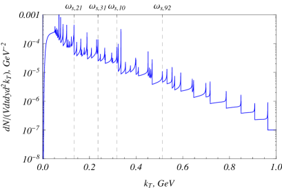
The natural variables to study the synchrotron radiation are the photon energy and its emission angle with respect to the magnetic field. However, in high energy physics particle spectra are traditionally presented in terms of rapidity (which for photons is equivalent to pseudo-rapidity) and transverse momentum . is a projection of three-momentum onto the transverse plane. These variables are not convenient to study electromagnetic processes in external magnetic field. In particular, they conceal the azimuthal symmetry with respect to the magnetic field direction. To change variables, let be the collision axis and be the direction of the magnetic field. In spherical coordinates photon momentum is given by , where and are the polar and azimuthal angles with respect to -axis. The plane is the reaction plane. By definition, implying that . Thus,
| (6.19) |
The second of these equations is the definition of (pseudo)-rapidity. Inverting (6.19) yields
| (6.20) |
Because the photon multiplicity in a unit volume per unit time reads
| (6.21) |
 |
 |
Fig. 16 displays the spectrum of synchrotron radiation by quarks as a function of at fixed Tuchin:2012mf . At midrapidity (6.20) implies that . Contribution of and quarks is qualitatively similar. At , quark masses do not affect the spectrum much. The main difference stems from the difference in electric charge. In panel (a) only the contributions of the first ten Landau levels are displayed. The cutoff frequencies can be clearly seen and some of them are indicated on the plot for convenience. The azimuthal distribution is shown in Fig. 17. Note, that at midrapidity . Therefore, the figure indicates that photon production in the direction of magnetic field (at ) is suppressed. More photons are produced in the direction of the reaction plane . This results in the ellipticity of the photon spectrum that translates into the positive “elliptic flow” coefficient . It should be noted, that the classical synchrotron radiation has a similar angular distribution.
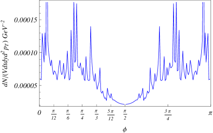
In order to compare the photon spectrum produced by synchrotron radiation to the photon spectrum measured in heavy-ion collisions, the , and quarks contributions were summed up. Furthermore, the experimental data from Adare:2008ab was divided by , where is the magnetic field relaxation time. The volume of the plasma can be estimated as with fm being the nuclear radius. Therefore,
| (6.22) |
The results are plotted in Fig. 18. In panel (a) it is seen that synchrotron radiation gives a significant contribution to the photon production in heavy-ion collisions at RHIC energy. This contribution is larger at small transverse momenta. This may explain enhancement of photon production observed in Adare:2008ab . Panel (b) indicates the increase of the photon spectrum produced by the synchrotron radiation mechanism at the LHC energy. This increase is due to enhancement of the magnetic field strength, but mostly because of increase of plasma temperature. This qualitative features can be better understood by considering the limiting cases of low and high photon energies.
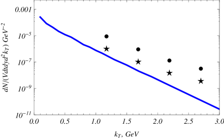 |
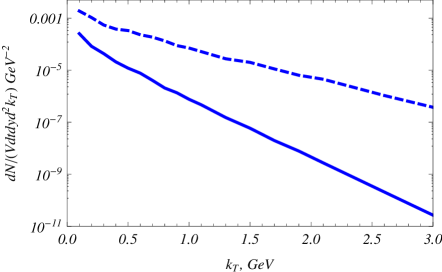 |
One possible way to ascertain the contribution of electromagnetic radiation in external magnetic field is to isolate the azimuthally symmetric component with respect to the direction of the magnetic field. It seems that synchrotron radiation dominates the photon spectrum at low . Thus, azimuthal symmetry can be easily checked by simply plotting the multiplicity vs , and , where is photon energy, is emission angle with respect to the magnetic field and is azimuthal angle around the magnetic field direction (which is perpendicular both to the collision axis and to the impact parameter). In Fig. 16(a) it is also seen that in these variables it may be possible to discern the cutoff frequencies that appear as resonances (in Fig. 16 so ). Note that averaging over the azimuthal angle around the collision axis direction destroys these features, see Fig. 18.
A Low photon energy
The low energy part of the photon spectrum satisfies the condition . The corresponding initial quark momentum component along the field and energy follow from (§2) and (6.2) and are given by
| (6.23) |
Evidently, . In practice, magnetic field strength satisfies , so that . Therefore, synchrotron radiation is dominated by fermion transitions from low Landau levels due to the statistical factors appearing in (6.11).
For a qualitative discussion it is sufficient to consider the transition. In this case the matrix elements (6.5) and (6.6) read
| (6.24) |
Assuming that the field strength is supercritical, i.e. , but keeping all powers of (for future reference) (§2) reduces to
| (6.25) |
Furthermore, using the conservation laws (6.3) we obtain in this approximation
| (6.26) | ||||
| (6.27) | ||||
| (6.28) |
The values of the non-vanishing matrix elements defined by (6.7) are
| (6.29) |
For , we write using (6.17) . Then (6.8) implies . Substituting (6.25)–(6.29) into (6.24) gives
| (6.30) |
According to (§2) the contribution of the transition to the synchrotron radiation reads Tuchin:2012mf
| (6.31) |
Consider radiation spectrum at , i.e. perpendicular to the magnetic field. The spectrum increases with and reaches maximum at . Since , spectrum decreases with increase of at fixed . This feature holds at low part of the spectrum for other emission angles and even for transitions form higher excited states. However, at high energies, it is no longer possible to approximate the spectrum by the contribution of a few low Landau levels. In that case the typical values of quantum numbers are . For example, to achieve the numerical accuracy of 5%, sum over must run up to a certain . Some values of are listed in Table 1 Tuchin:2012mf .
| 1 | 1 | 1 | 1 | 1 | 1 | 1 | 15 | 15 | 15 | |
| , GeV | 0.2 | 0.2 | 0.2 | 0.2 | 0.2 | 0.2 | 0.2 | 0.4 | 0.4 | 0.4 |
| , GeV | 0.1 | 1 | 2 | 3 | 1 | 1 | 1 | 1 | 2 | 1 |
| 0.096 | 9.6 | 38 | 86 | 29 | 35 | 19 | 0.64 | 2.6 | 1.3 | |
| 30 | 40 | 90 | 150 | 120 | 200 | 90 | 8 | 12 | 16 |
B High photon energy
The high energy tail of the photon spectrum is quasi-classical and approximately continuous. In this case the Laguerre polynomials can be approximated by the Airy functions or the corresponding modified Bessel functions. The angular distribution of the spectrum can be found in Baring:1988a :
| (6.32) |
provided that . Here is number density of flavor , which is independent of :
| (6.33) |
Here summation over was replaced by integration. It follows that this part of the spectrum increases with magnetic field strength as and and with temperature as . Therefore, variation of the spectrum with is much stronger than with . The dependence is shown in Fig. 19.
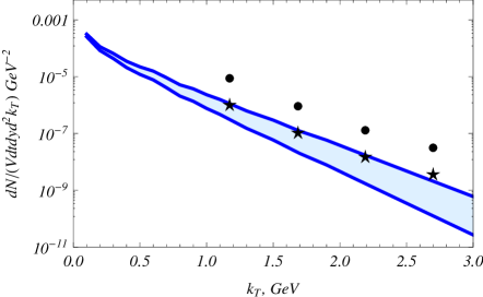
Unlike time-dependence of magnetic field, time-dependence of temperature is non-negligible even during the first few fm/c. Final synchrotron spectrum, which is an average over all temperatures, is dominated by high temperatures/early times. However, the precise form of time-dependence of temperature is model-dependent. Therefore, the spectrum is presented at fixed temperatures, so that a reader can appreciate its qualitative features in a model-independent way.
§3 Pair annihilation
The theory of one-photon pair annihilation was developed in Harding:1986a ; Wunner:1986a . It was shown in Wunner:1979a that in the super-critical regime one-photon annihilations is much larger than the two-photon annihilation. In this section the one-photon annihilation of and pairs in the QGP is calculated.
For pair annihilation the conservation of energy and momentum is given by
| (6.34) |
The spectral density of the annihilation rate per unit volume reads
| (6.35) |
where the matrix elements can be obtained from (6.5),(6.6) by making substitutions , and are given by
| (6.36) | ||||
| (6.37) |
with the same functions as in (6.7). Integration over removes the delta function responsible for the conservation of momentum along the field direction. The remaining delta function is responsible for energy conservation and can be written in exactly the same form as in (6.13) with particle energies and momenta now obeying the conservation laws (6.34). It is straightforward to see that momentum is still given by (§2),(6.15). The photon spectrum produced by annihilation of quark in state with antiquark in state has a threshold that is given by the case (ii) in (6.16):
| (6.38) |
Thus, the spectral density of the annihilation rate per unit volume is
| (6.39) |
Passing to and variables in place of and is similar to (6.21).
The results of the numerical calculations are represented in Fig. 20. Panel (a) shows the spectrum of photons radiated in annihilation of and . We conclude that contribution of the annihilation channel is negligible as compared to the synchrotron radiation.
 |
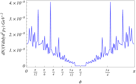 |
In summary, results of the calculations presented in this section indicate that photon production by QGP due to its interaction with external magnetic field give a considerable contribution to the total photon multiplicity in heavy-ion collisions. This is seen in Fig. 18 were the model calculation is compared with the experimental data Adare:2008ab . The largest contribution to the photon multiplicity arises from photon momenta of the order of . This may provide an explanation of the photon excess observed by the PHENIX experiment Adare:2008ab . Similar mechanism may also be responsible for enhancement of low mass di-lepton production that proceeds via emission of virtual photon which subsequently decays into di-lepton pair.
7 Summary
Analytical and numerical calculations indicate existence of extremely powerful electromagnetic fields in relativistic heavy ion collisions. They are the strongest electromagnetic fields that exist in nature. They evolve slowly on characteristic QGP time scale and therefore have a profound effect on dynamics of QGP. In this review I described the recent progress in understanding of particle production in presence of these fields. Treating the fields as quasi-static and spatially homogeneous allowed us to use analytical results derived over the past half-century. This is however the main source of uncertainty that can be clarified only in comprehensive numerical approach based on relativistic magnetohydrodynamics.
I discussed many spectacular effects caused by magnetic field. All of them have direct phenomenological relevance. Breaking of spherical symmetry by magnetic field in the direction perpendicular to the collision axis results in azimuthal asymmetry of particle production in the reaction plane. Fast quarks moving in magnetic field radiate a significant fraction of their energy. All electromagnetic probes are also naturally affected by magnetic field. Therefore, all experimental processes that are being used to study the properties of QGP have strong magnetic field dependence. In addition, the QCD phase diagram is modified by magnetic field as has been extensively studied using model calculations Gusynin:1995nb ; Chernodub:2010qx ; Hidaka:2012mz ; Chernodub:2012zx ; Mizher:2010zb ; Fraga:2008um ; Fraga:2012fs ; Gatto:2010pt ; Gatto:2010qs ; Osipov:2007je ; Kashiwa:2011js ; Johnson:2008vna ; Kanemura:1997vi ; Alexandre:2000yf ; Agasian:2008tb ; Preis:2010cq ; Miransky:2002rp ; Boomsma:2009yk ; Shushpanov:1997sf ; Cohen:2007bt ; Agasian:2001hv ; Galilo:2011nh and lattice simulations Cea:2005td ; Cea:2007yv ; Cea:2002wx ; Bali:2011qj ; Bali:2011uf ; Bali:2012zg ; Ilgenfritz:2012fw ; Aoki:2006we ; Nam:2011vn ; Bruckmann:2011zx ; D'Elia:2010nq ; D'Elia:2011zu ; Buividovich:2010tn . Entanglement of effects produced by magnetic field with conventional QGP ones makes it difficult to quantify the role of magnetic field in QGP dynamics. A unique observable is polarization of leptons escaping from QGP, which can be induced only by magnetic field, see Sec. §3.
Profound influence of magnetic field on properties of QGP is truly remarkable. Hopefully, progress in theory will soon be matched by experimental investigations that will eventually discover properties of QCD at high temperatures and strong electromagnetic fields.
Acknowledgements.
This work was supported in part by the U.S. Department of Energy under Grant No. DE-FG02-87ER40371.References
- (1) C. Kouveliotou, R. C. Duncan and C. Thompson, Sci. Am. 288N2, 24 (2003).
- (2) B. A. Boyko at. al., Pulsed Power Conference. Digest of Technical Papers. 12th IEEE International 2, 746 (1999).
- (3) J. S. Schwinger, Phys. Rev. 82, 664 (1951).
- (4) D. E. Kharzeev, L. D. McLerran and H. J. Warringa, Nucl. Phys. A 803, 227 (2008).
- (5) J. Ambjorn and P. Olesen, Phys. Lett. B 257, 201 (1991).
- (6) P. Olesen, arXiv:1207.7045 [hep-ph].
- (7) A. Bzdak and V. Skokov, Phys. Lett. B 710, 171 (2012).
- (8) V. Skokov, A. Y. Illarionov and V. Toneev, Int. J. Mod. Phys. A 24, 5925 (2009).
- (9) V. Voronyuk, V. D. Toneev, W. Cassing, E. L. Bratkovskaya, V. P. Konchakovski, S. A. Voloshin, Phys. Rev. C83, 054911 (2011).
- (10) W. -T. Deng and X. -G. Huang, Phys. Rev. C 85, 044907 (2012).
- (11) T. Lappi and L. McLerran, Nucl. Phys. A 772, 200 (2006) [hep-ph/0602189].
- (12) J. -P. Blaizot, F. Gelis, J. Liao, L. McLerran and R. Venugopalan, arXiv:1210.6838 [hep-ph].
- (13) J. D. Jackson, “Classical Electrodynamics”, 3rd edition.
- (14) H. T. Ding, A. Francis, O. Kaczmarek, F. Karsch, E. Laermann and W. Soeldner, arXiv:1012.4963 [hep-lat].
- (15) G. Aarts, C. Allton, J. Foley, S. Hands and S. Kim, Phys. Rev. Lett. 99, 022002 (2007) [arXiv:hep-lat/0703008].
- (16) S. Gupta, Phys. Lett. B 597, 57 (2004) [arXiv:hep-lat/0301006].
- (17) J. D. Bjorken, Phys. Rev. D 27, 140 (1983).
- (18) K. Tuchin, Phys. Rev. C 82, 034904 (2010) [Erratum-ibid. C 83, 039903 (2011)].
- (19) G. V. Dunne and C. Schubert, Phys. Rev. D 72, 105004 (2005) [hep-th/0507174].
- (20) R. -C. Wang and C. Y. Wong, Phys. Rev. D 38, 348 (1988).
- (21) C. Martin and D. Vautherin, Phys. Rev. D 40, 1667 (1989).
- (22) S. P. Kim and D. N. Page, Phys. Rev. D 75 (2007) 045013 [hep-th/0701047].
- (23) Y. Kluger, J. M. Eisenberg, B. Svetitsky, F. Cooper and E. Mottola, Phys. Rev. D 45, 4659 (1992).
- (24) F. Cooper, J. M. Eisenberg, Y. Kluger, E. Mottola and B. Svetitsky, Phys. Rev. D 48, 190 (1993) [hep-ph/9212206].
- (25) Y. Kluger, J. M. Eisenberg, B. Svetitsky, F. Cooper and E. Mottola, Phys. Rev. Lett. 67, 2427 (1991).
- (26) N. Tanji, Annals Phys. 324, 1691 (2009) [arXiv:0810.4429 [hep-ph]].
- (27) R. K. Mohapatra, P. S. Saumia and A. M. Srivastava, Mod. Phys. Lett. A 26, 2477 (2011).
- (28) E. M. Lifshitz, L. P. Pitaevskiy, “Physical kinetics”, Pergamon Press, 1981, §59.
- (29) H. Van Erkelens and W. A. Van Leeuwen, Physica A 89, 113-126 (1977); ibid. 89, 225-244 (1977), ibid. 90, 97-108 (1978).
- (30) K. Tuchin, J. Phys. G 39, 025010 (2012).
- (31) L. V. Gribov, E. M. Levin and M. G. Ryskin, Phys. Rept. 100, 1 (1983).
- (32) J. P. Blaizot and A. H. Mueller, Nucl. Phys. B 289, 847 (1987).
- (33) H. Song and U. W. Heinz, Phys. Lett. B 658, 279 (2008) [arXiv:0709.0742 [nucl-th]].
- (34) P. Romatschke and U. Romatschke, Phys. Rev. Lett. 99, 172301 (2007) [arXiv:0706.1522 [nucl-th]].
- (35) K. Dusling and D. Teaney, Phys. Rev. C 77, 034905 (2008) [arXiv:0710.5932 [nucl-th]].
- (36) P. Romatschke, Int. J. Mod. Phys. E19, 1-53 (2010). [arXiv:0902.3663 [hep-ph]].
- (37) E. S. Weibel, Phys. Rev. Lett. 2, 83 (1959).
- (38) S. Mrowczynski, Phys. Rev. C49, 2191-2197 (1994).
- (39) P. B. Arnold, G. D. Moore and L. G. Yaffe, JHEP 0305, 051 (2003) [arXiv:hep-ph/0302165].
- (40) G. Baym, H. Monien, C. J. Pethick and D. G. Ravenhall, Phys. Rev. Lett. 64, 1867 (1990).
- (41) A. I. Nikishov and V. I. Ritus, Sov. Phys. JETP 19, 529 (1964) [Zh. Eksp. Teor. Fiz. 46, 776 (1964)].
- (42) V. I. Ritus, J. Sov. Laser Res. 6, 497 (1985).
- (43) A. A. Sokolov and I. M. Ternov, Sov. Phys. Dokl. 8, 1203 (1964) [Dokl. Akad. Nauk Ser. Fiz. 153, 1052 (1964 PHDOE,8,1203-1205.1964)].
- (44) V. B. Berestetsky, E. M. Lifshitz and L. P. Pitaevsky, “Quantum Electrodynamics,” §90, Oxford, Uk: Pergamon (1982) 652 P. ( Course Of Theoretical Physics, 4)
- (45) J. D. Jackson, Rev. Mod. Phys. 48, 417 (1976).
- (46) M. Gyulassy and X. n. Wang, Nucl. Phys. B 420, 583 (1994) [arXiv:nucl-th/9306003].
- (47) R. Baier, Y. L. Dokshitzer, S. Peigne and D. Schiff, Phys. Lett. B 345, 277 (1995) [arXiv:hep-ph/9411409].
- (48) E. V. Shuryak and I. Zahed, Phys. Rev. D 67, 054025 (2003) [arXiv:hep-ph/0207163].
- (49) D. E. Kharzeev, arXiv:0806.0358 [hep-ph].
- (50) B. G. Zakharov, JETP Lett. 88, 475 (2008) [arXiv:0809.0599 [hep-ph]].
- (51) I.S. Gradshteyn, I.M. Ryzhik; Alan Jeffrey, Daniel Zwillinger, editors. Table of Integrals, Series, and Products, 7th edition. Academic Press, 2007.
- (52) K. Tuchin, Phys. Rev. C 83, 017901 (2011).
- (53) V. N. Baier and V. M. Katkov, Phys. Lett. A 25, 492 (1967).
- (54) T. Matsui and H. Satz, Phys. Lett. B 178, 416 (1986).
- (55) K. Marasinghe and K. Tuchin, Phys. Rev. C 84, 044908 (2011).
- (56) K. Tuchin, Phys. Lett. B 705, 482 (2011).
- (57) L. D. Landau and L. E. Lifshitz, “Quantum Mechanics Non-Relativistic Theory”, Butterworth-Heinemann, 3rd. ed., §113.
- (58) B. Machet and M. I. Vysotsky, Phys. Rev. D 83, 025022 (2011) [arXiv:1011.1762 [hep-ph]].
- (59) V. S. Popov, B. M. Karnakov and V. D. Mur, Phys. Lett. A 229, 306 (1997).
- (60) V. S. Popov, B. M. Karnakov and V. D. Mur, Phys. Lett. A 250, 20 (1998).
- (61) V. S. Popov, B. M. Karnakov and V. D. Mur, JETP 86, 860 (1998).
- (62) L. D. Landau and L. E. Lifshitz, “Quantum Mechanics Non-Relativistic Theory”, Butterworth-Heinemann, 3rd. ed., §77.
- (63) T.C. Scott, J. Shertzer, R.A. Moore, Phys. Rev. A 45, 4393 (1992).
- (64) L. V. Keldysh, Sov. Phys. JETP 20 1307 (1965).
- (65) V. S. Popov. Physics Uspekhi, 47, 855 (2004).
- (66) D. Kharzeev, Phys. Lett. B633, 260-264 (2006).
- (67) D. Kharzeev and A. Zhitnitsky, Nucl. Phys. A 797, 67 (2007) [arXiv:0706.1026 [hep-ph]].
- (68) K. Fukushima, D. E. Kharzeev and H. J. Warringa, Phys. Rev. D 78, 074033 (2008) [arXiv:0808.3382 [hep-ph]].
- (69) D. E. Kharzeev, Annals Phys. 325, 205-218 (2010). [arXiv:0911.3715 [hep-ph]].
- (70) G. Basar, G. V. Dunne and D. E. Kharzeev, arXiv:1003.3464 [hep-ph].
- (71) M. Asakawa, A. Majumder and B. Muller, arXiv:1003.2436 [hep-ph].
- (72) B. I. Abelev et al. [STAR Collaboration], Phys. Rev. Lett. 103, 251601 (2009) [arXiv:0909.1739 [nucl-ex]].
- (73) B. I. Abelev et al. [STAR Collaboration], Phys. Rev. C 81, 054908 (2010) [arXiv:0909.1717 [nucl-ex]].
- (74) N. N. Ajitanand, R. A. Lacey, A. Taranenko and J. M. Alexander, Phys. Rev. C 83 (2011) 011901 [arXiv:1009.5624 [nucl-ex]].
- (75) A.M. Perelomov, V.S. Popov and M.V. Terent ev, Zh. Eksp. Tear. Fiz. 50 (1966) 1393; 51 (1966) 309.
- (76) V.S. Popov, V.P. Kuznetzov and A.M. Perelomov, Zh. Eksp. Teor. Fiz. 53 (1967) 331.
- (77) G. D. Moore and M. Tassler, JHEP 1102, 105 (2011) [arXiv:1011.1167 [hep-ph]].
- (78) K. Tuchin, arXiv:1206.0485 [hep-ph].
- (79) A. A. Sokolov and I. M. Ternov, “Synchrotron radiation”, Pergamon Press, Oxford, (1968).
- (80) M. G. Baring, Mon. Not. R. ast. Soc. 235, 57, (1988).
- (81) H. Herold, H. Ruder and G. Wunner, Astron. Astrophys. 115, 90, (1982).
- (82) A. K. Harding and R. Preece, Ap. J. 319, 939, (1987).
- (83) H. G. Latal, Ap. J. 309, 372, (1986).
- (84) A. Adare et al. [PHENIX Collaboration], Phys. Rev. Lett. 104, 132301 (2010).
- (85) A. K. Harding, Ap. J. 300, 167, (1986).
- (86) G. Wunner, J. Paez, H. Herold and H. Ruder, Astron. Astrophys. 170, 179, (1986)
- (87) G. Wunner, Phys. Rev. Lett. 42, 79, (1979).
- (88) A. J. Mizher, M. N. Chernodub and E. S. Fraga, Phys. Rev. D 82, 105016 (2010)
- (89) E. S. Fraga and A. J. Mizher, Nucl. Phys. A 820, 103C (2009)
- (90) E. S. Fraga and L. F. Palhares, Phys. Rev. D 86, 016008 (2012).
- (91) R. Gatto and M. Ruggieri, Phys. Rev. D 83, 034016 (2011).
- (92) R. Gatto and M. Ruggieri, Phys. Rev. D 82, 054027 (2010).
- (93) A. A. Osipov, B. Hiller, A. H. Blin and J. da Providencia, Phys. Lett. B 650, 262 (2007).
- (94) K. Kashiwa, Phys. Rev. D 83, 117901 (2011).
- (95) C. V. Johnson and A. Kundu, JHEP 0812, 053 (2008).
- (96) S. Kanemura, H. -T. Sato and H. Tochimura, Nucl. Phys. B 517, 567 (1998).
- (97) J. Alexandre, K. Farakos and G. Koutsoumbas, Phys. Rev. D 63, 065015 (2001).
- (98) N. O. Agasian and S. M. Fedorov, Phys. Lett. B 663, 445 (2008).
- (99) F. Preis, A. Rebhan and A. Schmitt, JHEP 1103, 033 (2011).
- (100) V. P. Gusynin, V. A. Miransky and I. A. Shovkovy, Nucl. Phys. B 462, 249 (1996).
- (101) V. A. Miransky and I. A. Shovkovy, Phys. Rev. D 66, 045006 (2002).
- (102) M. N. Chernodub, Phys. Rev. D 82, 085011 (2010) [arXiv:1008.1055 [hep-ph]].
- (103) Y. Hidaka and A. Yamamoto, arXiv:1209.0007 [hep-ph].
- (104) M. N. Chernodub, Phys. Rev. D 86, 107703 (2012) [arXiv:1209.3587 [hep-ph]].
- (105) J. K. Boomsma and D. Boer, Phys. Rev. D 81, 074005 (2010).
- (106) I. A. Shushpanov and A. V. Smilga, Phys. Lett. B 402, 351 (1997).
- (107) T. D. Cohen, D. A. McGady and E. S. Werbos, Phys. Rev. C 76, 055201 (2007).
- (108) N. O. Agasian, Phys. Atom. Nucl. 64, 554 (2001) [Yad. Fiz. 64, 608 (2001)].
- (109) B. V. Galilo and S. N. Nedelko, Phys. Rev. D 84, 094017 (2011) [arXiv:1107.4737 [hep-ph]].
- (110) M. D’Elia, S. Mukherjee and F. Sanfilippo, Phys. Rev. D 82, 051501 (2010).
- (111) P. Cea and L. Cosmai, JHEP 0508, 079 (2005).
- (112) P. Cea and L. Cosmai, JHEP 0302, 031 (2003).
- (113) P. Cea, L. Cosmai and M. D’Elia, JHEP 0712, 097 (2007).
- (114) G. S. Bali et. al., JHEP 1202, 044 (2012).
- (115) G. S. Bali, F. Bruckmann, G. Endrodi, Z. Fodor, S. D. Katz, S. Krieg, A. Schafer and K. K. Szabo, PoS LATTICE 2011, 192 (2011) [arXiv:1111.5155 [hep-lat]].
- (116) G. S. Bali, F. Bruckmann, G. Endrodi, Z. Fodor, S. D. Katz and A. Schafer, Phys. Rev. D 86, 071502 (2012) [arXiv:1206.4205 [hep-lat]].
- (117) E. -M. Ilgenfritz, M. Kalinowski, M. Muller-Preussker, B. Petersson and A. Schreiber, Phys. Rev. D 85, 114504 (2012) [arXiv:1203.3360 [hep-lat]].
- (118) Y. Aoki, G. Endrodi, Z. Fodor, S. D. Katz and K. K. Szabo, Nature 443, 675 (2006) [hep-lat/0611014].
- (119) S. -i. Nam and C. -W. Kao, Phys. Rev. D 83, 096009 (2011) [arXiv:1103.6057 [hep-ph]].
- (120) M. D’Elia and F. Negro, Phys. Rev. D 83, 114028 (2011) [arXiv:1103.2080 [hep-lat]].
- (121) P. V. Buividovich, M. N. Chernodub, D. E. Kharzeev, T. Kalaydzhyan, E. V. Luschevskaya and M. I. Polikarpov, arXiv:1003.2180 [hep-lat].
- (122) F. Bruckmann and G. Endrodi, Phys. Rev. D 84, 074506 (2011) [arXiv:1104.5664 [hep-lat]].