Opportunistic DF-AF Selection Relaying with Optimal Relay Selection in Nakagami-$m$ Fading Environments

Abstract

An opportunistic DF-AF selection relaying scheme with maximal received signal-to-noise ratio (SNR) at the destination is investigated in this paper. The outage probability of the opportunistic DF-AF selection relaying scheme over Nakagami-$m$ fading channels is analyzed, and a closed-form solution is obtained. We perform asymptotic analysis of the outage probability in high SNR domain. The coding gain and the diversity order are obtained. For the purpose of comparison, the asymptotic analysis of opportunistic AF scheme in Nakagami-$m$ fading channels is also performed by using the Squeeze Theorem. In addition, we prove that compared with the opportunistic DF scheme and opportunistic AF scheme, the opportunistic DF-AF selection relaying scheme has better outage performance.

I Introduction

Coperative diversity, which lets the single antenna equipped communication terminal enjoy the performance gain from spatial diversity, is an important modus operandi of substantially improving coverage and performance in wireless networks. The basic idea is that beside the direct transmission from the source to the destination, some adjacent nodes can be used to obtain the diversity by relaying the source signal to the destination [1, 2]. Several cooperative diversity protocols including amplify-and-forward (AF), decode-and-forward (DF), selection relaying and incremental relaying, have been discussed in [2]-[4]. DF-AF selection relaying protocol, where each relay can adaptively switch between DF and AF according to its local signal-to-noise ratio (SNR), has been developed and investigated in [5]-[8].

For the purpose of improving the system spectral efficiency, the opportunistic relaying scheme for cooperative networks has been introduced [9, 10]. In such a scheme, a single relay is selected from a set of relay nodes. The opportunistic DF protocol and opportunistic AF protocol have been well studied in Rayleigh fading channels [11]-[15]. In contrast, the opportunistic relaying over Nakagami-$m$ fading channels have not been extensively studied yet due to the mathematical difficulty. Furthermore, when each relay utilizes DF-AF selection relaying protocol, how to choose a best one among them?

In this paper, we study the opportunistic DF-AF selection relaying with optimal relay selection whereby the destination obtains maximal received SNR in cooperative networks. Moreover, we carry out asymptotic outage behavior analysis of the opportunistic DF-AF selection relaying scheme in Nakagami-$m$ fading channels. In addition, the asymptotic performance of opportunistic AF protocol in Nakagami-$m$ fading channels is analyzed for comparison.

The rest of the paper is structured as follows. Section II introduces the opportunistic DF-AF selection relaying scheme. Section III presents the asymptotic outage analysis of the opportunistic DF-AF selection relaying. Next, in Section IV, comparisons with the opportunistic DF scheme and opportunistic AF scheme are performed. In Section V, the numerical results are presented. Finally, the main results of the paper are summarized in Section VI.

II Description of opportunistic DF-AF selection relaying

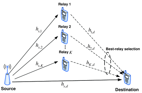
Figure 1: Wireless relay channel

Consider a cooperative wireless network consisting of a source node ($S$), a destination node ($D$) and $K$ potential relays $\mathbb{R}=(R_{1},R_{2},\ldots,R_{K})$ as shown in Fig. 1. Instantaneous SNRs of $S\rightarrow D$, $S\rightarrow R_{i}$ and $R_{i}\rightarrow D$ channels are denoted by $\gamma_{0}$, $\gamma_{1i}$ and $\gamma_{2i}$, where $i=1,2,\cdots,K$. The effects of the fading are captured by complex channel gains $h_{s,d}$, $h_{s,i}$ and $h_{i,d}$ respectively. The fading in each channel is assumed to be independent, slow and Nakagami-$m$ distributed with parameters $(m_{0},\omega_{0})$, $(m_{1i},\omega_{1i})$, and $(m_{2i},\omega_{2i})$ respectively. We have $\gamma_{0}=|h_{s,d}|^{2}\mathsf{SNR}$, $\gamma_{1i}=|h_{s,i}|^{2}\mathsf{SNR}$, and $\gamma_{2i}=|h_{i,d}|^{2}\mathsf{SNR}$, where $\mathsf{SNR}$ is the transmit SNR.

In opportunistic DF-AF selection relaying, among the $K$-relay set, where each relay uses DF-AF selection relaying protocol, a “best” relay will be selected for each transmission. Such a cooperative transmission is divided into two steps with equal durations. In the first step the source node broadcasts its signal to the destination node and the set of $K$-relay nodes as well. In the second step, the best relay $R_{b}$ is selected according to

$$b=\arg\max_{i=1,2,\cdots,K}\left\{\xi_{i}\gamma_{2i}+(1-\xi_{i})\frac{\gamma_{1i}\gamma_{2i}}{\gamma_{1i}+\gamma_{2i}+1}\right\},$$ (1)

where $\xi_{i}$ denotes the decoding state of $R_{i}$, i.e., $\xi_{i}=1$ when $R_{i}$ could fully decode the source message, otherwise $\xi_{i}=0$. And the best relay $R_{b}$ will use DF-AF selection relaying protocol to forward the received signal. Specifically, relay $R_{b}$ uses DF to re-transmit the received signal if $\xi_{b}=1$. Otherwise AF will be used. Since combing method does not affect the diversity order analysis, we assume that the destination uses Selection Combining (SC) to combine the signals received in the two stages for tractability unless otherwise specified.

Remark: Let path $0$ represent the direct link ($S\rightarrow D$) and path $i$ represent the $i^{th}$ cascaded link ($S\rightarrow R_{i}\rightarrow D$) where $i=1,\cdots,K$. For the $i^{th}$ cascaded link we introduce a random variable $\gamma_{i}$ that will denote the equivalent instantaneous SNR at the destination [15]. That is, let $\gamma_{i}$ takes into account both the fading on $S\rightarrow R_{i}$ link and the fading on the $R_{i}\rightarrow D$ link. $\gamma_{i}=\gamma_{2i}$ when $R_{i}$ uses DF, otherwise if AF is used by $R_{i}$, $\gamma_{i}=\frac{\gamma_{1i}\gamma_{2i}}{\gamma_{1i}+\gamma_{2i}+1}$ [2]. Then we have

$$\gamma_{i}=\xi_{i}\gamma_{2i}+(1-\xi_{i})\frac{\gamma_{1i}\gamma_{2i}}{\gamma_{1i}+\gamma_{2i}+1}.$$ (2)

Combining (1) and (2), it can be shown that the proposed selection method of the best relay gives the maximal equivalent instantaneous SNR of $S\rightarrow R_{b}\rightarrow D$ path. On the other hand, as Selection Combining (SC) is used at the destination. The received SNR at the destination can be given by $\gamma=\max\{\gamma_{0},\gamma_{b}\}.$ Hence the proposed selection method of the best relay gives the maximal received SNR at the destination.

III Outage analysis of the opportunistic DF-AF selection relaying scheme

The outage probability can be given by the following lemma.

Lemma 1.

The outage probability of the opportunistic DF-AF selection relaying scheme can be given by

$$P_{out}=\bigg{[}1-\frac{\Gamma\left(m_{0},\alpha_{0}\gamma_{th}\right)}{\Gamma\left(m_{0}\right)}\bigg{]}\prod_{i=1}^{K}\Bigg{[}\frac{\Gamma\left(m_{1i},\alpha_{1i}\Delta\right)}{\Gamma\left(m_{1i}\right)}\Bigg{(}1$$ (3)

$$- \frac{\Gamma\left(m_{2i},\alpha_{2i}\gamma_{th}\right)}{\Gamma\left(m_{2i}\right)}\Bigg{)}+\Bigg{(}1-\frac{\Gamma\left(m_{1i},\alpha_{1i}\Delta\right)}{\Gamma\left(m_{1i}\right)}\Bigg{)}\Bigg{]},$$

where $R$ is the transmission rate, $\Delta=2^{2R}-1$ and $\gamma_{th}$ is the SNR threshold at the destination. $\alpha_{0}=\frac{m_{0}}{\overline{\gamma}_{0}}$, $\alpha_{1i}=\frac{m_{1i}}{\overline{\gamma}_{1i}}$, and $\alpha_{2i}=\frac{m_{2i}}{\overline{\gamma}_{2i}}$, $\Gamma(\cdot)$ is the gamma function, and $\Gamma(\cdot,\cdot)$ is the incomplete gamma function.

Proof:

Throughout this paper, we use $X\sim\mathcal{G}(m)$ to denote that a random variable $X$ has the p.d.f. given by $f_{X}(y)=\frac{1}{\Gamma(m)}\left(\frac{m}{\overline{X}}\right)^{m}y^{m-1}e^{-\frac{my}{\overline{X}}}.$ First, it can be derived that c.d.f. of $Y\sim\mathcal{G}(m)$ can be given by

$$F_{Y}(y)=1-\frac{\Gamma\left(m,\frac{my}{\overline{Y}}\right)}{\Gamma\left(m\right)}.$$ (4)

If the source-relay link is able to support $R$, i.e., $\frac{1}{2}\log_{2}\left(1+\gamma_{1i}\right)\geq R,$ or equivalently, if $\gamma_{1i}\geq\Delta=2^{2R}-1,$ the relay could fully decode the source message. Consequently, the instantaneous equivalent end-to-end SNR per symbol at the destination is $\gamma=\max\left(\gamma_{0},\max_{i=1,2,\cdots,K}\left\{\xi_{i}\gamma_{2i}+(1-\xi_{i})\frac{\gamma_{1i}\gamma_{2i}}{\gamma_{1i}+\gamma_{2i}+1}\right\}\right),$ where $\Pr\{\xi_{i}=0\}=\Pr\{\gamma_{1i}<\Delta\}=F_{\gamma_{1i}}(\Delta)$ and $\Pr\{\xi_{i}=1\}=1-\Pr\{\xi_{i}=0\}.$ The outage probability can be given by $P_{out}=\Pr\left\{\gamma<\gamma_{th}\right\}=\Pr\left\{\gamma_{0}<\gamma_{th}\right\}\prod_{i=1}^{K}\Pr\left\{\xi_{i}\gamma_{2i}+(1-\xi_{i})\frac{\gamma_{1i}\gamma_{2i}}{\gamma_{1i}+\gamma_{2i}+1}<\gamma_{th}\right\}.$ According to the Theorem of Total Probability and conditional probability, we have

$$P_{out} = \Pr\{\gamma_{0}<\gamma_{th}\}\prod_{i=1}^{K}\Big{(}\Pr\{\xi_{i}=1\}\Pr\{\gamma_{2i}<\gamma_{th}\}$$ (5)

$$+ \Pr\{\xi_{i}=0\}\Pr\Big{\{}\frac{\gamma_{1i}\gamma_{2i}}{\gamma_{1i}+\gamma_{2i}+1}<\gamma_{th}|\xi_{i}=0\Big{\}}\Big{)}$$

$$\stackrel{{\scriptstyle(a)}}{{=}} F_{\gamma_{0}}(\gamma_{th})\prod_{i=1}^{K}\Big{[}(1-F_{\gamma_{1i}}(\Delta))F_{\gamma_{2i}}(\gamma_{th})$$

$$+ F_{\gamma_{1i}}(\Delta)\Big{]}.$$

(a) holds since when $\xi_{i}=0$, i.e., $\gamma_{1i}<\Delta$, we have $\frac{\gamma_{1}\gamma_{2}}{\gamma_{1}+\gamma_{2}+1}<\gamma_{1i}<\Delta=\gamma_{th}$, i.e., $\Pr\Big{\{}\frac{\gamma_{1i}\gamma_{2i}}{\gamma_{1i}+\gamma_{2i}+1}<\gamma_{th}|\xi_{i}=0\Big{\}}=1$. Using (4) and (16), we arrive at (3). ∎

The following lemma presents the asympotic analysis (high $\mathsf{SNR}$) of the outage.

Lemma 2.

$$P_{out}\simeq\frac{\left(\frac{m_{0}\gamma_{th}}{\omega_{0}}\right)^{m_{0}}}{m_{0}\Gamma(m_{0})}\mathsf{SNR}^{-m_{0}}\prod_{i=1}^{K}\Theta_{i},$$ (6)

where $\simeq$ denotes asymptotic equality, and

$$\Theta_{i}=\left\{\begin{array}[]{ll}\frac{1}{m_{2i}\Gamma(m_{2i})}\left(\frac{m_{2i}\gamma_{th}}{\omega_{2i}}\right)^{m_{2i}}\mathsf{SNR}^{-m_{2i}},&m_{1i}>m_{2i};\\ \frac{1}{m_{1i}\Gamma(m_{1i})}\left(\frac{m_{1i}\Delta}{\omega_{1i}}\right)^{m_{1i}}\mathsf{SNR}^{-m_{1i}},&m_{1i}<m_{2i};\\ \frac{2}{m_{1i}\Gamma(m_{1i})}\left(\frac{m_{1i}\Delta}{\omega_{1i}}\right)^{m_{1i}}\mathsf{SNR}^{-m_{1i}},&m_{1i}=m_{2i}.\end{array}\right.$$ (10)

Proof:

First, notice that the lower gamma function $\gamma(a,b)\simeq(1/a)b^{a}$ as $b\to 0$ [16]. It can be shown that

$$1-\frac{\Gamma\left(m_{0},\alpha_{0}\gamma_{th}\right)}{\Gamma\left(m_{0}\right)}=\frac{\gamma\left(m_{0},\alpha_{0}\gamma_{th}\right)}{\Gamma\left(m_{0}\right)}$$ (11)

$$\simeq \frac{1}{m_{0}\Gamma(m_{0})}\left(\frac{m_{0}\gamma_{th}}{\omega_{0}}\right)^{m_{0}}\mathsf{SNR}^{-m_{0}}.$$

Similarly we obtain that

$$1-\frac{\Gamma\left(m_{1i},\alpha_{1i}\Delta\right)}{\Gamma\left(m_{1i}\right)}\simeq\frac{1}{m_{1i}\Gamma(m_{1i})}\left(\frac{m_{1i}\Delta}{\omega_{1i}}\right)^{m_{1i}}\mathsf{SNR}^{-m_{1i}}$$ (12)

and

$$1-\frac{\Gamma\left(m_{2i},\alpha_{2i}\gamma_{th}\right)}{\Gamma\left(m_{2i}\right)}$$ (13)

$$\simeq \frac{1}{m_{2i}\Gamma(m_{2i})}\left(\frac{m_{2i}\gamma_{th}}{\omega_{2i}}\right)^{m_{2i}}\mathsf{SNR}^{-m_{2i}}.$$

Using (11), (12), (13), and (3), the theorem can be obtained. ∎

Corollary 1.

The coding gain in high $\mathsf{SNR}$, $g$, can be expressed as

$$g=\frac{\left(\frac{m_{0}\gamma_{th}}{\omega_{0}}\right)^{m_{0}}}{m_{0}\Gamma(m_{0})}\prod_{i=1}^{K}\eta_{i}.$$ (14)

$\eta_{i}=\frac{1}{m_{2i}\Gamma(m_{2i})}\left(\frac{m_{2i}\gamma_{th}}{\omega_{2i}}\right)^{m_{2i}}$ if $m_{1i}>m_{2i}$. Otherwise, $\eta_{i}=\frac{1}{m_{1i}\Gamma(m_{1i})}\left(\frac{m_{1i}\Delta}{\omega_{1i}}\right)^{m_{1i}}$.

Corollary 2.

The diversity order can be given by

$$d = -\lim_{\mathsf{SNR}\to\infty}\frac{\log P_{out}}{\log\mathsf{SNR}}$$ (15)

$$= m_{0}+\sum_{i=1}^{K}\min\{m_{2i},m_{1i}\}.$$

Remark: Corollary 2 reveals that the diversity order depends not only on the number of the relays, $K$, but also the fading parameters of the channels. Meanwhile, the diversity order can be non-integer according to Corollary 2.

IV Comparison with the opportunistic AF relaying scheme and opportunistic DF relaying scheme

First, c.d.f. of $\frac{\gamma_{1i}\gamma_{2i}}{\gamma_{1i}+\gamma_{2i}+1}$ is given by [17]

$$F_{\frac{\gamma_{1i}\gamma_{2i}}{\gamma_{1i}+\gamma_{2i}+1}}(y)=1-\frac{2\alpha_{2i}^{m_{2i}}(m_{1i}-1)!e^{-(\alpha_{1i}+\alpha_{2i})y}}{\Gamma(m_{1i})\Gamma(m_{2i})}$$ (16)

$$\times \sum_{n=0}^{m_{1i}-1}\sum_{j=0}^{n}\sum_{k=0}^{m_{2i}-1}\bigg{[}\frac{1}{n!}{n\choose j}{m_{2i}-1\choose k}\alpha_{1i}^{\frac{2n-j+k+1}{2}}$$

$$\times \alpha_{2i}^{\frac{j-k-1}{2}}(1+y)^{\frac{j+k+1}{2}}y^{\frac{2n+2m_{2i}-j-k-1}{2}}$$

$$\times K_{j-k-1}\left(2\sqrt{\alpha_{1i}\alpha_{2i}y(y+1)}\right)\bigg{]},$$

where $K_{v}(\cdot)$ denotes the $v^{th}$ order modified Bessel function of the second kind. Consequently, the outage probability for the opportunistic AF scheme is given by

$$P_{af} = \Pr\left\{\max\left(\gamma_{0},\max_{i=1,2,\cdots,K}\left\{\frac{\gamma_{1i}\gamma_{2i}}{\gamma_{1i}+\gamma_{2i}+1}\right\}\right)<\gamma_{th}\right\}$$ (17)

$$= \bigg{[}1-\frac{\Gamma\left(m_{0},\alpha_{0}\gamma_{th}\right)}{\Gamma\left(m_{0}\right)}\bigg{]}F_{\frac{\gamma_{1i}\gamma_{2i}}{\gamma_{1i}+\gamma_{2i}+1}}(y),$$

where $F_{\frac{\gamma_{1i}\gamma_{2i}}{\gamma_{1i}+\gamma_{2i}+1}}(y)$ is given by (16). Denote $\gamma_{i}=\min\{\gamma_{1i},\gamma_{2i}\}$, when $\mathsf{SNR}\to\infty$, observe that $\frac{1}{2}\gamma_{i}\leq\frac{\gamma_{1i}\gamma_{2i}}{\gamma_{1i}+\gamma_{2i}+1}<\gamma_{i}$ [18]. Therefore we have $\Pr\left\{\gamma_{i}<\gamma_{th}\right\}<\Pr\left\{\frac{\gamma_{1i}\gamma_{2i}}{\gamma_{1i}+\gamma_{2i}+1}<\gamma_{th}\right\}\leq\Pr\left\{\frac{1}{2}\gamma_{i}<\gamma_{th}\right\}.$ Using (4), it can be shown that

$$\Pr\left\{\gamma_{i}<\gamma_{th}\right\}$$ (18)

$$= 1-\frac{\Gamma\left(m_{1i},\alpha_{1i}\gamma_{th}\right)\Gamma\left(m_{2i},\alpha_{2i}\gamma_{th}\right)}{\Gamma\left(m_{1i}\right)\Gamma\left(m_{2i}\right)}$$

$$= \Bigg{(}1-\frac{\Gamma\left(m_{1i},\alpha_{1i}\gamma_{th}\right)}{\Gamma\left(m_{1i}\right)}\Bigg{)}+\Bigg{(}1-\frac{\Gamma\left(m_{2i},\alpha_{2i}\gamma_{th}\right)}{\Gamma\left(m_{2i}\right)}\Bigg{)}$$

$$- \Bigg{(}1-\frac{\Gamma\left(m_{1i},\alpha_{1i}\gamma_{th}\right)}{\Gamma\left(m_{1i}\right)}\Bigg{)}\Bigg{(}1-\frac{\Gamma\left(m_{2i},\alpha_{2i}\gamma_{th}\right)}{\Gamma\left(m_{2i}\right)}\Bigg{)}.$$

Combining (12), (13), and (18), it can be shown that

$$\Pr\left\{\gamma_{i}<\gamma_{th}\right\}\simeq\frac{1}{m_{i}\Gamma(m_{i})}\left(\frac{m_{i}\gamma_{th}}{\omega_{i}}\right)^{m_{i}}\mathsf{SNR}^{-m_{i}}:=L_{i},$$ (19)

where $m_{i}=\min\{m_{1i},m_{2i}\}$. Similarly, we get

$$\Pr\left\{\frac{1}{2}\gamma_{i}<\gamma_{th}\right\} \simeq \frac{1}{m_{i}\Gamma(m_{i})}\left(\frac{2m_{i}\gamma_{th}}{\omega_{i}}\right)^{m_{i}}\mathsf{SNR}^{-m_{i}}$$ (20)

$$:= U_{i}.$$

Consequently, we have $L_{i}\preceq\Pr\left\{\frac{\gamma_{1i}\gamma_{2i}}{\gamma_{1i}+\gamma_{2i}+1}<\gamma_{th}\right\}\preceq U_{i},$ i.e.,

$$L_{i}\preceq F_{\frac{\gamma_{1i}\gamma_{2i}}{\gamma_{1i}+\gamma_{2i}+1}}(y)\preceq U_{i},$$ (21)

where $f_{1}(\mathsf{SNR})\preceq f_{2}(\mathsf{SNR})$ means $0<\lim\limits_{\mathsf{SNR}\to\infty}\frac{f_{1}(\mathsf{SNR})}{f_{2}(\mathsf{SNR})}\leq 1$. Using (11), (12), (13), (21), we have $P_{af}\simeq\frac{\left(\frac{m_{0}\gamma_{th}}{\omega_{0}}\right)^{m_{0}}}{m_{0}\Gamma(m_{0})}\mathsf{SNR}^{-m_{0}}\prod_{i=1}^{K}\Lambda_{i},$ $L_{i}\preceq\Lambda_{i}\preceq U_{i}$. Then, we obtain the coding gain $g_{af}=\frac{\left(\frac{m_{0}\gamma_{th}}{\omega_{0}}\right)^{m_{0}}}{m_{0}\Gamma(m_{0})}\prod_{i=1}^{K}\eta_{i}^{af}$ with $\frac{1}{m_{i}\Gamma(m_{i})}\left(\frac{m_{i}\gamma_{th}}{\omega_{i}}\right)^{m_{i}}\leq\eta_{i}^{af}\leq\frac{1}{m_{i}\Gamma(m_{i})}\left(\frac{2m_{i}\gamma_{th}}{\omega_{i}}\right)^{m_{i}}$. and the diversity order $d_{af}=m_{0}+\sum_{i=1}^{K}\min\{m_{2i},m_{1i}\}.$

Remark 1: It is difficult to perform the asymptotic analysis ($\mathsf{SNR}\to\infty$) directly based on (17). The difficulty is that the c.d.f. of the the equivalent relay path SNR $\frac{\gamma_{1i}\gamma_{2i}}{\gamma_{1i}+\gamma_{2i}+1}$ is very complicated. In this paper, we solve the difficulty by bounding the the equivalent relay path SNR with simple lower and upper bounds in high SNR. Specifically, $\frac{1}{2}\gamma_{i}\leq\frac{\gamma_{1i}\gamma_{2i}}{\gamma_{1i}+\gamma_{2i}+1}<\gamma_{i}$. Then we have the simple lower and upper bounds of the c.d.f. of the the equivalent relay path SNR. Moreover, the lower bound and the upper bound have the same $\mathsf{SNR}$ order. Consequently, we obtain the asymptotic behavior of the outage probability.

Remark 2: The opportunistic DF-AF and opportunistic AF have the same diversity order, i.e., $d=d_{af}$. However, when $\Delta=\gamma_{th}$, we have $g\leq g_{af}$. That is to say, the opportunistic DF-AF has lower outage than opportunistic AF in high SNR.

When SC is applied at the destination, the outage probability for opportunistic DF scheme is the same as opportunistic DF-AF. The opportunistic DF scheme has the same outage behavior as the opportunistic DF-AF scheme in this case. However, if Maximal Ratio Combining (MRC) is used, the outage probability for opportunistic DF-AF is given by

$$P_{out}^{{}^{\prime}}=\Pr\Bigg{\{}\gamma_{0}+\max_{i=1,2,\cdots,K}\left\{\gamma_{i}\right\}<\gamma_{th}\Bigg{\}}$$ (22)

$$= \Pr\Bigg{\{}\max_{i=1,2,\cdots,K}\bigg{\{}\gamma_{0}+\gamma_{i}\bigg{\}}<\gamma_{th}\Bigg{\}}$$

$$= \prod_{i=1}^{K}\Big{(}\Pr\{\xi_{i}=1\}\Pr\{\gamma_{0}+\gamma_{2i}<\gamma_{th}\}+\Pr\{\xi_{i}=0\}$$

$$\Pr\Big{\{}\gamma_{0}+\frac{\gamma_{1i}\gamma_{2i}}{\gamma_{1i}+\gamma_{2i}+1}<\gamma_{th}|\xi_{i}=0\Big{\}}\Big{)}.$$

In contrast, the outage probability for opportunistic DF can be derived as

$$P_{df}^{{}^{\prime}}=\Pr\Bigg{\{}\gamma_{0}+\max_{i=1,2,\cdots,K}\left\{\xi_{i}\gamma_{2i}\right\}<\gamma_{th}\Bigg{\}}$$ (23)

$$= \prod_{i=1}^{K}\Big{(}\Pr\{\xi_{i}=1\}\Pr\{\gamma_{0}+\gamma_{2i}<\gamma_{th}\}+\Pr\{\xi_{i}=0\}$$

$$\Pr\Big{\{}\gamma_{0}<\gamma_{th}|\xi_{i}=0\Big{\}}\Big{)}$$

Since $\Pr\Big{\{}\gamma_{0}<\gamma_{th}|\xi_{i}=0\Big{\}}>\Pr\Big{\{}\gamma_{0}+\frac{\gamma_{1i}\gamma_{2i}}{\gamma_{1i}+\gamma_{2i}+1}<\gamma_{th}|\xi_{i}=0\Big{\}}$, we have $P_{out}^{{}^{\prime}}<P_{df}^{{}^{\prime}}$. On the other hand, the outage for opportunistic AF with MRC is

$$P_{af}^{{}^{\prime}}=\Pr\Bigg{\{}\gamma_{0}+\max_{i=1,2,\cdots,K}\left\{\frac{\gamma_{1i}\gamma_{2i}}{\gamma_{1i}+\gamma_{2i}+1}\right\}<\gamma_{th}\Bigg{\}}$$ (24)

Since $\frac{\gamma_{1i}\gamma_{2i}}{\gamma_{1i}+\gamma_{2i}+1}<\gamma_{2i}$, then $P_{out}^{{}^{\prime}}<P_{af}^{{}^{\prime}}$.

V Numerical results

In this section, computer simulations are performed to verify the accuracy of our derived analytical results. In the simulations, we have set $R=1$ bit/sec/HZ, $\omega_{0}=\omega_{1i}=\omega_{2i}=1$.

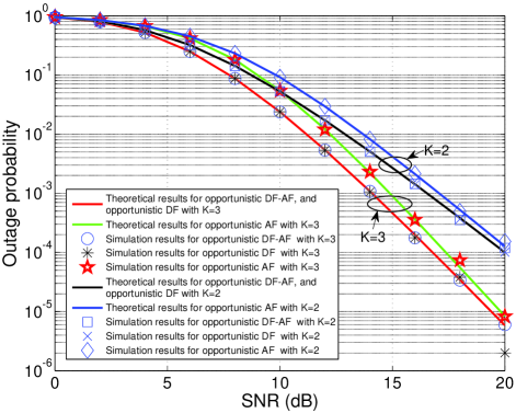
Figure 2: Outage probability in Rayleigh channels with $K$ relays

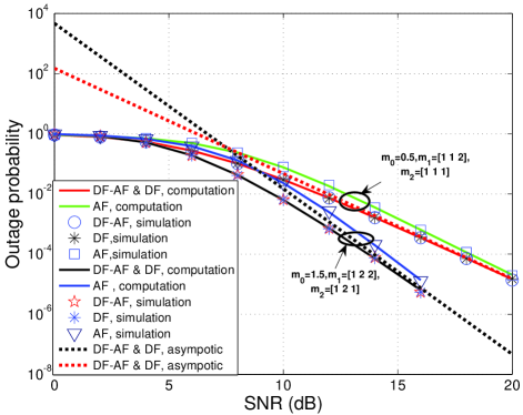
Figure 3: Outage probability in Nakagami-$m$ channels with 3 relays

Fig. 2 compares the outage probability obtained via simulations and theoretical evaluation with different number of potential cooperating relays ($K$) in Rayleigh fading environment ($m_{0}=m_{1i}=m_{2i}=1$). Fig. 3 compares the outage probability with general Nakagami-$m$ fading parameters in $K=3$ relays scenario, $m_{0}=0.5,m_{1}=[1~{}1~{}2],m_{2}=[1~{}1~{}1]$. As a benchmark, we also show the outage probability of the best-relay selection adaptive DF scheme [15] as well as the outage probability of the opportunistic AF schem. Observe that simulation curves match in high accuracy with analytical ones. When SC is utilized, opportunistic DF-AF scheme has the same outage probability as the best-relay selection adaptive DF scheme, which has better outage performance than the opportunistic AF scheme. The asymptotic outage coincides with the exact outage in high SNR region. We can notice that both the number of potential cooperating relays ($K$) and the fading parameters have a strong impact of the performance enhancement. We will analyze the impact of the relay number and the fading parameter respectively in the following.

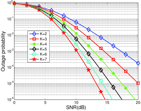
Figure 4: Outage probability with $K$ relays

Fig. 4 illustrates the theoretical results for the outage probability of opportunistic DF-AF scheme with different number of relays, $K$. In the computation, we set $m_{0}=0.8$ and $m_{1i}=m_{2i}=1$. When $m_{1i}=m_{2i}=1$, the diversity order is $d=m_{0}+K$ (See Fig. 5). From Fig. 4, we can clearly find that the number of relays impacts the slope of the curves. When there are more relays, the outage probability decreases more faster. In addition, the slopes of the curves in high SNR in Fig. 4 are concordant with the diversity order illustrated in Fig. 5.

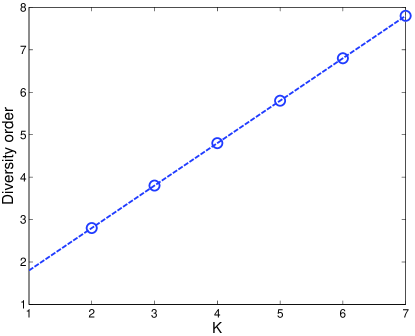
Figure 5: Diversity order with different $K$

Fig. 6 shows the diversity order with different channel fading parameters. We consider $2$ symmetric relays, i.e., $m_{1}=[g_{1}~{}g_{1}],m_{2}=[g_{2}~{}g_{2}]$. The fading parameter for the direct channel from the source to the destination is $m_{0}=0.5$. It can be observed that the diversity order is determined by the worse one in the source-relay channel ($g_{1}$) and relay-destination channel ($g_{2}$).

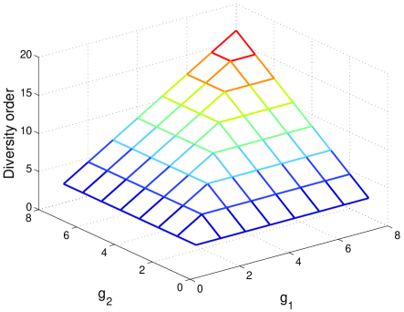
Figure 6: Diversity order with different fading parameters

To further demonstrate the advantages of the opportunistic DF-AF scheme, we show the outage performance of the three schemes when MRC is used in Fig. 7. The fading parameters are set as $m_{0}=0.5,m_{1}=[1~{}1~{}2],m_{2}=[1~{}1~{}1]$. Notice that the opportunistic DF-AF scheme has the best outage performance, which verifies the proposed theoretical analysis.

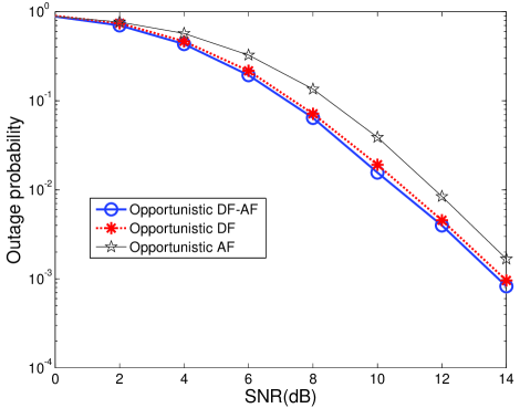
Figure 7: Outage comparison in 3-relay networks when MRC is applied

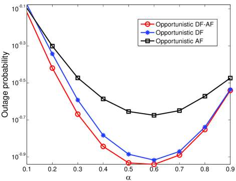
Figure 8: Outage comparison with different power allocations between the source and the relay in 3-relay networks, the total power $P_{s}+P_{r}=10~{}dB$ and the fading parameters are chosen as $m_{0}=0.5,m_{1}=[1~{}1~{}2],m_{2}=[1~{}1~{}1]$

In Fig. 8, we consider different power allocations between the source and the relay. Define $\alpha=P_{s}/(P_{s}+P_{r})$ as the power allocation coefficient, where $P_{s}$ and $P_{r}$ are the transmit power at the source and the relay, respectively. In the simulation, MRC is applied at the destination, and we set the AWGN variance $N_{0}=1$. From Fig. 8, we can see that the opportunistic DF-AF scheme outperforms the other two schemes. The advantages are obvious when $\alpha=0.2,...,0.7$, and the opportunistic DF-AF scheme has almost the same performance as the opportunistic DF scheme when $\alpha=0.8,0.9$. In addition, from the curve for the opportunistic DF-AF scheme, we can notice that with the increase of $\alpha$, the outage decreases at first and then increases. This can be explained as follows: When the source power increases, the relay has larger probability to correctly decode the source message, and then DF will be utilized with larger probability. Thus, the curves of the DF-AF scheme and DF scheme approach while we increase $\alpha$. The equivalent SNR of the relay path is given by (2). When the source power is low (i.e., $\alpha$ is small), the relay could not decode the source messages with high probability, equivalent SNR of the relay path is approximated by $\frac{\gamma_{1i}\gamma_{2i}}{\gamma_{1i}+\gamma_{2i}+1}$. In this case, the increase $\alpha$ will result in the increases of $\gamma_{1i}$ and decrease of $\gamma_{2i}$. Observe that $\gamma_{1i}$ increase from a small number and $\gamma_{2i}$ decreases from a large number, i.e., $\gamma_{1i}$ and $\gamma_{2i}$ approach each other. Consequently, $\frac{\gamma_{1i}\gamma_{2i}}{\gamma_{1i}+\gamma_{2i}+1}$ increases. Thus, we have better outage performance. However, when the source power goes beyond a threshold, the relay has high probability to decode the source messages, and the equivalent SNR of the relay path is determined by the SNR of the second hop $\gamma_{2i}$. The increase of $\alpha$ means the decrease of the relay power, i.e., the decrease of $\gamma_{2i}$. So we have higher outage probability. Finally, from the figure and the analysis, we can guess that an optimal $\alpha$ exists.

VI Conclusion

In this paper, we investigate the opportunistic DF-AF selection relaying scheme in wireless networks. The optimal relay selection for maximizing received destination SNR is studied. We analyze the outage probability over Nakagami-$m$ fading channels, and a closed-form solution is obtained. The coding gain and diversity order are derived whereby the asymptotic analysis in high SNR. We find that the diversity order depends on not only the relay number but also the fading parameters. Moreover, we prove that the opportunistic DF-AF selection relaying scheme outperforms both the opportunistic DF scheme and opportunistic AF scheme in terms of the outage performance. Finally, the numerical results verify our analysis. In addition, simulations demonstrate that the power allocation between the source and the relay plays an important role on the performance. We will investigate the the power allocation to further improve the performance in the future works.

References

• [1] A.ย Sendonaris, E.ย Erkip, and B.ย Aazhang, โ€œUser cooperation diversity-part I: system description,โ€ IEEE Trans. Commun., vol. 51, no. 11, pp. 1927-1938, Nov. 2003.
• [2] J.ย N. Laneman, D.ย N. C. Tse, and G.ย W. Wornell, โ€œCooperative diversity in wireless networks: efficient protocols and outage behavior,โ€ IEEE Trans. Inf. Theory, vol. 51, no. 12, pp. 3062-3080, Dec. 2004.
• [3] H. A. Suraweera, D. S. Michalopoulos and G. K. Karagiannidis, โ€œPerformance of distributed diversity systems with a single amplify-and-forward relay,โ€ IEEE Trans. Veh. Technol., vol. 58, pp. 2603-2608, June 2009.
• [4] M. R. Bhatnagar and A. Hj$\phi$rungnes, โ€œML decoder for decode-and-forward based cooperative communication system,โ€ IEEE Trans. Wireless Commun., vol. 10, no. 12, pp. 4080-4090, Dec. 2011.
• [5] B.ย Zhao and M.ย Valenti, โ€œSome new adaptive protocols for the wireless relay channel,โ€ Proc. Allerton Conf. Commun., Control, and Comp., Monticello, IL, Oct. 2003.
• [6] M. R. Souryal and B. R. Vojcic, โ€œPerformance of amplify-and-forward and decode-and-forward relaying in Rayleigh fading with turbo codes,โ€ย in Proc. IEEE ICASSP, Toulouse, France, May 2006.
• [7] Y. Li and B. Vucetic, โ€œOn the performance of a simple adaptive relaying protocol for wireless relay networks,โ€ Proc. of IEEE VTC-Spring 2008, Singapore.
• [8] W.ย Su, and X.ย Liu, โ€œOn optimum selection relaying protocols in cooperative wireless networks,โ€ IEEE Trans. Commun., vol. 58, no. 1, pp. 52-57, Jan. 2010.
• [9] A.ย Bletsas, A.ย Khisti, D. P. Reed, and A.ย Lippman, โ€œA simple cooperative diversity method based on network path selection,โ€ IEEE J. Sel. Areas Commun., vol. 24, no. 3, pp. 659-672, Mar. 2006.
• [10] E.ย Beres and R.ย Adve, โ€œSelection cooperation in multi-source cooperative networks, โ€ IEEE Trans. Wireless Commun., vol. 7, no. 2, pp. 118-127, Jan. 2009.
• [11] A.ย Bletsas, H.ย Shin and M.ย Z. Win, โ€œCooperative communications with outage-optimal opportunistic relaying,โ€ IEEE Trans. Wireless Commun., vol. 6, no. 9, pp. 3450-3460, Sept. 2007.
• [12] K.ย -S. Hwang,ย Y.-C. Ko, and M.ย -S. Alouini, โ€œOutage probability of cooperative diversity systems with opportunistic relaying based on decode-and-forward,โ€ IEEE Trans. Wireless Commun., vol. 7, no. 12, Dec. 2008.
• [13] M. M. Fareed and M. Uysal, โ€œOn relay selection for decode-and-forward relaying,โ€ IEEE Trans. Wireless Commun., vol. 8, no. 7, pp. 3341-3345, Jul. 2009.
• [14] Q.ย F. Zhou, F.ย C. M. Lau, and S.ย F. Hau, โ€œAsympotic analysis of opportunistic relaying protocols, โ€ IEEE Trans. Wireless Commun., vol. 8, no. 8, pp. 3915-3920, Aug. 2009.
• [15] S.ย S. Ikki and M.ย H. Ahmed, โ€œPerformance analysis of adaptive decode-and-forward cooperative diversity networks with best-relay selection,โ€ IEEE Trans. Commun., vol. 58, no. 1, pp. 68-72, Jan. 2010.
• [16] S.ย Savazzi and U.ย Spagnolini, โ€œCooperative space-time coded transmissions in Nakagami-$m$ fading channels,โ€ย  in Proc. IEEE GLOBECOMโ€™07, 2007, pp. 4334-4338.
• [17] T.ย A. Tsiftsis, G.ย K. Karagiannidis, P.ย T. Mathiopoulos, and S.ย A. Kotsopoulos, โ€œNonregenerative dual-hop cooperative links with selection diversity,โ€ EURASIP J. Wireless Commun. Networking, vol. 2006, article ID 17862, pp. 1-8, 2006.
• [18] P.ย A. Anghel and M.ย Kaveh, โ€œExact symbol error probability of a cooperative network in a Rayleigh-fading environment,โ€ IEEE Trans.Wireless Commun., vol. 3, no. 5, pp. 1416-1421, Sep. 2004.