Quantum Decoherence Scaling with Bath Size:
Importance of Dynamics, Connectivity, and Randomness

Abstract

The decoherence of a quantum system $S$ coupled to a quantum environment $E$ is considered. For states chosen uniformly at random from the unit hypersphere in the Hilbert space of the closed system $S+E$ we derive a scaling relationship for the sum of the off-diagonal elements of the reduced density matrix of $S$ as a function of the size $D_{E}$ of the Hilbert space of $E$. This sum decreases as $1/\sqrt{D_{E}}$ as long as $D_{E}\gg 1$. This scaling prediction is tested by performing large-scale simulations which solve the time-dependent Schrödinger equation for a ring of spin-$1/2$ particles, four of them belonging to $S$ and the others to $E$. Provided that the time evolution drives the whole system from the initial state toward a state which has similar properties as states belonging to the class of quantum states for which we derived the scaling relationship, the scaling prediction holds. For systems which do not exhibit this feature, it is shown that increasing the complexity (in terms of connections) of the environment or introducing a small amount of randomness in the interactions in the environment suffices to observe the predicted scaling behavior.

I Introduction

Decoherence of a quantum system $S$ interacting with a quantum environment $E$ is of importance for two reasons. First, decoherence of $S$ is the primary requirement for $S$ to relax to a state described by a canonical ensemble at a certain temperature Kubo et al. (1985). Second, decoherence is arguably the largest impediment for practical, realizable quantum computers Nielsen and Chuang (2000).

The large interest in technological areas like spintronics, quantum computing and quantum information processing have stimulated the theoretical research of quantum dynamics in open and closed interacting systems. Besides this more application driven interest there persists the fundamental and still unanswered question under which conditions a finite quantum system reaches thermal equilibrium and how this can be derived from dynamical laws.

On the one hand there exists a variety of studies exploring the microcanonical thermalization in an isolated quantum system Yukalov (2011); von Neumann (1929); Peres (1984); Deutsch (1991). On the other hand there exist various studies investigating the process of canonical thermalization of a system coupled to a (much) larger system Tasaki (1998); Goldstein et al. (2006); Popescu et al. (2006); Reimann (2007); Yukalov (2011); Linden et al. (2009); Short (2011); Reimann (2010) and of two finite identical quantum systems prepared at different temperatures Ponomarev et al. (2011, 2012).

In previous work Yuan et al. (2009); Jin et al. (2010), we numerically demonstrated that a quantum system interacting with an environment at high temperature relaxes to a state described by the canonical ensemble. In this paper we focus on investigating the dynamic properties of the decoherence of a quantum system $S$, being a subsystem of the whole system $S+E$. We do this both with a theoretical prediction and by simulating the dynamics of a relatively large system $S+E$ of spin-$1/2$ particles using a time-dependent Schrödinger equation (TDSE) solver De Raedt and Michielsen (2006). In particular, we investigate the scaling of the degree of decoherence of $S$ with the size of $E$, keeping the size of $S$ fixed. Based on similar arguments as given in Ref. Hams and De Raedt (2000), we find that the degree of decoherence of $S$ decreases as $1/\sqrt{D_{E}}$, where $D_{E}$ is the dimension of the Hilbert space of the environment if the state of the whole system is chosen uniformly at random from the unit hypersphere in the Hilbert space. In this paper, we denote states chosen uniformly at random from the unit hypersphere in the Hilbert space of the whole system by “$X$” and of the environment by “$Y$”.

We also address the question under what circumstances the whole system evolves to a state which has the same degree of decoherence as a state “$X$”. In particular we study the case in which the initial state of $S+E$ is a direct product of the state $\left|\uparrow\downarrow\uparrow\downarrow\right>$ of $S$ and a state “$Y$” of $E$. If the initial state of the whole system $S+E$ is slightly different from a given state “$X$”, the dynamics may drive the whole system into a state which is very different from the given state “$X$”, but which is of a similar type. We investigate through our simulations when the dynamics plays an important role in the decoherence in that it can drive $S+E$ to a state “$X$” by introducing small world bond connections in $E$ and/or between $S$ and $E$ and by introducing randomness in the interaction strengths of the environment.

The paper is organized as follows. In Section II our theoretical results for the scaling of the decoherence of $S$ are presented, together with details of the one-dimensional ring of spin-$1/2$ particles which we simulate to better understand the scaling prediction. Sections III-V contain results for the one-dimensional rings under study. In particular we look at the effect of adding additional bonds (Small World Bonds, SWBs) between the system and environment spins and/or between environment spins only (Section IV) and of randomness in the interaction strengths of the Hamiltonian of the environment (Section V). Section VI contains our conclusions and a discussion of our results.

II Theory, Model, and Methods

The time evolution of a closed quantum system is governed by the time-dependent Schrödinger equation (TDSE) von Neumann (1955); Ballentine (2003). If the initial density matrix of an isolated quantum system is non-diagonal then, according to the time evolution dictated by the TDSE, it remains non-diagonal. Therefore, in order to decohere the system $S$, it is necessary to have the system $S$ interact with an environment $E$, also called a heat bath or spin bath if the environment is composed of spins. Thus, the Hamiltonian of the whole system $S+E$ takes the form

$$H=H_{S}+H_{E}+H_{SE}\>,$$ (1)

where $H_{S}$ and $H_{E}$ are the system and environment Hamiltonian respectively, and $H_{SE}$ describes the interaction between the system and environment. In what follows, we first describe the general theory that leads to the scaling of the decoherence of the system $S$ with the size of $E$ and $S$. We then describe in detail the spin-$1/2$ Hamiltonians we have simulated to provide a case study for this scaling.

II.1 Time evolution

A pure state of the whole system $S+E$ evolves in time according to (in units of $\hbar=1$)

$$\left|\Psi(t)\right\rangle = e^{-itH}\left|\Psi(0)\right\rangle=\sum_{i=1}^{D_{S}}\sum_{p=1}^{D_{E}}c(i,p,t)\left|i,p\right\rangle\>,$$ (2)

where the set of states $\{|i,p\rangle\}$ denotes a complete set of orthonormal states in some chosen basis, and $D_{S}$ and $D_{E}$ are the dimensions of the Hilbert spaces of the system and the environment, respectively. We assume that $D_{S}$ and $D_{E}$ are both finite.

The spin Hamiltonian $H$ models a system with $N_{S}$ spin-$1/2$ particles and an environment with $N_{E}$ spin-$1/2$ particles. Thus, $D_{S}=2^{N_{S}}$ and $D_{E}=2^{N_{E}}$. The whole system $S+E$ contains $N=N_{S}+N_{E}$ spin-$1/2$ particles and the dimension of its Hilbert space is $D=D_{S}D_{E}$. In our simulations we use the spin-up – spin-down basis. Numerically, the real-time propagation by $e^{-itH}$ is carried out by means of the Chebyshev polynomial algorithm Tal-Ezer and Kosloff (1984); Leforestier et al. (1991); Iitaka et al. (1997); Dobrovitski and De Raedt (2003), thereby solving the TDSE for the whole system starting from the initial state $\left|\Psi(0)\right\rangle$. This algorithm yields results that are very accurate (close to machine precision), independent of the time step used De Raedt and Michielsen (2006).

II.2 Computational aspects

Computer memory and CPU time severely limit the sizes of the quantum systems that can be simulated. The required CPU time is mainly determined by the number of operations to be performed on the spin-$1/2$ particles. The CPU time does not put a hard limit on the simulation. However, the memory of the computer does severely limit which system sizes can be calculated. The state $\left|\Psi\right\rangle$ of a $N$-spin-$1/2$ system is represented by a complex-valued vector of length $D=2^{N}$. In view of the potentially large number of arithmetic operations, it is advisable to use 13 - 15 digit floating-point arithmetic (corresponding to 8 bytes for a real number). Thus, to represent a state of the quantum system of $N$ spin-$1/2$ particles on a conventional digital computer, we need a least $2^{N+4}$ bytes. Hence, the amount of memory that is required to simulate a quantum system with $N$ spin-$1/2$ particles increases exponentially with $N$. For example, for $N=24$ ($N=36$) we need at least 256 MB (1 TB) of memory to store a single arbitrary state $\left|\Psi\right\rangle$. In practice we need three vectors, memory for communication buffers, local variables and the code itself.

The elementary operations performed by the computational kernel are of the form $\left|\Psi\right\rangle\leftarrow U\left|\Psi\right\rangle$ where $U$ is a sparse unitary matrix with a very complicated structure (relative to the computational basis). Inherent to the problem at hand is that each operation $U$ affects all elements of the state vector $\left|\Psi\right\rangle$ in a nontrivial manner. This translates into a complicated scheme for accessing memory, which in turn requires a sophisticated MPI communication scheme De Raedt et al. (2007).

II.3 Reduced density matrix

The state of the quantum system $S$ is described by the reduced density matrix

$$\hat{\rho}(t)\equiv\mathbf{Tr}_{E}\rho\left(t\right)\>,$$ (3)

where $\rho\left(t\right)$ is the density matrix of the whole system $S+E$ at time $t$ and $\mathbf{Tr}_{E}$ denotes the trace over the degrees of freedom of the environment. In terms of the expansion coefficients $c(i,p,t)$, the matrix element $(i,j)$ of the reduced density matrix reads

$$\hat{\rho}_{ij}(t) = \mathbf{Tr}_{E}\sum_{p=1}^{D_{E}}\sum_{q=1}^{D_{E}}c^{\ast}(i,q,t)c(j,p,t)|j,p\rangle\langle i,q|$$ (4)

$$= \sum_{p=1}^{D_{E}}c^{\ast}(i,p,t)c(j,p,t)\>.$$

We characterize the degree of decoherence of the system by

$$\sigma(t)=\sqrt{\sum_{i=1}^{D_{S}-1}\sum_{j=i+1}^{D_{S}}\left|\widetilde{\rho}_{ij}(t)\right|^{2}}\>,$$ (5)

where $\widetilde{\rho}_{ij}(t)$ is the matrix element $(i,j)$ of the reduced density matrix $\widetilde{\rho}$ in the representation that diagonalizes $H_{S}$. Clearly, $\sigma(t)$ is a global measure for the size of the off-diagonal terms of the reduced density matrix in the representation that diagonalizes $H_{S}$. If $\sigma(t)=0$ the system is in a state of full decoherence (relative to the representation that diagonalizes $H_{S}$).

II.4 Scaling property of $\sigma$

We can prove a scaling property of $\sigma$ by assuming that the final state of the whole system is a state “$X$”, a state that is picked uniformly at random from the unit hypersphere in the Hilbert space. The wave function of the whole system reads,

$$\left|\Psi\right>=\sum_{i=1}^{D_{S}}\sum_{p=1}^{D_{E}}C_{i,p}\left|E_{i}^{(S)}\right>\left|E_{p}^{(E)}\right>,$$ (6)

where $\left\{\left|E_{i}^{(S)}\right\rangle\right\}$ $\left(\left\{\left|E_{p}^{(E)}\right\rangle\right\}\right)$ is the set of eigenvectors of $H_{S}$ ($H_{E}$), and the real and imaginary parts of $C_{i,p}$ are real random variables. The derivation of the scaling behavior follows Ref. Hams and De Raedt (2000). In particular Eqs. (A8), (A12) and (A23) of Ref. Hams and De Raedt (2000) are used. We introduce the following shorthand notation for the sum over the off-diagonal elements, $\sum_{i\neq j}^{D_{S}}\kappa_{ij}=\sum_{i=1}^{D_{S}}\sum_{j=1}^{D_{S}}\left(1-\delta_{ij}\right)\kappa_{ij}$ for any $\kappa_{ij}$, where $\delta_{ij}$ is the Kronecker delta function. The expectation value is given by

$$E\left(2\sigma^{2}\right) = E\left(\sum_{i\neq j}^{D_{S}}\left|\sum_{p=1}^{D_{E}}C_{i,p}^{*}C_{j,p}\right|^{2}\right)=\sum_{i\neq j}^{D_{S}}\>\sum_{p=1,p^{\prime}=1}^{D_{E}}E\left(C_{i,p}^{*}C_{j,p}C_{i,p^{\prime}}C_{j,p^{\prime}}^{*}\right)$$ (7)

$$= \sum_{i\neq j}^{D_{S}}\>\sum_{p=1,p^{\prime}=1}^{D_{E}}\left(\left(1-\delta_{p,p^{\prime}}\right)E\left(C_{i,p}^{*}C_{j,p}C_{i,p^{\prime}}C_{j,p^{\prime}}^{*}\right)+\delta_{p,p^{\prime}}E\left(C_{i,p}^{*}C_{j,p}C_{i,p^{\prime}}C_{j,p^{\prime}}^{*}\right)\right)$$ (8)

$$= \sum_{i\neq j}^{D_{S}}\sum_{p=1}^{D_{E}}E\left(\left|C_{i,p}\right|^{2}\left|C_{j,p}\right|^{2}\right)=\sum_{i\neq j}^{D_{S}}\sum_{p=1}^{D_{E}}\frac{1}{D_{S}D_{E}\left(D_{S}D_{E}+1\right)}=\frac{D_{S}-1}{D_{S}D_{E}+1}=\frac{1-\frac{1}{D_{S}}}{D_{E}+\frac{1}{D_{S}}}\>,$$ (9)

where $E(\cdot)$ denotes the expectation value with respect to the probability distribution of the random variables $C_{i,p}$. Equation (7) does not require any condition on the Hamiltonian Eq. (1). For example, if $H_{E}$ is composed of two or more environments that do not couple to each other, but only interact with the system, in Eq. (7) $D_{E}$ is the product of the sizes of the Hilbert spaces of all the environments. In addition, Eq. (7) does not impose any requirement on the geometry.

From Eq. (7) it follows that for any fixed value of $D_{S}>1$ and $D_{E}\gg 1$, $\sigma$ scales as

$$\sigma\approx\frac{1}{\sqrt{2}}\sqrt{E\left(2\sigma^{2}\right)}=\frac{1}{\sqrt{2}}\sqrt{\frac{D_{S}-1}{D_{S}D_{E}+1}}\sim\frac{1}{\sqrt{2D_{E}}}\>.$$ (10)

Therefore, if the size of the system $S$ is fixed (which is the case considered in this paper), $\sigma$ decreases as $1/\sqrt{D_{E}}$ for large $D_{E}$. Hence, for a spin-$1/2$ system $\sigma$ should decrease as $2^{-N_{E}/2}$ for large $N_{E}$.

For fixed $D_{S}>1$, it follows from Eq. (7) that the environment does not have to be very large for Eq. (10) to hold, which is in agreement with Ref. Gemmer and Michel (2006). Nevertheless, the existence of an environment is crucial. If there is no environment, then the $\sigma$ approaches to a constant (see Appendix A), even if the whole system is initially in a state “$X$”.

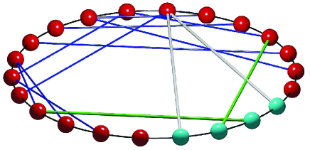
Figure 1: (Color online) An example of a spin system used in the simulations. The $N_{S}=4$ system spin-$1/2$ particles are colored light gray (cyan), and the $N_{E}=18$ environment spin-$1/2$ particles are colored dark gray (red). The thin black segments show the connections for a one-dimensional ring, which are the only bonds (interactions) present in case I and II (see text). The thick (green and white) bonds show SWBs in $H_{SE}$. This particular example shows a spin system with $K=2$, where $K$ denotes the maximum number of subsystem spins that are connected via SWBs with one environment spin (thick white lines, see also Section IV). The medium thick (blue) bonds show SWBs in $H_{E}$.

II.5 Model and method

For testing the predicted scaling of Eq. (10) we simulate systems of spin-$1/2$ particles. For studying the time evolution of the whole system $S+E$, we consider a general quantum spin-$1/2$ model defined by the Hamiltonian of Eq. (1) where

$$H_{S} = -\sum_{i=1}^{N_{S}-1}\sum_{j=i+1}^{N_{S}}\sum_{\alpha=x.y,z}J_{i,j}^{\alpha}S_{i}^{\alpha}S_{j}^{\alpha},$$ (11)

$$H_{E} = -\sum_{i=1}^{N_{E}-1}\sum_{j=i+1}^{N_{E}}\sum_{\alpha=x,y,z}\Omega_{i,j}^{\alpha}I_{i}^{\alpha}I_{j}^{\alpha},$$ (12)

$$H_{SE} = -\sum_{i=1}^{N_{S}}\sum_{j=1}^{N_{E}}\sum_{\alpha=x,y,z}\Delta_{i,j}^{\alpha}S_{i}^{\alpha}I_{j}^{\alpha}.$$ (13)

Here, $S$ and $I$ denote the spin-$1/2$ operators of the spins of the system and the environment, respectively (we use units such that $\hbar$ and $k_{B}$ are one). The spin components $S^{\alpha}_{i}$ and $I^{\alpha}_{j}$ are related to the Pauli spin matrices, for example $S^{x}_{i}$ is a direct product of identity matrices and the Pauli spin matrix $\frac{1}{2}\sigma^{x}=\frac{1}{2}\left(\begin{array}[]{cc}0&1\cr 1&0\end{array}\right)$ in position $i$ of the direct product with $1\leq i\leq N_{S}$.

For the geometry of the whole system, we focus on the one-dimensional ring consisting of a system with $N_{S}=4$ spin-$1/2$ particles and an environment with $N_{E}$ spin-$1/2$ particles, see Fig. 1. Past simulations have shown that a high connectivity spin-glass type of environment is extremely efficient to decohere a system Yuan et al. (2006, 2009); Yuan (2011); Brox et al. (2012), so we may expect that the one-dimensional ring is one of the most difficult geometries to obtain decoherence in short times.

We assume that the spin-spin interaction strengths of the system $S$ are isotropic, $J_{i,j}^{\alpha}=J$ and that only the nearest-neighbor interaction strengths $\Omega_{i,j}^{\alpha}$ and $\Delta_{i,j}^{\alpha}$ are non-zero. Note that for a ring there are only two bonds with strength $\Delta_{i,j}^{\alpha}$ connecting $S$ and $E$. We distinguish two cases:

• Case I: The non-zero values of $\Omega_{i,j}^{\alpha}$ and $\Delta_{i,j}^{\alpha}$ are generated uniformly at random from the range $[-\Omega,\Omega]$ and $[-\Delta,\Delta]$, respectively.

• Case II: All non-zero values of the model parameters are identical, $\Omega_{i,j}^{\alpha}=J$ and $\Delta_{i,j}^{\alpha}=J$. This corresponds to a uniform isotropic Heisenberg model with interaction strength $J$.

We will see that these two cases show very different scaling properties of the decoherence depending on the initial state. We also investigate the effects of randomly adding small world bonds (SWBs) between spins in the system and environment and between spins in the environment (see Fig. 1).

The initial state of the whole system $S+E$ is prepared in two different ways, namely:

• “$X$”: We generate Gaussian random numbers $\{a(j,p),b(j,p)\}$ and set $c(j,p,t=0)=(a(j,p)+ib(j,p))/\sqrt{\sum_{j,p}(a^{2}(j,p)+b^{2}(j,p))}$. Clearly this procedure generates a point on the hypersphere in the $D$-dimensional Hilbert space. Alternatively, we generate points in the hypercube by using uniform random numbers in the interval $[-1,1]$. Our general conclusions do not depend on the procedure used (results not shown).

• $UDUDY$: The initial state of the whole system is a product state of the system and environment. In this paper ($N_{S}=4$), we confine the discussion to the state $UDUDY$, which means that the first, second, third, and fourth spin are in the up, down, up, and down state respectively, and the state of the remaining spins is a “$Y$” state in the $(D/2^{4})$-dimensional Hilbert space. The “$Y$” state of the environment is prepared in the same way as the “$X$” state of the whole system.

III Scaling analysis of $\sigma$

All simulations are carried out for a system $S$ consisting of four spins ($N_{S}=4$) coupled to an environment $E$ with the number of spins $N_{E}$ ranging from $2$ to $30$. The interaction strengths $J_{i,i+1}^{\alpha}$ with $1\leq i\leq N_{S}-1$ are always fixed to $J=-0.15$. For case I all non-zero $\Omega_{i,j}^{\alpha}$ and $\Delta_{i,j}^{\alpha}$ are randomly generated from the range $[-0.2,0.2]$. For case II all non-zero $\Omega_{i,j}^{\alpha}$ and $\Delta_{i,j}^{\alpha}$ are equal to $J=-0.15$ (isotropic Heisenberg model).

III.1 Verification of scaling: cases I and II with “$X$”

Figure 2: Simulation results for $\sigma(t)$ (see Eq. (5)) for case I (top) and case II (bottom) for different sizes $N=N_{E}+4$ of the whole system. The initial state of the whole system is “$X$” (see text). Curves from top to bottom correspond to system sizes ranging from $N=6$ to $N=34$ in steps of $2$. The insets show the time-averaged values of $\sigma(t)$ (pluses) as a function of the size $N_{E}$ of the environment, confirming the theoretical prediction of Eq. (10) (solid line).

We corroborate the scaling property of Eq. (10) by numerically simulating the quantum spin system (see Eq. (11) through (13)). If we choose the initial state of the whole system to be an “$X$” state, then during the time evolution the whole system will remain in the state “$X$”. Hence, the condition to derive Eq. (10) are fulfilled. Fig. 2 demonstrates that the numerical results for both cases I and II agree with Eq. (10). In particular the insets in Fig. 2 show that for both cases I and II, $\ln(2\sigma)\approx-N_{E}/2$, and that $\sigma$ scales as $1/\sqrt{D_{E}}$ even if $N_{E}=2$ and $N_{S}=4$ ($N_{E}<N_{S}$).

III.2 Different initial conditions

We investigate the effects of the dynamics by preparing the initial state of the whole system such that it is slightly different from “$X$”. The initial state of the whole system is set to $UDUDY$. In contrast to Fig. 2, we will see that the two cases I and II behave differently.

III.2.1 Case I and $UDUDY$

Figure 3: Simulation results for $\sigma(t)$ (see Eq. (5)) for case I for different sizes $N=N_{E}+4$ of the whole system. The initial state of the whole system is $UDUDY$ (see text). Curves from top to bottom correspond to system sizes ranging from $N=6$ to $N=34$ in steps of $2$. The inset shows the time-averaged values of $\sigma(t)$ (pluses) as a function of the size $N_{E}$ of the environment. The data obey the scaling property of Eq. (10) (solid line).

In Fig. 3, we present the simulation results for case I, the couplings in the Hamiltonians $H_{E}$ and $H_{SE}$ are chosen uniformly at random. The size $N=N_{E}+4$ of the whole system ranges from $6$ to $34$. An average over the long-time stationary steady-state values of $\sigma(t)$ still obeys the scaling property of Eq. (10), showing that $\sigma$ decreases as $1/\sqrt{D_{E}}$, where $D_{E}=2^{N_{E}}$. If $N_{E}\rightarrow\infty$, $\sigma\rightarrow 0$. This suggests that in the thermodynamical limit the system $S$ decoheres completely.

III.2.2 Case II and $UDUDY$

Figure 4: Same as Fig. 3 for case II instead of case I. Curves from top to bottom correspond to system sizes ranging from $N=16$ to $N=34$ in steps of $2$. The solid line in the inset is a guide to the eyes.

We consider the case in which the whole system is described by the isotropic Heisenberg model ($J^{\alpha}_{i,i+1}=\Omega^{\alpha}_{i,i+1}=\Delta^{\alpha}_{i,i+1}=J$). In Fig. 4 we present simulation results for different system sizes $N=N_{E}+4$ ranging from $16$ to $34$. From Fig. 4, it is seen that the behavior for case II is totally different from that of case I (see Fig. 3). In particular, $\sigma(t)$ does not scale with the dimension of the environment. From the present numerical results, we cannot make any conclusions about the limit for large $N_{E}$. However if $\sigma(t)$ approaches zero as $N_{E}\rightarrow\infty$ (see the fifth column of Table 1) it does so very slowly.

III.3 Computational effort

In this paper, the largest number of spins that we simulated is $N=34$. Using the Chebyshev polynomial algorithm and a large time step ($\tau\approx 10\pi$), the $N=34$ simulation for the bottom curves in Fig. 2 (up to a time $t\approx 600$) took about $0.3$ million core hours on $16384$ BG/P (IBM Blue Gene P) processors, using $1024$ GB of memory. Similarly, it took about $4$ million core hours to complete the $N=34$ curve in Fig. 3 (up to a time $t\approx 8000$).

III.4 Summary: initial state dependence

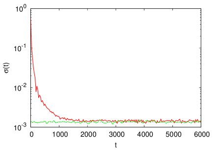
Figure 5: (Color online) Simulation results for $\sigma(t)$ for case I for $N=22$ and $N_{S}=4$. Red solid line: the initial state is $UDUDY$ (see text); green dashed line: the initial state is “$X$” (see text).

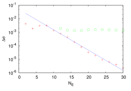
Figure 6: (Color online) Difference $\Delta\sigma$ between the time-averaged values of $\sigma(t)$ for the initial state $UDUDY$ and “$X$” of the whole system (see Table 1) as a function of the size of the environment $N_{E}$. Pluses: case I; circles: case II. The dotted line is a linear fit to the data (pluses) for the $UDUDY$ initial state, excluding the first three data points, resulting in $\Delta\sigma=0.049/\sqrt{D_{E}}$.

Table 1: The time average of $\sigma(t)$ in the stationary regime shown in Figs. 2, 3 and 4.

	prediction	case I		case II
$N_{E}$	of Eq. (10)	$UDUDY$	“$X$”	$UDUDY$	“$X$”
2	$3.397\times 10^{-1}$	$3.416\times 10^{-1}$	$3.375\times 10^{-1}$		$3.334\times 10^{-1}$
4	$1.708\times 10^{-1}$	$1.746\times 10^{-1}$	$1.727\times 10^{-1}$		$1.711\times 10^{-1}$
6	$8.554\times 10^{-2}$	$8.834\times 10^{-2}$	$8.536\times 10^{-2}$		$8.492\times 10^{-2}$
8	$4.279\times 10^{-2}$	$4.598\times 10^{-2}$	$4.282\times 10^{-2}$		$4.265\times 10^{-2}$
10	$2.139\times 10^{-2}$	$2.286\times 10^{-2}$	$2.153\times 10^{-2}$		$2.121\times 10^{-2}$
12	$1.070\times 10^{-2}$	$1.149\times 10^{-2}$	$1.071\times 10^{-2}$	$1.254\times 10^{-2}$	$1.061\times 10^{-2}$
14	$5.349\times 10^{-3}$	$5.795\times 10^{-3}$	$5.357\times 10^{-3}$	$6.756\times 10^{-3}$	$5.346\times 10^{-3}$
16	$2.674\times 10^{-3}$	$2.866\times 10^{-3}$	$2.678\times 10^{-3}$	$3.997\times 10^{-3}$	$2.663\times 10^{-3}$
18	$1.337\times 10^{-3}$	$1.430\times 10^{-3}$	$1.349\times 10^{-3}$	$2.694\times 10^{-3}$	$1.343\times 10^{-3}$
20	$6.686\times 10^{-4}$	$7.065\times 10^{-4}$	$6.736\times 10^{-4}$	$2.204\times 10^{-3}$	$6.641\times 10^{-4}$
22	$3.343\times 10^{-4}$	$3.542\times 10^{-4}$	$3.352\times 10^{-4}$	$1.909\times 10^{-3}$	$3.347\times 10^{-4}$
24	$1.672\times 10^{-4}$	$1.766\times 10^{-4}$	$1.674\times 10^{-4}$	$1.722\times 10^{-3}$	$1.658\times 10^{-4}$
26	$8.358\times 10^{-5}$	$9.005\times 10^{-5}$	$8.368\times 10^{-5}$	$1.599\times 10^{-3}$	$8.283\times 10^{-5}$
28	$4.179\times 10^{-5}$	$4.551\times 10^{-5}$	$4.151\times 10^{-5}$	$1.481\times 10^{-3}$	$4.176\times 10^{-5}$
30	$2.089\times 10^{-5}$	$2.338\times 10^{-5}$	$2.107\times 10^{-5}$	$1.379\times 10^{-3}$	$2.104\times 10^{-5}$

For an initial state “$X$” of the whole system the scaling of $\sigma$, as given by Eq. (10), works extremely well for both case I and case II, as seen in Fig. 2. When the initial state is $UDUDY$, we can understand the very different behavior of cases  I and II, see Figs. 3 and 4, by considering the stationary states that are obtained. Figure 5 shows that the final values of $\sigma(t)$ for case I are very close for both initial states “$X$” and $UDUDY$. This suggests that the final stationary state in case I has properties similar to those of a state “$X$”, and hence case I obeys the scaling property of Eq. (10) to a good approximation. The time-averaged values of $\sigma(t)$ in Figs. 2, 3 and 4, denoted by $\overline{\sigma}$, are listed in Table 1. From Table 1, we see that the values of $\overline{\sigma}$ for case II with an initial state $UDUDY$ are very different from those with an initial state “$X$”, and do not show the scaling property of Eq. (10). Thus, the numerical results suggest that the initial state and the randomness of the interaction strengths play a very important role in the dynamical evolution of the decoherence of a system coupled to an environment. In particular, for case II, starting from a state “$X$” the time-averaged values of $\sigma(t)$ scale as $\overline{\sigma}\approx 1/\sqrt{D_{E}}$, but such scaling is not observed for starting from a state $UDUDY$.

From Table 1, it is seen that the values of $\overline{\sigma}$ for case I with the initial state $UDUDY$ are always slightly larger than those with the initial state “$X$”. Therefore, it is interesting to examine the difference $\Delta\sigma$ between the values of $\overline{\sigma}$ for the initial states $UDUDY$ and “$X$”. Figure 6 shows that $\Delta\sigma$ for case I (red pluses) also scales as $1/\sqrt{D_{E}}$ (dotted line), except for the first three data points, which is probably due to large fluctuations in the calculations for these small system sizes. Therefore, the dynamics of case I will drive the system to a state “$X$” only when the environment approaches infinity. Figure 6 also shows that $\Delta\sigma$ for case II (circles) is almost constant for system sizes $N$ ranging from $16$ to $34$. Hence, it is unlikely that case II with the initial state $UDUDY$ will decohere, even if the simulations could be performed for much longer times and for larger system sizes.

IV Connectivity: ring with small world bonds

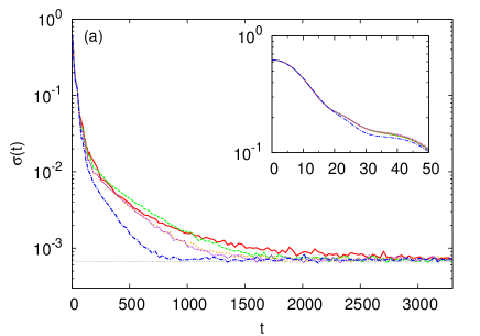
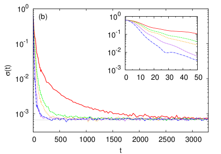
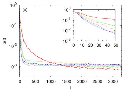
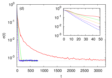
Figure 7: (Color online) Simulation results of $\sigma(t)$ for case I with $N=24$ and $N_{S}=4$ with SWBs added. The initial state is $UDUDY$. The dotted horizontal line represents the value of Eq. (10). Red solid line: ring without SWBs. (a) Randomly added SWBs between non-neighboring environment spins. Green long-dashed line: one SWB; orange dotted line: two SWBs; purple short-dashed line: four SWBs; blue dotted-dashed line: eight SWBs. (b) Randomly added SWBs between the system and environment spins such that $K=1$. Green long-dashed line: one SWB; orange dotted line: two SWBs; purple short-dashed line: four SWBs; blue dotted-dashed line: eight SWBs. (c) Randomly added SWBs between the system and environment spins such that $K=2$. Green long-dashed line: two SWBs; orange dotted line: four SWBs; purple short-dashed line: six SWBs; blue dotted-dashed line: eight SWBs. (d) Same as (c) except that each pair of non-neighboring environment spins is connected by a SWB. Insets: time evolution for short times.

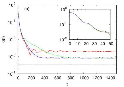
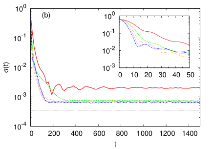
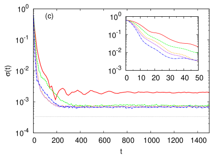
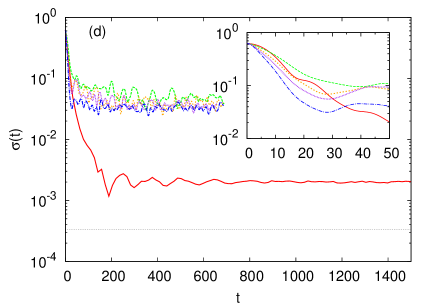
Figure 8: (Color online) Simulation results of $\sigma(t)$ for case II with $N=26$ and $N_{S}=4$ with isotropic SWBs added. The initial state is $UDUDY$. The dotted horizontal line represents the value of Eq. (10). Red solid line: ring without SWBs. (a) Randomly added SWBs between non-neighboring environment spins. Green long-dashed line: two SWBs; orange dotted line: four SWBs; purple short-dashed line: six SWBs; blue dotted-dashed line: eight SWBs. (b) Randomly chosen SWBs between the system and environment spins such that $K=1$. Green long-dashed line: two SWBs; orange dotted line: four SWBs; purple short-dashed line: six SWBs; blue dotted-dashed line: eight SWBs. (c) Randomly chosen SWBs between the system and environment spins such that $K=2$. Green long-dashed line: two SWBs; orange dotted line: four SWBs; purple short-dashed line: six SWBs; blue dotted-dashed line: eight SWBs. (d) Same as (c) except that each pair of non-neighboring environment spins is connected by a SWB. Insets: time evolution for short times.

We investigate the effects of adding small world bonds (SWBs) to the Hamiltonians $H_{SE}$ or/and $H_{E}$ for both case I and case II (see Fig. 1). To analyze the addition of SWBs to $H_{SE}$ we distinguish between spin systems with $K<2$ and $K\geq 2$, where $K$ denotes the maximum number of subsystem spins that are connected via SWBs with one environment spin. This distinction is motivated by the distinct decoherence characteristics for systems with $K<2$ and $K\geq 2$ for case I (see next subsection). An example of a spin configuartion with $K=2$ is shown in Fig. 1. In particular, we are interested in whether systems with SWBs will exhibit the same scaling, and whether they will decohere from an initial state faster than either of the cases studied thus far. The addition of many SWBs changes the graph from a one-dimensional ring to a graph with equal bond lengths that can only be embedded in high dimensions. The initial states are always $UDUDY$. Furthermore, in order not to change too many parameters simultaneously we start all simulations from the same state “$Y$” of the environment. Furthermore, after choosing the random location (and couplings $\Omega^{\alpha}$ and $\Delta^{\alpha}$ for case I) of the first SWB we preserve this bond when adding additional SWBs. We will see that case I and case II still behave very differently.

IV.1 Case I and SWBs

For investigating the universality of the final value of $\sigma(t)$ we add SWBs (random couplings in the interval $[-0.2,0.2]$) in the Hamiltonian $H_{SE}$ or/and $H_{E}$ for case I, and perform simulations for $N=24$ with $N_{S}=4$. From Fig. 7a, we see that adding more and more SWBs to $H_{E}$ speeds up the decoherence process and that the final value of $\sigma(t)$ corresponds to the one given by Eq. (10). As seen in the inset, adding SWBs to $H_{E}$ has no noticeable effect on the early time behavior of $\sigma(t)$.

Adding SWBs exclusively to $H_{SE}$ speeds up the decoherence process even further and even at early times clear changes in $\sigma(t)$ can be observed (see Figs. 7b, c). For spin configurations with $K=1$, $\sigma(t)$ reaches the value given by Eq. (10) for sufficiently long times, as can be seen from Fig. 7b. However, for configurations with $K=2$ (see Fig. 7c) or $K>2$ (results not shown) $\sigma(t)$ does not obey the scaling property Eq. (10). Restoring this scaling property seems to require an environment that is much more complex than the one-dimensional one as indicated by Fig. 7d in which we present simulation results for the case that SWBs between all non-neighboring environment spins have been added.

IV.2 Case II and SWBs

For case II, isotropic SWBs are added to $H_{SE}$ or/and $H_{E}$. From Fig. 8, it is clear that even for long times none of the curves approach the dotted horizontal line, the value of $\sigma(t)$ for an initial state “$X$”. Adding SWBs exclusively to $H_{E}$ does not have a dramatic effect on $\sigma(t)$ and has very little effect at early times (see Fig. 8a).

Just as for case I, it is seen that adding a few SWBs exclusively to $H_{SE}$ for a spin configuration with $K=1$ significantly decreases the time to approach the steady state, and that the SWBs in $H_{SE}$ also lead to a decrease in $\sigma(t)$ for a fixed time even at early times (see Fig. 8b). For spin configurations with $K=2$ case I and case II seem to have similar decoherence properties if SWBs are added exclusively to $H_{SE}$, as seen by comparing Fig. 7c and Fig. 8c. However, connecting in addition each pair of non-neighboring environment spins by isotropic SWBs drives the curves very far away from the value of $\sigma(t)$ for an initial state “$X$” (see Fig. 8d).

IV.3 Summary: SWBs

Adding SWBs to $H_{SE}$ or/and to $H_{E}$ changes the rate of decoherence as seen by the approach to the asymptotic value for $\sigma(t)$. In case II, adding isotropic SWBs to $H_{SE}$ or $H_{E}$ effectively alters some spin-spin correlations leading to a decrease in the steady-state value of $\sigma(t)$. However, this decrease is not sufficient to reach the steady-state value of $\sigma(t)$ that complies with the prediction Eq. (10). Adding isotropic SWBs to $H_{SE}$ and connecting in addition each pair of non-neighboring environment spins by isotropic SWBs drives the curves very far away from the value of $\sigma(t)$ for an initial state “$X$”, even much further away than the steady-state value for a ring without SWBs. In contrast to case I systems with $K<2$ and $K\geq 2$ do not behave significantly different.

Comparing case II with case I for $K<2$, we conclude that without introducing the randomness in the $x,$ $y,$ $z$ components of the spin-spin couplings, the dynamics cannot drive the system to decoherence if the initial state is different from a state “$X$”. Increasing the complexity of the environment by adding isotropic SWBs between all non-neighboring environment spins does not help in this respect, even on the contrary. However, for case I and configurations with $K\geq 2$, increasing the complexity of the environment by adding SWBs between all pairs of non-neighboring environment spins allows the dynamics to drive the system to decoherence.

For both case I and case II, adding SWBs in $H_{SE}$ and $H_{E}$ separately speeds up the decoherence in that it evolves more quickly to a stationary state. The asymptotic value for $\sigma(t)$ is approached much faster when adding SWBs to $H_{SE}$ instead of $H_{E}$, and the SWBs in $H_{SE}$ also affect $\sigma(t)$ at early times. Thus a random SWB coupling to the system via $H_{SE}$ is the most effective way to decrease the time for decoherence.

V Randomness in the environment

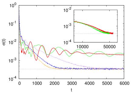
Figure 9: (Color online) Simulation results of $\sigma(t)$ obtained by selectively replacing isotropic spin-spin interactions by random bonds. The size of the system and whole system are $N_{S}=4$ and $N=26$, respectively. The initial state is $UDUDY$. Red solid line: $1$ random bond; green long-dashed line: $2$ random bonds; purple dotted line: $4$ random bonds; orange short-dashed line: $6$ random bonds; blue dotted-dashed line: $8$ random bonds. Inset: simulation results for one and two random bonds for long times.

Section III.1 shows that for the initial state “$X$” the scaling predicted by Eq. (10) is confirmed both for case I and case II (see Fig. 2). However, section III.2 shows that starting from the initial state $UDUDY$ this scaling is approached as $1/\sqrt{D_{E}}$ for case I (see Figs. 3 and 6) but not for case II (see Figs. 4 and 6). Section IV shows that adding SWBs in case II does not significantly change the long-time behavior of $\sigma(t)$ approaching the predicted value of Eq. (10). Therefore the natural question to ask is how much randomness is required for $\sigma(t)$ to obey the scaling relation Eq. (10). To answer this question, we start from the isotropic Heisenberg ring (case II) and replace the interaction strengths of a few randomly chosen bonds by random $\Omega_{i,j}^{\alpha}$ (see Eq. (12)).

Figure 9 presents the simulation results for $\sigma(t)$ by introducing $1$, $2$, $4$, $6$ and $8$ random bonds in the environment Hamiltonian $H_{E}$ of Eq. (12). The interaction strengths $\Omega_{i,j}^{\alpha}$ of these randomly selected bonds are drawn randomly from a uniform distribution in $[-0.2,0.2]$. Furthermore, the randomly selected bond for the case with $1$ random bond is also a random bond for the case with $2$ and more randomly chosen bonds, thereby not changing too many parameters at a time. Simulations up to time $t=6000$ show that introducing $4$, $6$ and $8$ random bonds leads the system to relax to the predicted value of $\sigma$ (see Eq. (10)). For times up to $t=6000$ the effect of one or two random bonds is not apparent. Therefore for these two cases we performed extremely long runs as shown in the inset of Fig. 9. The inset shows that even one random bond suffices to recover the asymptotic value Eq. (10). However the time scale to reach the asymptotic value of $\sigma$ can become extremely long. We leave the question of how fast the approach to the predicted value of $\sigma$ is for future study.

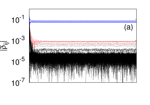
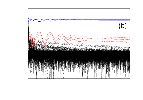
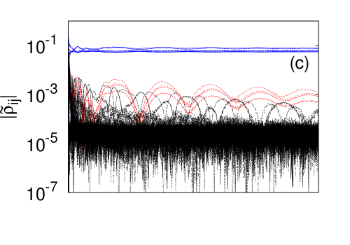
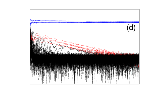
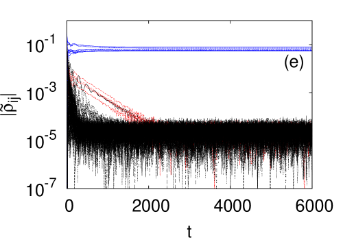
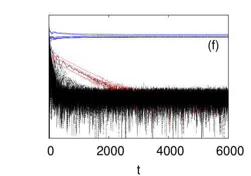
Figure 10: (Color online) Time evolution of the components $\widetilde{\rho}_{ij}$ of the reduced density matrix of the system with $N=26$ and $N_{S}=4$. The initial state is $UDUDY$. (a) Case II. Starting from case II, $1$ (b), $2$ (c), $4$ (d), $6$ (e) and $8$ (f) random bonds are introduced in $H_{E}$. Blue lines: diagonal components $|\widetilde{\rho}_{ii}|$; red lines: all $6$ slowly decaying components for $|\widetilde{\rho}_{ij}|$ for one random bond; black lines: all other $114$ off-diagonal components $|\widetilde{\rho}_{ij}|$.

For understanding the behavior of $\sigma(t)$ in case II with randomness, we investigate the individual components of the reduced density matrix $\widetilde{\rho}$ for the ring system. We study the addition of one, two, up to eight randomly replaced bonds in the environment. Recall that once the position for one random bond is chosen, this is also one of the random bonds when there are two or more random bonds. Similarly, the locations of the random positions for a large number of random bonds include the same positions and strengths as for a smaller number of random bonds. Furthermore, the same initial state “$Y$” of the environment is chosen for all simulations. We studied the effect of varying the positions of the randomly chosen bonds and of different initial states “$Y$” for the environment for a couple systems and did not find significant changes in our observations.

Figure 10 presents the results of the time evolution of the absolute value $|\widetilde{\rho}_{ij}|$ of the individual components of the reduced density matrix. For completeness we show both the diagonal components and the off-diagonal components. Figure 10 shows that most of the $120$ off-diagonal components quickly relax to a small value ($114$ black lines in Fig. 10 (b)-(e)). The slowest decaying $|\widetilde{\rho}_{ij}|$ are plotted in red. There are six such components. In the steady state all $|\widetilde{\rho}_{ij}|$ oscillate but have nearly the same time-averaged value, in agreement with the mean-field-type argument given in Appendix B. Thus, only a few $|\widetilde{\rho}_{ij}|$ are responsible for the lack of scaling of $\sigma$ in case II when starting from the initial state $UDUDY$, and also for the long times required to approach the predicted value of Eq. (10) of $\sigma(t)$ in the case that there are one or two random bonds.

VI Conclusions and Discussion

The main theoretical result of the current paper is Eq. (10) for the decoherence of a quantum system $S$ coupled to a quantum environment $E$. For studying decoherence we examine $\sigma(t)$, which is the square root of the sum of all the off-diagonal elements of the reduced density matrix $\widetilde{\rho}$ for $S$ in the basis that diagonalizes the Hamiltonian $H_{S}$ of the system $S$. We find (see also Eq. (10)) that

$$\sigma\approx\frac{1}{\sqrt{2D_{E}}}\left(1-\frac{1}{2D_{S}}\right),$$ (14)

where the reduced density matrix $\widetilde{\rho}$ for $S$ is a $D_{S}\times D_{S}$ matrix while the density matrix of the whole system $S+E$ is a $D\times D$ matrix with $D=D_{S}D_{E}$. Thus $D_{E}$ does not have to be very large in order for the predicted scaling to hold, in particular the scaling requires $D_{E}\gg 1\gg D_{S}^{-1}$. In addition the scaling requires that $S+E$ is driven from an initial wave function toward a steady state which is well described by a state which we called “$X$”.

We have performed large-scale real-time simulations of the time-dependent Schrödinger equation for $N_{S}$ spins in the system and $N_{E}$ spins in the environment. We have simulated spin-$1/2$ systems with $N=N_{S}+N_{E}$ up to $N=34$, all with $N_{S}=4$. Starting from a state “$X$” for $S+E$ the simulations agree very well with the scaling prediction Eq. (14), as shown in Fig. 2. In Appendix C we demonstrate that in this case not only the off-diagonal elements of $\widetilde{\rho}$ obey a scaling relation but also its diagonal elements obey a scaling relation, although a different one.

Therefore as long as the dynamics drives the initial state to a state “$Z$” which has similar properties as “$X$” the scaling relation Eq. (14) should hold. The next step is to examine under what conditions our test quantum model is driven to the state “$Z$”, and study the time scale needed to relax from an initial state to the state “$Z$”. For the one-dimensional quantum spin-$1/2$ ring we find that homogeneous couplings do not lead to an evolution to the state “$Z$” (Fig. 4), and hence the scaling as $1/\sqrt{D_{E}}$ is not observed. This conclusion is not modified if some randomly chosen homogeneous small world bonds are added (Fig. 8). Also systems with random couplings and random small world bonds between system and environment spins such that the maximum number of system spins that interact with one environment spin is two or larger do not evolve to a state “Z” (Fig. 7c). In this case, the environment requires a more complex connectivity than the simple one-dimensional one in order to observe the scaling as $1/\sqrt{D_{E}}$ (Fig. 7d). Therefore, although we find that some randomness in the interaction strengths in $E$ or between $S$ and $E$ the dynamics is very important to drive the whole system toward the state “$Z$”, as seen in Figs. 3, 5, 7a,b, and 9 it is not always sufficient. Moreover it may take a long time to evolve toward the state “$Z$” if there is only a little randomness (Fig. 9) or if the environment $E$ is large (the $N=34$ results of Fig. 3). The long time that may be required to approach the state “$Z$” is due to only a few off-diagonal elements of $\widetilde{\rho}$, as seen in Fig. 10. We find that the approach to the state “$Z$” can be sped up by adding randomness to $E$ (Figs. 9 and 10).

What do our results say about the approach to the quantum canonical ensemble? The canonical ensemble is given by the diagonal elements of the reduced density matrix $\widetilde{\rho}$ if the off-diagonal elements (as measured by $\sigma(t)$) can be neglected Kubo et al. (1985); Jin et al. (2010). As long as $E$ has a finite Hilbert space $D_{E}$ our scaling results can be used to argue that in a strict sense, the system will not be in the canonical state unless $D_{E}\rightarrow\infty$. However, if the canonical distribution is to be a good approximation for some temperatures $T$ up to some chosen maximum energy $E_{\rm hold}>0$, then this requires that $\exp\left(-E_{\rm hold}/k_{B}T\right)\gg\sigma$ which gives for our spin-$1/2$ system $k_{B}T\gg 2E_{\rm hold}/\left[N_{E}\ln(2)\right]$. For this argument to hold in the canonical distribution the energies are taken to be positive values above the ground state energy. This lack of thermalization at low temperatures for small systems is supported by simulations in Ref. Jin et al. (2010).

What do our results say about trying to prolong the time to decoherence in order to build practical quantum encryption or quantum computational devices? The important thing is to ensure that the system is not driven toward the state “$Z$”, or at least that it takes a very long time to approach the state “$Z$”. This can be achieved by changing the Hamiltonian of the system, $H=H_{S}+H_{E}+H_{SE}$, such that it has very small randomness particularly in the coupling between the system and the environment, $H_{SE}$. Alternatively extrapolating from Fig. 10 if one can devise an experimental procedure, for example a time-dependent procedure, to keep even a few of the off-diagonal elements of $\widetilde{\rho}$ large then the scaling prediction Eq. (14) for the decoherence can be avoided, at least for reasonable timescales.

The scaling of Eq. (14) can be contrasted with the predicted scaling of the Hilbert space variant of a whole system which should be proportional to $(D+1)^{-1}$ for the expectation value of a local operator Bartsch and Gemmer (2009). The results of the current research are also relevant for methodologies for measuring finite-temperature dynamical correlations Long et al. (2003) without performing the complete TDSE evolution of the whole system.

We leave as future work the coupling between a system $S$ composed of spin-$1/2$ objects (qubits) and an environment $E$ composed of harmonic oscillators. In particular, we have recently been able to build on exact calculations of a single spin coupled to specific types of spin environment Rao et al. (2008) to devise an algorithm that does not have computer memory constraints limited by the size of $D_{E}$ Novotny et al. (2012a, b). We are working to extend this algorithm to other types of environment and for more than one spin in the system $S$.

Appendix A Scaling without an environment

For comparison of the scaling of $\sigma(t)$ for the cases with and without an environment, we derive the scaling for the case of no environment. In the energy basis $\left|i\right\rangle$ of the (system, which is now the whole system) Hamiltonian $H$, the density matrix has elements

$$\rho_{ij}(t)=c_{i}(t)c_{j}^{\dagger}(t)\>.$$ (15)

We use from Ref. Hams and De Raedt (2000) the equations (A.12) and (A.23). The expectation value is

$$E\left(2\sigma^{2}\right) = E\left(\sum_{i=1}^{D_{S}}\sum_{j\neq i}^{D_{S}}\left|c_{i}(t)c_{j}(t)\right|^{2}\right)=\sum_{i=1}^{D_{S}}\sum_{j\neq i}^{D_{S}}E\left(\left|c_{i}(t)c_{j}(t)\right|^{2}\right)$$ (16)

$$= D_{S}\left(D_{S}-1\right)E\left(\left|c_{i}(t)\right|^{2}\left|c_{j}(t)\right|^{2}\right)=1-\frac{2}{D_{S}+1}\>=\>\frac{D_{S}-1}{D_{S}+1}\>.$$ (17)

The final scaling result for the quantity $\sigma$ that we measure is

$$\sigma\approx\frac{1}{\sqrt{2}}\sqrt{E\left(2\sigma^{2}\right)}=\frac{1}{\sqrt{2}}\sqrt{\frac{D_{S}-1}{D_{S}+1}}=\frac{1}{\sqrt{2}}-\frac{1}{\sqrt{2}D_{S}}+\frac{1}{2\sqrt{2}D_{S}^{2}}-\frac{1}{2\sqrt{2}D_{S}^{3}}+\frac{3}{8\sqrt{2}D_{S}^{4}}+\cdots\>.$$ (18)

Therefore without an environment, $\sigma$ approaches a constant as the size of the system (which is the whole system) grows. This also means that for the state “$X$”, if all off-diagonal elements are the same they will have a size of $\left|\rho_{ij}(t)\right|^{2}=1/D_{S}\left(D_{S}-1\right)\sim 1/D_{S}^{2}$ while if all the diagonal elements are equal (corresponding to infinite temperature) $\left|\rho_{ii}(t)\right|^{2}=1/D_{S}$ since ${\rm Tr}~{}\rho(t)=1$. We have performed simulations (results not shown) to ensure that for the case without an environment $\sigma$ obeys the scaling relation of Eq. (18) and it does.

Appendix B Mean-field-like reduced density matrix

We make a connection between $\sigma$ and the quantum purity ${\cal P}={\rm Tr}\left(\left(\hat{\rho}\right)^{2}\right)$. We assume a ‘mean-field-type’ structure for the reduced density matrix, namely we assume that all off-diagonal elements have the same size, $\epsilon$. In our simulations we find that in the energy basis the imaginary part of the off-diagonal elements are very small, which validates our hypothesis. However, the signs of the real part of the off-diagonal elements are not the same, which brings into question our ‘mean-field-like’ assumption. Nevertheless, we make the assumption that

$$\epsilon=\sqrt{\frac{2\sigma^{2}}{D_{S}\left(D_{S}-1\right)}}\>.$$ (19)

We introduce the matrix ${\bf J}$ with all its elements having the value $1$, the matrix ${\bf D}$ which is the diagonal matrix composed of the diagonal elements of ${\hat{\rho}}$, and the identity matrix ${\bf I}$. Note that ${\bf J}^{2}=D_{S}{\bf J}$. The ‘mean-field-type’ assumption then reads

$${\hat{\rho}}={\bf D}+\epsilon{\bf J}-\epsilon{\bf I},$$ (20)

which as seen from the graphs in Fig. 10 should be a reasonable assumption in the steady state regime. We will use the relationships

$${\rm Tr}\left({\bf D}\right) = 1,$$ (21)

$${\rm Tr}\left({\bf D}^{2}\right) \leq 1,$$ (22)

$${\rm Tr}\left({\bf I}\right) = {\rm Tr}\left({\bf J}\right)=D_{S},$$ (23)

$${\rm Tr}\left({\bf D}{\bf J}\right) = {\rm Tr}\left({\bf J}{\bf D}\right)=1,$$ (24)

$${\rm Tr}\left({\bf J}^{2}\right) = D_{S}^{2},$$ (25)

with the first relationship being a consequence of the trace of a density matrix being equal to unity. Then one has that

$${\cal P} = {\rm Tr}\left({\hat{\rho}}^{2}\right)$$ (26)

$$= {\rm Tr}\left(\left({\bf D}+\epsilon{\bf J}-\epsilon{\bf I}\right)^{2}\right)$$ (27)

$$= {\rm Tr}\left({\bf D}^{2}-2\epsilon{\bf D}+\epsilon^{2}{\bf I}+\epsilon{\bf D}{\bf J}+\epsilon{\bf J}{\bf D}-2\epsilon^{2}{\bf J}+\epsilon^{2}{\bf J}^{2}\right)$$ (28)

$$= {\rm Tr}\left({\bf D}^{2}\right)+2\sigma^{2}$$ (29)

$$= {\rm Tr}\left({\bf D}^{2}\right)+\frac{1-\frac{1}{D_{S}}}{D_{E}+\frac{1}{D_{S}}}$$ (30)

$$= {\rm Tr}\left({\bf D}^{2}\right)$$ (32)

$$+\frac{1}{D_{E}}\left(1-\frac{1}{D_{S}}-\frac{1}{D_{E}D_{S}}+\frac{1}{D_{E}D_{S}^{2}}+\cdots\right)\>.$$

In the canonical ensemble the diagonal elements of the reduced density matrix are related to the terms in the canonical partition function, in particular ${\hat{\rho}}_{ii}=e^{-\beta E_{i}}/Z$ Yuan et al. (2009); Jin et al. (2010). Therefore we have a connection between the quantum purity ${\cal P}$ and how close the system is to a canonical ensemble. In the steady state this difference is of the order of $1/D_{E}$.

With the same ‘mean-field-like’ assumption for ${\hat{\rho}}$ in the steady state one can look at corrections to the von Neumann entropy of the system, ${\cal S}=-{\rm Tr}\left({\hat{\rho}}{\rm ln}{\hat{\rho}}\right)$. However, we do not find the final result too enlightening.

Appendix C Diagonal elements of the reduced density matrix

In the main text, we investigated the scaling property of the off-diagonal elements of the reduced density matrix of a system coupled to an environment. For being complete in the contents, we present some numerical and analytical results concerning the diagonal elements.

In general, based on the fact that the system decoheres, i.e. the off-diagonal elements of the reduced density matrix approach zero, we expect that the diagonal elements take (approach to) the form of the canonical distribution $\exp(-\beta E_{i})$ where $\beta=1/k_{B}T$ with $T$ denoting the temperature and $k_{B}$ Boltzmann’s constant, which is taken to be one in this paper, and where $E_{i}$’s denote the eigenvalues of $H_{S}$ Yuan et al. (2009); Jin et al. (2010). The difference between the diagonal elements $\widetilde{\rho}_{ii}\left(t\right)$ and the canonical distribution is conveniently characterized by

$$\delta(t)=\sqrt{\sum_{i=1}^{D_{S}}\left(\widetilde{\rho}_{ii}(t)-\left.{e^{-b(t)E_{i}}}\right/{\sum_{i=1}^{D_{S}}e^{-b\left(t\right)E_{i}}}\right)^{2}},$$ (33)

with a fitting inverse temperature

$$b(t)=\frac{\sum_{i<j,E_{i}\neq E_{j}}[\ln\widetilde{\rho}_{ii}(t)-\ln\widetilde{\rho}_{jj}(t)]/({E_{j}-E_{i}})}{\sum_{i<j,E_{i}\neq E_{j}}1}.$$ (34)

If the system relaxes to its canonical distribution both $\delta(t)$ and $\sigma(t)$ are expected to vanish, $b(t)$ converging to the effective inverse temperature $b$.

Figure 11: Simulation results for the time-averaged value $\bar{\delta}$ of $\delta(t)$ (see Eq. (33)) for case I (bullets) and case II (squares) for different sizes $N$ of the whole system. The initial state of the whole system is “$X$” (see text). The dotted line is $1/\sqrt{2^{N}}$.

The numerical simulations of which we present the results correspond to those used to make Fig. 2. The initial state for those simulations is “$X$”. We analyze the diagonal elements, instead of the off-diagonal elements, of the reduced density matrix and calculate the quantity $\delta(t)$. In Fig. 11, we present the time-averaged value $\overline{\delta}$ of $\delta(t)$ for each system size. It is interesting to see that the quantity $\overline{\delta}$ also has a kind of scaling property. As the whole system size $N$ increases, $\overline{\delta}$ decreases as $1/\sqrt{D}$, where $D=2^{N}$.

In fact the fitting inverse temperature $b(t)$ is very close to zero for reasonablely large $N_{E}$ (data not shown). The canonical distribution of $S$ at $b=0$ is represented by a diagonal density matrix with elements $1/D_{S}$, where $D_{S}=2^{N_{S}}$. Then, we are able to derive the scaling property for $\delta$ as we did to obtain Eq. (7). The expectation value of $\delta$ is given by

$$E\left(\delta^{2}\right) = E\left(\sum_{i=1}^{D_{S}}\left|\sum_{p=1}^{D_{E}}C_{i,p}^{*}C_{i,p}-\frac{1}{D_{S}}\right|^{2}\right)=\sum_{i=1}^{D_{S}}\>\sum_{p=1,p^{\prime}=1}^{D_{E}}E\left(\left|C_{i,p}\right|^{2}\left|C_{i,p^{\prime}}\right|^{2}\right)-\frac{1}{D_{S}}$$ (35)

$$= \sum_{i=1}^{D_{S}}\>\sum_{p=1,p^{\prime}=1}^{D_{E}}\left(\left(1-\delta_{p,p^{\prime}}\right)E\left(\left|C_{i,p}\right|^{2}\left|C_{i,p^{\prime}}\right|^{2}\right)+\delta_{p,p^{\prime}}E\left(\left|C_{i,p}\right|^{4}\right)\right)-\frac{1}{D_{S}}$$ (36)

$$= \sum_{i=1}^{D_{S}}\>\sum_{p=1,p^{\prime}=1}^{D_{E}}\left(\left(1-\delta_{p,p^{\prime}}\right)\frac{1}{D(D+1)}+\delta_{p,p^{\prime}}\frac{2}{D(D+1)}\right)-\frac{1}{D_{S}}$$ (37)

$$= \frac{D_{E}+1}{D+1}-\frac{1}{D_{S}}=\frac{D_{S}-1}{D_{S}}\frac{1}{D+1}\>.$$ (38)

From Eq. (35), we have $\delta\approx 1/\sqrt{D}$ for $D_{S}>1$ and $D_{E}\gg 1$. Therefore, if the size of the environment goes to infinity with the final state being the state “$X$”, the diagonal elements of the reduced density matrix of the system approach $1/D_{S}$.

References

- Kubo et al. (1985) R. Kubo, M. Toda, and N. Hashitsume, Statistical physics II: Nonequilibrium statistical mechanics (Springer-Verlag, New York, 1985).
- Nielsen and Chuang (2000) M. Nielsen and I. Chuang, Quantum Computation and Quantum Information (Cambridge University Press, Cambridge, 2000).
- Yukalov (2011) V. Yukalov, Laser Phys. Lett. 8, 485 (2011).
- von Neumann (1929) J. von Neumann, Z. Phys. 57, 30 (1929).
- Peres (1984) A. Peres, Phys. Rev. A 30, 504 (1984).
- Deutsch (1991) J. Deutsch, Phys. Rev. A 43, 2046 (1991).
- Tasaki (1998) H. Tasaki, Phys. Rev. Lett. 80, 1373 (1998).
- Goldstein et al. (2006) S. Goldstein, J. L. Lebowitz, R. Tumulka, and N. Zanghì, Phys. Rev. Lett. 96, 050403 (2006).
- Popescu et al. (2006) S. Popescu, A. J. Short, and A. Winter, Nature Phys. 2, 754 (2006).
- Reimann (2007) P. Reimann, Phys. Rev. Lett. 99, 160404 (2007).
- Linden et al. (2009) N. Linden, S. Popescu, A. J. Short, and A. Winter, Phys. Rev. E 79, 061103 (2009).
- Short (2011) A. Short, New. J. Phys. 13, 053009 (2011).
- Reimann (2010) P. Reimann, New. J. Phys. 12, 055027 (2010).
- Ponomarev et al. (2011) A. Ponomarev, S. Denisov, and P. Hänggi, Phys. Rev. Lett. 106, 010405 (2011).
- Ponomarev et al. (2012) A. Ponomarev, S. Denisov, P. Hänggi, and J. Gemmer, Europhys. Lett. 98, 40011 (2012).
- Yuan et al. (2009) S. Yuan, M. Katsnelson, and H. De Raedt, J. Phys. Soc. Jpn. 78, 094003 (2009).
- Jin et al. (2010) F. Jin, S. Yuan, H. De Raedt, K. Michielsen, and S. Miyashita, J. Phys. Soc. Jpn. 79, 074401 (2010).
- De Raedt and Michielsen (2006) H. De Raedt and K. Michielsen, in Handbook of Theoretical and Computational Nanotechnology, edited by M. Rieth and W. Schommers (American Scientific Publishers, Los Angeles, 2006) pp. 2 – 48.
- Hams and De Raedt (2000) A. Hams and H. De Raedt, Phys. Rev. E 62, 4365 (2000).
- von Neumann (1955) J. von Neumann, Mathematical Foundations of Quantum Mechanics (Princeton University Press, Princeton, 1955).
- Ballentine (2003) L. E. Ballentine, Quantum Mechanics: A Modern Development (World Scientific, Singapore, 2003).
- Tal-Ezer and Kosloff (1984) H. Tal-Ezer and R. Kosloff, J. Chem. Phys. 81, 3967 (1984).
- Leforestier et al. (1991) C. Leforestier, R. Bisseling, C. Cerjan, M. Feit, R.Friesner, A. Guldberg, A. Hammerich, G. Jolicard, W. Karrlein, H.-D. Meyer, N. Lipkin, O. Roncero, and R. Kosloff, J. Comp. Phys. 94, 59 (1991).
- Iitaka et al. (1997) T. Iitaka, S. Nomura, H. Hirayama, X. Zhao, Y. Aoyagi, and T. Sugano, Phys. Rev. E 56, 1222 (1997).
- Dobrovitski and De Raedt (2003) V. Dobrovitski and H. De Raedt, Phys. Rev. E 67, 056702 (2003).
- De Raedt et al. (2007) K. De Raedt, K. Michielsen, H. De Raedt, B. Trieu, G. Arnold, M. Richter, T. Lippert, H. Watanabe, and N. Ito, Comp. Phys. Comm. 176, 121 (2007).
- Gemmer and Michel (2006) J. Gemmer and M. Michel, Eur. Phys. J. B 53, 517 (2006).
- Yuan et al. (2006) S. Yuan, M. Katsnelson, and H. De Raedt, JETP Lett. 84, 99 (2006).
- Yuan (2011) S. Yuan, J. Comput. Theor. Nanoscience 8, 889 (2011).
- Brox et al. (2012) H. Brox, J. Bergli, and Y. M. Galperin, Phys. Rev. A 85, 052117 (2012).
- Bartsch and Gemmer (2009) C. Bartsch and J. Gemmer, Phys. Rev. Lett 102, 110403 (2009).
- Long et al. (2003) M. W. Long, P. Prelovšek, S. El Shawish, J. Karadamoglou, and X. Zotos, Phys. Rev. B 68, 235106 (2003).
- Rao et al. (2008) D. D. B. Rao, H. Kohler, and F. Sols, New J. Phys. 10, 115017 (2008).
- Novotny et al. (2012a) M. A. Novotny, M. Guerra, H. De Raedt, K. Michielsen, and F. Jin, J. Phys.: Conf. Ser. 402, 012019 (2012a).
- Novotny et al. (2012b) M. A. Novotny, M. Guerra, H. De Raedt, K. Michielsen, and F. Jin, Physics Procedia 34, 90 (2012b).