Relative velocity of dark matter and barions in clusters of galaxies and measurements of their peculiar velocities

Abstract

The increasing sensitivity of current experiments, which nowadays routinely measure the thermal SZ effect within galaxy clusters, provide the hope that peculiar velocities of individual clusters of galaxies will be measured rather soon using the kinematic SZ effect. Also next generation of X-ray telescopes with microcalorimeters, promise first detections of the motion of the intra cluster medium (ICM) within clusters. We used a large set of cosmological, hydrodynamical simulations, which cover very large cosmological volume, hosting a large number of rich clusters of galaxies, as well as moderate volumes where the internal structures of individual galaxy clusters can be resolved with very high resolution to investigate, how the presence of baryons and their associated physical processes like cooling and star-formation are affecting the systematic difference between mass averaged velocities of dark matter and the ICM inside a cluster. We, for the first time, quantify the peculiar motion of galaxy clusters as function of the large scale environment. We also demonstrate that especially in very massive systems, the relative velocity of the ICM compared to the cluster peculiar velocity add significant scatter onto the inferred peculiar velocity, especially when measurements are limited to the central regions of the cluster. Depending on the aperture used, this scatter varies between 50% and 20%, when going from the core (e.g. ten percent of the virial radius) to the full cluster (e.g. the virial radius).

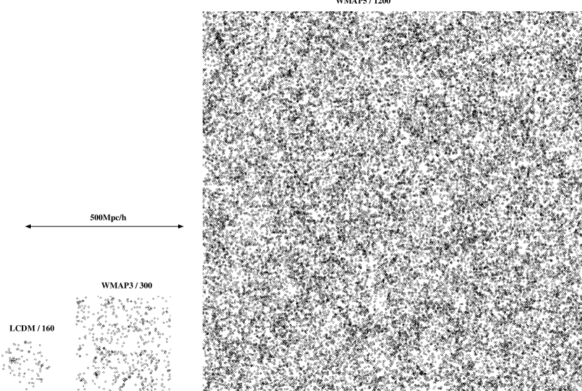
Figure 1: Visualization of the 3 different simulations used. Shown are the position of all galaxy clusters with masses above $10^{14}M_{\odot}/h$.

1 Introduction

The increasing sensitivity of the South Pole Telescope, ACT, PLANCK, MUSTANG, CARMA, AMIBA, AMI and several other CMB experiments provide the hope that peculiar velocities of individual clusters of galaxies will be measured rather soon using the kinematic effect (Sunyaev & Zeldovich, 1980). Also next generation of X-ray telescopes with microcalorimeters, like the soon coming Astro-H mission or the planned Athena or SMART-X missions will be able to measure the kinematic of the intra cluster medium (ICM) with so far unaccomplished precision. In fact, recently the Atacama Telescope Team announced their first detection of the kinematic SZ (kSZ) effect due to the relative motion of the groups of galaxies (Hand et al., 2012). Thereby, measuring the kinematic SZ effect opens a unique and direct method of measuring the peculiar velocities of the the hot ICM in clusters and groups of galaxies relative to CMB monopole and if associated to the peculiar velocity of clusters in general probe for the first time an so far unexplored prediction of our cosmological model (for example recently Keisler & Schmidt (2012) considered the measurement of the such signal to constrain models of modified gravity). More precisely, kSZ measurements are able to provide the value of the radial component of the ICM peculiar velocity $v_{\mathrm{pec,ICM}}^{r}$ relative to the local CMB monopole at the position of the cluster of galaxies,

$$\frac{\Delta T_{\mathrm{CMB}}}{T_{\mathrm{CMB}}}=-\frac{\sigma_{t}}{c}\int n_{e}v_{\mathrm{pec,ICM}}^{r}\mathrm{d}r,$$ (1)

folded with the local electron density $n_{e}$ which needs to be additionally inferred from X-ray observations; here $\sigma_{T}$ and $c$ denote the Thomson cross-section and the speed of light, respectively. Microcalorimeters on-board of future X-ray satellites will be able to provide the redshift of the gas radiating in the iron 6.7 and 6.9 keV lines. This redshift represents the sum of the Hubble recession velocity $v_{\mathrm{Hubble}}(z)$ and the radial component of peculiar velocity of the ICM within the cluster,

$$v_{\mathrm{X-ray}}=v_{\mathrm{Hubble}}(z)+v_{\mathrm{pec,ICM}}^{r}$$ (2)

At the same time, the broadening of the 6.7 keV line complex will give information about turbulence and bulk motions in ICM (see discussion in Inogamov & Sunyaev, 2003; Dolag et al., 2005). Therefore combining X-ray and kSZ measurements permit to separate the Hubble flow velocity and peculiar velocity of ICM. However, in galaxy clusters the situation is more complex, as the average radial peculiar velocities of ICM and the halo as a whole (including dark matter, ICM and mass in galaxies and field stars) can differ significantly. As a result an unavoidable systematic error will appear when the peculiar velocity of clusters of galaxies as a whole is inferred from observations.

It is well known that both ICM and dark matter in clusters of galaxies have large bulk motions due to merging of clusters of galaxies with other clusters or groups of galaxies, infall of fresh dark matter and ICM in the filaments (Frenk et al., 1999; Sunyaev et al., 2003) and activity of a black hole in the center of the dominant galaxies (Churazov et al., 2001). These motions often have velocities of order the sound speed of the ICM and thereby exceeding several times the expected peculiar velocity of the cluster as a whole. Observationally, such bulk motions can be seen by induced cold fronts or even shocks within the ICM (see Markevitch & Vikhlinin, 2007, for a review). Such cold fronts suggest that large regions of clusters (e.g. the whole core) can have systematic velocity offsets compared to the peculiar velocity of the galaxy cluster and therefore could significantly affect the kSZ measurements (Diego et al., 2003). These velocity offsets are also reflected in the observed offset between X-ray and weak lensing centers (Planck Collaboration, 2012) as well as the displacement of the central galaxy from the mass center of the galaxy cluster (Zitrin et al., 2012). From X-ray observations, current measurements of the line broadening so far give only upper limits on the turbulent motions within the ICM (Sanders et al., 2011; Bulbul et al., 2012), however interpretation of the pressure fluctuations observed in the Coma galaxy clusters indicate turbulent velocities at a level of 10% of the sound speed (Schuecker et al., 2004). It has been recently confirmed that the observed fluctuations in the X-ray surface brightness of Coma would be compatible with turbulent velocities of several hundreds of km/s (Churazov et al., 2012). Additionally, Simionescu et al. (2012) recently presented the evidence for the presence of bulk motions far beyond the core regions in the Perseus cluster based on measured X-ray surface brightness features.

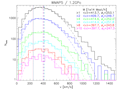
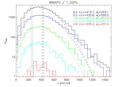
Figure 2: Histogram of the peculiar motion of galaxy clusters from the large cosmological box WMAP5 / 1200. Shown in the left panel are the histograms for clusters above $10^{14}$, $2\times 10^{14}$, $4\times 10^{14}$, $6\times 10^{14}$, $8\times 10^{14}$ and $10^{15}$ $M_{\odot}/h$ whereas the right panel shows the histograms for clusters above $10^{14}$ $M_{\odot}/h$ for at redshift $z=2$, $z=1.5$, $z=1$, $z=0.5$ and $z=0$. Dashed vertical line marks the median velocity for which values are also quoted in the legends of the panels. The dashed line following the histograms is the best fit Maxwell distribution, whereas the vertical dotted line marks the standard deviation $\sigma_{v}$, for which values are also quoted in the legends of the panels.

Such large bulk motions motions are expected from cosmological simulations (Sunyaev et al., 2003; Inogamov & Sunyaev, 2003) and will drive turbulence within the ICM (Bryan & Norman, 1998; Rasia et al., 2004; Dolag et al., 2005; Vazza et al., 2006, 2009, 2011; Iapichino & Niemeyer, 2008; Paul et al., 2011). Additionally, it has been also shown that gravitational perturbations alone (as expected within the cosmological environment of clusters) can by them self already induce significant motions within the core of clusters (e.g. Ascasibar & Markevitch, 2006; Roediger et al., 2011; ZuHone et al., 2010). Therefore kinematic effect is expected to strongly vary between different regions of the cluster. However, using non radiative, cosmological simulations, Nagai et al. (2003) concluded that the effect of these ICM motions in galaxy clusters is rather mild, adding only 50-100 km/s scatter to the observed kSZ signal. Using clusters extracted from a cosmological simulation which includes the effect of cooling and star-formation, Diaferio et al. (2005) find a 10% to 20% effect of the internal motion on the measured peculiar velocity. Additional, they found that the bias between the mass weighted temperature within the cluster and the X-ray measured temperature can increase this error significantly.

Using numerical simulations of very large cosmological volume, hosting a large number of rich clusters of galaxies we will study the systematic difference between mass averaged velocities of dark matter and the ICM inside galaxy clusters. Therefor we will use both, dark matter only simulations as well as simulations which are including baryons and their associated physical processes (like cooling and star-formation) to study their influence on the internal dynamics of galaxy clusters. We will thereby demonstrate in detail that this relative velocity between the observational signal of the hot ICM and the dark matter within massive clusters of galaxies is significantly larger than inferred previously and can introduce an approximately 30% systematic error to the peculiar velocity determination of massive systems.

We will discuss several independent ways to measure this relative velocity using X-ray instruments with micro-calorimeters as well as observations of the imprint of the ICM onto the CMB at radio wavelength, with both should soon become powerful instruments to measurements of the bulk motions and turbulence inside clusters of galaxies.

The paper is structured as follows: Section 2 describes the hydrodynamic simulations used in this paper. Section 3 and 4 generally summarize the peculiar velocity of galaxy clusters, the influence of baryons and how it is traced by by different constituents of the cluster. Section 5 the discusses large scale bulk motions which are present within clusters and how they differ in respect to the peculiar velocity of the whole cluster. In Section 6 we demonstrate the relative importance of these bulk motions to the observational available signal, where especially in sub-chapter 6.2 we discuss the different distributions of the bulk velocities of dark matter, intra cluster gas and light, and galaxies within spherical sub-shells at different cluster centric distances as present in massive clusters. In section 7 we show the application to the pairwise velocity signal before we summarize our findings in section 8.

2 Simulations

The results presented in this paper have been obtained using three different simulations capturing a wide range in mass and resolution. The largest simulations WMAP5 / 1200 captures a large enough volume to allow highly significant statistic of peculiar motions of clusters and super clusters and also allows to explore massive clusters at redshift ranges above z=1. In the medium simulation WMAP3 / 300 , clusters are resolved enough to allow to study the systematic differences in the peculiar motion of the whole clusters and bulk motions of different parts of the embedded ICM. In the highest resolution simulation LCDM / 160 gas physics and star-formation is resolved enough to allow a de-composition of the stellar component and to distinguish the motion of dark matter in respect to the stars within the central cD, the stars within individual galaxies as well as the stars within the so called intra cluster light component. Figure 1 gives a visual impression of the different simulations. Shown are the positions of all clusters above a mass of $10^{14}M_{\odot}/h$ within the individual simulations. If not mentioned otherwise, the simulations where performed with the GADGET-3 code (Springel et al., 2001; Springel, 2005), which makes use of the entropy-conserving formulation of SPH (Springel & Hernquist, 2002). These hydrodynamical simulations include radiative cooling, heating by a uniform redshift–dependent UV background (Haardt & Madau, 1996), and a treatment of star formation and feedback processes. The latter is based on a sub-resolution model for the multiphase structure of the interstellar medium (Springel & Hernquist, 2003) with parameters which have been fixed to get a wind velocity of $\approx 350$ km/s.

2.1 LCDM / 160

The highest resolution simulation used reuses the final output of a cosmological hydrodynamical simulation of the local universe. Our initial conditions are similar to those adopted by Mathis et al. (2002) in their study (based on a pure N-body simulation) of structure formation in the local universe. The galaxy distribution in the IRAS 1.2-Jy galaxy survey is first Gaussian smoothed on a scale of 7 Mpc and then linearly evolved back in time up to $z=50$ following the method proposed by Kolatt et al. (1996). The resulting field is then used as a Gaussian constraint (Hoffman & Ribak, 1991) for an otherwise random realization of a flat $\Lambda$CDM model, for which we assume a present matter density parameter $\Omega_{\mathrm{0m}}=0.3$, a Hubble constant $H_{0}=70$ km/s/Mpc and a r.m.s. density fluctuation $\sigma_{8}=0.9$. The volume that is constrained by the observational data covers a sphere of radius $\sim 80$ Mpc/h, centered on the Milky Way. This region is sampled with more than 50 million high-resolution dark matter particles and is embedded in a periodic box of $\sim 240$ Mpc/h on a side. The region outside the constrained volume is filled with nearly 7 million low-resolution dark matter particles, allowing a good coverage of long-range gravitational tidal forces.

Unlike in the original simulation made by Mathis et al. (2002), where only the dark matter component is present, here we followed also the gas and stellar component. For this reason we extended the initial conditions by splitting the original high-resolution dark matter particles into gas and dark matter particles having masses of $m_{\mathrm{gas}}\approx 0.48\times 10^{9}\;M_{\odot}/h$ and $m_{\mathrm{dm}}\approx 3.1\times 10^{9}\;M_{\odot}/h$, respectively; this corresponds to a cosmological baryon fraction of 13 per cent. The total number of particles within the simulation is then slightly more than 108 million and the most massive clusters is resolved by almost one million particles. The gravitational force resolution (i.e. the comoving softening length) of the simulation has been fixed to be 7 kpc/h (Plummer-equivalent), fixed in physical units from z=0 to z=5 and then kept fixed in comoving units at higher redshift.

In addition, this simulation follows the pattern of metal production from the past history of cosmic star formation (Tornatore et al., 2004, 2007). This is done by computing the contributions from both Type-II and Type-Ia supernovae and energy feedback and metals are released gradually in time, accordingly to the appropriate lifetimes of the different stellar populations. This treatment also includes, in a self-consistent way, the dependence of the gas cooling on the local metalicity. The feedback scheme assumes a Salpeter IMF (Salpeter, 1955), and its parameters have been fixed to get a wind velocity of $\approx 480$ km/s.

More detailed information regarding this simulation and the technique to distinguish between the satellite galaxies, the cD and the ICL component can be found in Dolag et al. 2010.

2.2 WMAP3 / 300

As medium size cosmological simulation we used a cosmological box of size $(300{\rm{Mpc}}/h)^{3}$, resolved with $(768)^{3}$ dark matter particles with a mass of $m_{\mathrm{dm}}\approx 3.7\times 10^{9}{\rm{M_{\odot}}}h^{-1}$ and the same amount of gas particles, having a mass of $m_{\mathrm{gas}}\approx 7.3\times 10^{8}{\rm{M_{\odot}}}\ h^{-1}$. Here we use the concordance $\Lambda$CDM model, adapted to the WMAP3 values (Spergel et al., 2007), which assumes a matter density of $\Omega_{\mathrm{0m}}=0.268$, a baryon density of $\Omega_{\mathrm{0b}}=0.044$, a Hubble parameter $h=0.704$, a power spectrum normalization of $\sigma_{8}=0.776$ and a spectral index of $n_{s}=0.947$. More information on this simulation can be found in De Boni et al. (2011, 2012) and Fedeli et al. (2012).

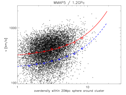
Figure 3: Dependence of the cluster peculiar motion on the large scale environment. Shown are the peculiar motions of all clusters above $2\times 10^{14}$ $M_{\odot}/h$ at z=0 from the large cosmological box WMAP5 / 1200 as function of the local over-density within 20 Mpc around each cluster. Clear to see that the median peculiar velocity (red diamonds, solid line) and similarly the best fit standard deviation $\sigma_{v}$ (blue diamonds, dashed line) rises by a factor of two between low density and high density environments.

2.3 WMAP5 / 1200

As large cosmological simulations we considered a box of (1200 Mpc/$h)^{3}$, resolved with $960^{3}$ dark matter particles with a mass of $m_{\rm{dm}}\approx 1.2\times 10^{11}h^{-1}\rm{M}_{\odot}$ and the same amount of gas particles, having a mass of $m_{\rm{gas}}\approx 2.4\times 10^{10}h^{-1}\rm{M}_{\odot}$. The gravitational force has a Plummer-equivalent softening length of $\epsilon_{l}=25h^{-1}$ kpc. This simulations assumes a ‘concordance’ $\Lambda$CDM model, where we fix the relevant parameters consistently with those derived from the analysis of the WMAP 5-year data (Komatsu et al., 2009): $\Omega_{\mathrm{m0}}=0.26$ for the matter density parameter, $\Omega_{\Lambda 0}=0.74$ for the $\Lambda$ contribution to the density parameter, $h=0.72$ for the Hubble parameter (in units of $100$ km s^-1 Mpc^-1). The initial power spectrum has a spectral index $n=0.96$ and is normalized in such a way that $\sigma_{8}=0.8$. More information on this simulation can be found in Grossi et al. (2009); Reid et al. (2010); Roncarelli et al. (2010), where the dark matter only counterpart of these simulations was used.

Figure 4: Distribution of the peculiar velocities of the clusters from figure 3 as function of the environmental over-density (solid lines) and the best fit to a Maxwell distribution (dashed lines).

2.4 Post processing

We are using SUBFIND (Springel et al., 2001; Dolag et al., 2009; Dolag et al., 2010) to define halo and sub-halo properties. SUBFIND thereby identifies substructures as locally overdense, gravitationally bound groups of particles. Starting with a halo identified through the Friends-of-Friends algorithm, a local density is estimated for each particle with adaptive kernel estimation using a prescribed number of smoothing neighbours. Starting from isolated density peaks, additional particles are added in sequence of decreasing density. Whenever a saddle point in the global density field is reached that connects two disjoint overdense regions, the smaller structure is treated as a substructure candidate, followed by merging the two regions. All substructure candidates are subjected to an iterative unbinding procedure with a tree-based calculation of the potential. The SUBFIND algorithm is discussed in full in (Springel et al., 2001) and its extension to dissipative hydrodynamical simulations that include star formation in Dolag et al. (2009). Based on a differences in the dynamics, the unbinding procedure for the central galaxy of each halo can be modified, which leads to a spatial separation of the two, dynamically well separated components into a cD and a diffuse stellar component (DSC). For details see Dolag et al. (2010).

The Mass and Radius of our clusters will refer to a spherical over-density according to a density contrast of 200 with respect to the mean density, which we associate with the viral properties. Synthetic maps of observables are produced using SMAC (Dolag et al., 2005). If not stated differently, we will call peculiar velocity the mean (and mass weighted among all constituents) velocity of a halo, averaged within the virial radius while we will generally refer to bulk motions if we speak about motions of certain components averaged over sub-regions within the cluster.

3 Cluster peculiar motions

The distribution of the overall peculiar motions of galaxy clusters reflect the large scale velocity field, which still probes the linear regime of structure formation. Therefore they are expected to follow a Maxwell distribution (Bahcall et al., 1994). In this section we discuss the cluster peculiar motion as extracted from the large, cosmological simulation (WMAP5 / 1200).

3.1 Mass and redshift dependence

For the current (low mass density) cosmology the typical (e.g. median) cluster peculiar motion is expected to of order of 400 km/s (Bahcall et al., 1994). Figure 2, shows the distribution of cluster peculiar velocities for different cut in cluster mass as well as for different redshifts. Independently on the actual cluster mass, or the redshift, the median peculiar velocities is $\approx 410$ km/s. They mainly follow an Maxwell distribution,

$$P(v_{\mathrm{pec}})=A_{0}v_{\mathrm{pec}}^{2}\mathrm{exp}\left(\frac{-v_{\mathrm{pec}}^{2}}{2\sigma_{v}^{2}}\right)$$ (3)

as expected (Bahcall et al., 1994), but with an excess at higher velocities (see next sub-section for a discussion of the origin of that excess). For a perfect, Maxwell distribution, the mean velocity $\left<v_{\mathrm{pec}}\right>$ is related to the standard deviation $\sigma_{v}$ by $\left<v_{\mathrm{pec}}\right>=\sqrt{8/\pi}\sigma_{v}$, which in this case gives a typical standard deviation of $\sigma_{v}\approx 250$ km/s.

3.2 Environment dependence of peculiar motions

To explain the origin of the excess of larger peculiar velocities we investigated the peculiar motion of the clusters as extracted from the large, cosmological simulation (WMAP5 / 1200) as function of the local over-density. Therefore, we selected all clusters above a mass limit of $2\times 10^{14}$ $M_{\odot}/h$ at z=0 and calculated the over-density of matter within a 20 Mpc sphere around each cluster. Figure 3 shows the distribution of the peculiar velocities as function of this large-scale over-density. Clear to see is the trend to have larger peculiar motions of clusters in higher density region, which boost the median cluster peculiar velocity by almost a factor of two in the high density regions. We also calculated the velocity distribution by binning the clusters by the over-density of the environment. In this case, the individual distributions follow very closely a Maxwell distribution without any excess at large velocities, as shown in figure 4, where the velocity distribution and the best fit Maxwell distribution are shown for the individual over-density bins. The best fit value for the standard deviation $\sigma_{v}$ (blue diamonds in figure 3) follows a functional form of

$$\sigma_{v}(\delta_{20\mathrm{Mpc}})=185\mathrm{km/s}\times\mathrm{exp}\left(\delta_{20\mathrm{Mpc}}/10\right)$$ (4)

which is shown as dashed line in figure 3. The mean peculiar velocity follow (as expected) exactly the same trend but multiplied by $\sqrt{8/\pi}$ as shown by the red diamonds and the solid line in figure 3.

The velocity difference of close pairs of galaxy clusters can also be used to boost the measurement of cluster peculiar motions (Diaferio et al., 2000). Figure 5 shows how the velocity difference between cluster pairs is boosted due to the merging process of large scale structure. Here, the distance $d$ is measured in units of the sum of the virial radii of the two clusters, meaning that $d=1$ on the x-axis means that the virial radii of the two clusters touch each other. It is worth to mention that only at larger distances (e.g. $d>3$) we find systems which actually move away from each other (blue stars) in figure 5, whereas close by systems always approach each other. This means that (as expected), violent relaxation for clusters is effective enough to do not allow a merging system to completely detach again (e.g. $d>1$). Of course, within the virial radius the merging process can produce gas rich sub-structures which might move in opposite directions, as observed in systems like the bullet cluster (Markevitch et al., 2004). The median velocity here can easily exceed 1000 km/s (red diamonds in figure 5) and therefore is 2.5 times larger than the median peculiar velocity of individual clusters. The solid line marks the simple functional form of

$$\left<v(d)\right>=270\mathrm{km/s}+1000\mathrm{km/s}\times d^{-1}$$ (5)

shown a solid (red) line in figure 5.

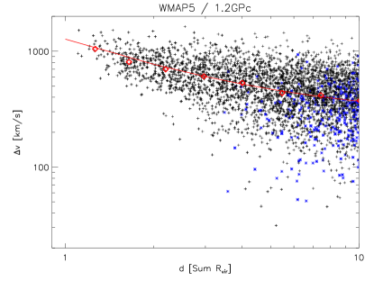
Figure 5: Dependence of the relative motions of clusters pairs on their distance. Shown are the all clusters above $2\times 10^{14}$ $M_{\odot}/h$ at z=0 from the large cosmological box WMAP5 / 1200. Crosses (black) are approaching systems, stars (blue) are systems which move away from each other. Clear to see that cluster pairs have an strong excess in their pairwise velocity compared to typical peculiar motions with even stronger signal for close pairs. Diamonds (red) are the median, pairwise velocity and the best power-law fit (line).

4 The influence of baryons

In this section we want to discuss the effect of baryonic material on the overall peculiar motions of galaxy clusters and especially the peculiar motions traced by the different components within galaxy clusters like dark matter, ICM and stars. As already mentioned, the distribution of the overall peculiar motions of galaxy clusters reflect the large scale velocity field, which still probes the linear regime of structure formation and therefore we do not expect the peculiar velocities to be effected by the presence of the baryonic component. This is demonstrated in detail in the Appendix A1, figure 17.

Although the cluster peculiar velocities (recap that those is the mass weighted mean over all constituents of the cluster) does not change significantly when baryonic physics is included it is interesting to see, if the mean velocity of the different individual constituents within the cluster differs. As we continue to look at mean values within the virial radius, we will still call them peculiar velocities. As we also want to include sub-structure, representing galaxies, we will switch here to the medium size cosmological box (WMAP3 / 300) as here we have good enough resolution to resolve at least 10 member galaxies in a $10^{14}$ $M_{\odot}/h$ halo and several hundred of member galaxies in the most massive systems. Figure 6 shows the peculiar velocity distribution as traced by the different components. There is not much difference between the distribution (and the median values) of the peculiar motion measured by the dark matter and the ICM component within the cluster. The ICM velocity match almost the peculiar velocity (within 1%). However, the peculiar velocity traced by the galaxies is slightly biased high (ca. 5%) when using the mass weighted mean and strongly biased (ca. 12%) when one calculate the peculiar velocity as the pure mean of the velocity of all galaxies. Obviously, when weighting the velocities of the individual galaxies by their (stellar) mass gives the central galaxy (which in this case additional inherits a large stellar component in form of the diffuse stellar component) a very large weight.

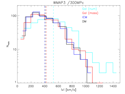
Figure 6: Histogram of the peculiar motion of galaxy clusters from the medium size cosmological box WMAP3 / 300 at $z=0$. Shown are the histograms for clusters above $10^{14}$ $M_{\odot}/h$ for the dark matter (black line), ICM (blue line) and galaxy component (red line for mass weighted, light blue line for number weighed).

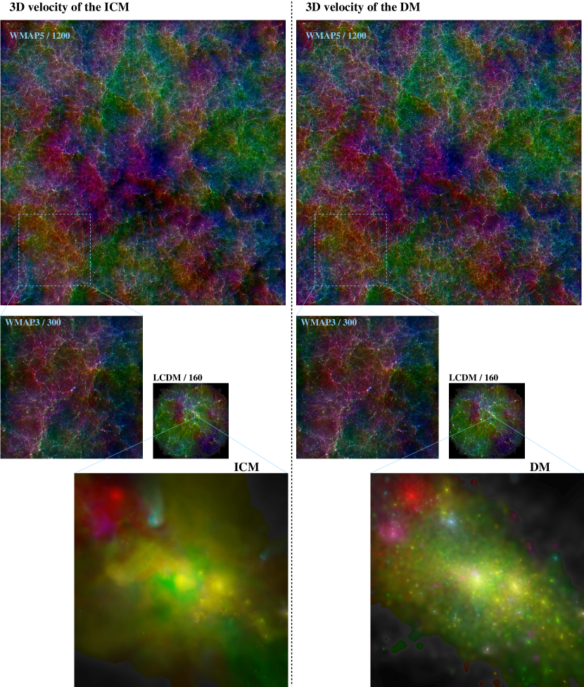
Figure 7: Visualization of velocity field the 3 different simulations using the the ray–tracing software SPLOTCH. Left side shows the ICM component, right side shows the dark matter component. The color composition reflect the three dimensional velocity field (see text for details), whereas the intensity reflects the density.

5 Relative ICM bulk motion

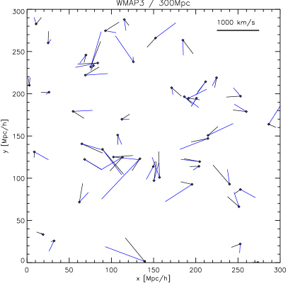
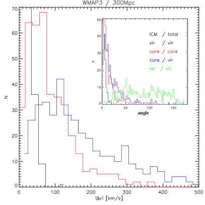
Figure 8: Shown are the different velocities of the different components within a halo. Left panel shows the velocity vectors of the ICM core compared to the mean velocity of the whole halo. Right panel shows the distribution of the angle between the velocity of the ICM component compared to the total halo measured within different regions.

While Diego et al. (2003) speculated from observation of cold fronts in galaxy clusters, that the baryonic motion (e.g. sloshing) inside of galaxy clusters could significantly affect the kSZ measurements, Nagai et al. (2003) used non radiative simulations to conclude that the effect of the ICM motions in galaxy clusters is rather mild, adding only 50-100 km/s scatter to the observed kSZ signal. Here we want to re-examine the amount of sloshing using up to date cosmological simulations which include the effect of cooling and star-formation extending previous studies by Diaferio et al. (2005) to more massive systems present in our simulations.

To give an impression of the cosmological velocity field reflected by the different components in our simulations we used the SPLOTCH package (Dolag et al., 2008), a Ray–tracing visualization tool for SPH simulations. Instead of mapping a scalar value to a color table, we mapped the three velocity components directly into the RGB colors. To obtain a logarithmic like scaling but preserve the sign of the individual velocity components we used a mapping based on the inverse of the hyperbolic sin function, e.g. $\left<r,g,b\right>\propto\mathrm{asinh}(v_{x,y,z})$. For the DM particles we calculated a smoothed density field based on all DM particles using a SPH like kernel function. The resulting Ray–tracing images, are shown in Figure 7. The left column shows the result for the ICM component, whereas the right column shows the dark matter component. Clear to see that the large scale velocity field is equally represented in the dark matter as well as ICM component, as expected. However, if one zoom into a galaxy cluster, there are striking differences in the velocity field of the two components. On one hand, within the dark matter there are more substructures (e.g. galaxies) which have individual velocities. On the other hand, and more importantly, there are quite striking, large scale velocity structures within the ICM visible, which are not reflected in the dark matter.

This is expected from the observations of ICM sloshing within the cluster potential, where velocities of up to 1000 km/s are inferred. Such velocities are quite comparable with the sloshing velocities predicted by our simulations, as will be discussed in detail in section 5.2.

5.1 Relative motions in the core

As a first step, we can divide the cluster into two parts, namely everything within the viral radius $R_{\mathrm{vir}}$ and the core (which for simplicity we define simple as the region within $0.1\times{}R_{\mathrm{vir}}$) where we will subscribe the quantities calculated within regions with vir and core respectively. For those two regions, we then can define the mass weighed mean velocity of all constituents or the mass weighed velocity of the baryonic component, which we will subscribe with total and ICM respectively. Therefore $v_{\mathrm{vir}}^{\mathrm{total}}$ correspond to the peculiar velocity of the halo, whereas $v_{\mathrm{core}}^{\mathrm{ICM}}$ correspond more to the bulk of the signal expected from measurements.

Figure 8 shows the difference of those velocities for the medium size cosmological box (WMAP3 / 300). The left panel show the position and velocity vectors for the 50 most massive clusters. Shown is the peculiar velocity (black lines) compared to the bulk of the signal expected from measurements as represented by $v_{\mathrm{core}}^{\mathrm{ICM}}$ (blue lines). Clear to see that amplitude (e.g. length of the lines, the corresponding amplitude is given in the legend in the upper right part of the plot) as well as direction are not the same and in the majority of the cases the velocity of the ICM in the center is larger than the peculiar velocity of the cluster. In some cases the direction can bee even completely opposite. The right panel shows a more quantitative result by showing the distribution of the length (main plot) as well as the angle (inlay) between the different velocities for all clusters above a mass limit of $10^{14}$ $M_{\odot}/h$. The tightest correlation (e.g. largest peak at small angles) is found when comparing $v_{\mathrm{vir}}^{\mathrm{ICM}}$ with $v_{\mathrm{vir}}^{\mathrm{total}}$ indicating that the overall mass weighted velocity of the ICM within the virial radius is typically within 50 km/s and 5 degrees of the peculiar velocity (black histogram). The difference between the motion of the total mass within the core and the ICM within the core (e.g. angle between $v_{\mathrm{core}}^{\mathrm{ICM}}$ and $v_{\mathrm{core}}^{\mathrm{total}}$) is found to be typically different by less then 100 km/s and 20 degrees (red line). The ICM velocity of the core typically is only weakly related to the peculiar velocity, typically 100 km/s but with a very pronounced tail to much larger values and the angle between $v_{\mathrm{core}}^{\mathrm{ICM}}$ and $v_{\mathrm{vir}}^{\mathrm{total}}$ encompasses typically 30 degree (blue line). The difference between the relative ICM motion inside the core and in respect to the peculiar velocity and the peculiar velocity itself is completely uncorrelated, as can be seen from the flat distribution of the angle (green line).

We conclude that overall statistically the bulk motion of the ICM (within the virial radius) is very similar than that one of the dark matter (see figure 6), however there is a significant relative motion of the ICM in respect to the dark matter in nearly every cluster, which is more pronounced within the core radius of the cluster than in the outskirts. Here we want to remind that the X-ray line emissivities are proportional to the square of the electron density and to the abundance of iron. Therefore the central part of the cluster will contribute to the bulk of the total line emission signal. On the other hand, kSZ measurements are proportional to the column density of electrons and therefore contains a significant contribution from the gas in the periphery of clusters.

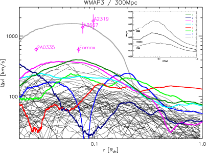
Figure 9: Radial profile (cumulative) of the velocity difference between the ICM and the dm component. Shown are every tenth profiles from all clusters above $10^{14}$ $M_{\odot}/h$ taken from the medium size cosmological box WMAP3 / 300 at $z=0$. The profiles of the 8 most massive clusters in the simulation are shown as extra, color coded lines. The data points are inferred motions of the core as imprinted in cold fronts in observed clusters. The right inlay shows the median and the 25/75 percentile when scaling the velocities of the individual clusters by the virial velocity dispersion calculated from their virial mass. For the typical mass fraction (relative to the total mass) of the different components as function of cluster centric distance see figure 12.

5.2 Radial profiles of relative motions

To quantify the effect of the ICM sloshing inside the cluster potential as expected from cosmological simulations more quantitatively, we compute the profiles of the velocity difference between the ICM and the dark matter within a given radius for all clusters more massive than $10^{14}$ $M_{\odot}/h$ from the medium size cosmological box WMAP3 / 300. The individual profiles are shown in the left panel of figure 9. Clear to see that such velocity difference at distance of the core radius is typically of order of 100 km/s with many systems reaching velocity differences of several hundreds of km/s, the most extreme ones even more than 1000 km/s. This sloshing can be compared with the velocities inferred from the observations of cold fronts in real clusters. As comparison, we over-plot the values for 4 known systems taken from Markevitch & Vikhlinin (2007) and references therein. These data points should (and actually do quite well) mark the extreme velocity differences to be expected in the simulated clusters and therefore the sloshing of the ICM in the cores of our simulated clusters is found to fairly represent the amount of sloshing found in observed systems.

The amount of sloshing is expected to be related to the depth of the potential well of the cluster and indeed, when scaling the velocity with a value of the virial velocity dispersion

$$\sigma_{v}=\sqrt{\frac{GM_{\mathrm{vir}}}{3R_{\mathrm{vir}}}}$$ (6)

expected for the different clusters according to their virial mass, the scatter in the individual profiles is strongly reduced. The inlay panel of figure 9 shows the median and the 25/75 percentile of the scaled profiles. We therefore find that the cores of the simulated galaxy clusters typically are sloshing with approximately 18% of the virial velocity dispersion, indicating that for very massive clusters this signal significantly contributes to the measurement of the peculiar velocity, typically 30% for systems with masses above $10^{15}$ $M_{\odot}/h$. This contribution drops to less than 10% for systems with masses around $10^{14}$ $M_{\odot}/h$. Therefore stacking many small systems as done in Hand et al. (2012) indeed might be a good choice to minimize the bias induced by the relative ICM motions within the clusters and groups.

Figure 10: Radial profile of kSZ for the 8 most massive halos, (x,y,z) projection each. Clear to see that the weighting by density gives very large weight to the contribution by the velocity within the core region, where the difference between the local motion of the ICM and the bulk motion of the cluster usually is largest. Color of the lines is the same as in figure 9.

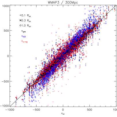
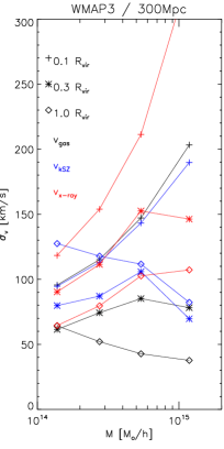
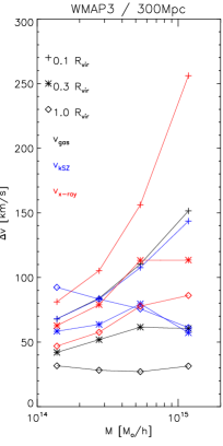
Figure 11: Difference between the peculiar velocity along the line of sight and the velocity inferred from different observables. Left panel shows a one-by-one scatter plot of all halos using the x,y and z projection of each halo. Different symbols refer to different aperture sizes (crosses = core, stars = $0.3\times{}R_{\mathrm{vir}}$, diamonds are within $R_{\mathrm{vir}}$). Different colors refer to X-ray (red), kSZ including X-ray temperature bias (blue) and ideal kSZ measurements (black). The middle panel shows the bias in form of the RMS of the velocity difference as function of the mass of the cluster and the right panel shows the bias in form of the velocity difference.

6 Impact on observations

It is outside the scope of this paper to include realistic observational effects through mimicking instruments or background. However, in this section we want to evaluate the principal limits up to which accuracy we can infer the peculiar velocity of clusters from observables, given the complex thermal and dynamical structure within galaxy clusters. We also want to evaluate this in the light of different observables, which intrinsically weight the radially varying signal differently. Especially we want to investigate the influence of the radial dependent relative motion of the ICM in respect to the dark mater halo when measuring the ICM motion via kSZ effect or by measuring the shift of the iron line with detailed X-ray spectroscopy.

6.1 Spacial distribution of the observable signal

To give an impression of the actual spacial distribution of the signal we discuss the appearance of the different observables in the Appendix B1, where Figure 18 a visualize the maps of different observable. To show, how far out from the cluster center the the internal motions affect the kinematic signal, Figure 10 shows the radially averaged, cumulative profile of the kinetic SZ effect. The different colors are the 8 different clusters, whereas the 3 different lines for each cluster are for three different projection directions of these four clusters. Clear to see that the internal motions are significantly influencing the kinematic signal up to a radius of between 0.3 and 0.5 times $R_{\mathrm{vir}}$.

6.2 The observed bulk velocity

To infer the mean bulk motion of the ICM from the kinetic SZ signal, one has to assume, that the observed kinetic SZ signal, integrated over a certain aperture $A$

$$\left<w\right>_{A}=\int_{A}\frac{\sigma_{t}}{c}\int n_{e}v_{r}\mathrm{d}l\approx\int_{A}\frac{\sigma_{t}\left<v_{r}\right>}{c}\int n_{e}\mathrm{d}l$$ (7)

can be interpreted as the the signal of the mean (radial) velocity $\left<v_{r}\right>$ if the ICM, weighted with the mean surface mass density. The later can be obtained from the integrated thermal SZ signal within the same aperture

$$\left<y\right>_{A}=\int_{A}\frac{k\sigma_{T}}{m_{e}c^{2}}\int n_{e}T\mathrm{d}l\approx\int_{A}\frac{k\sigma_{T}\left<T\right>}{m_{e}c^{2}}\int n_{e}\mathrm{d}l$$ (8)

with the Boltzmann constant $k$, the Thomson cross-section $\sigma_{T}$, the speed of light $c$, the mass of the electron $m_{e}$ and the temperature and density of the ICM $T$ and $n_{e}$. Assuming that one can infer $\left<T\right>$ from X-ray observations, one can combine these two measurements to obtain the mean velocity $\left<v_{r}\right>$ within the aperture $A$.

The aperture $A$ here can either be the beam in case the cluster could be resolved by the observations or the area of the cluster itself in case it is not resolved. In general, this means that the observed velocity $\left<v_{r}\right>$ within the aperture $A$ therefore differ from the mean, mass weighted velocity by the difference between the mass weighted temperature (from $\left<y\right>_{A}$) and the temperature inferred from X-ray observations. For a more detailed discussion see Diaferio et al. (2005). The relation of these two temperatures is not trivial, as the X-ray temperature is weighted by the emission measure and comes from a fit of an emission spectra usually assuming a single temperature. For the complex temperature structure of galaxy clusters this can induce a significant bias (see Mathiesen & Evrard, 2001; Mazzotta et al., 2004; Vikhlinin, 2006) This bias has to be either corrected using simulations, or can be minimized by using spacial resolved X-ray temperature maps (which still leaves the multi temperature structure along the line of sight) but allows to re-construct the 3D temperature profile using iterative reconstruction methods (see Ameglio et al., 2007, and references therein)

Alternatively one can also use multi-temperature model (see Kaastra et al., 2004; Biffi et al., 2012) to obtain the temperature distribution of the ICM. For our purpose, we will investigate two extreme cases. In the most optimistic case, we assume that this bias can be eliminated completely and we take the mass weighted mean velocity along the line of sight (labeled as ICM in figure 11) within the aperture $A$. In the most pessimistic case, we include the temperature bias as inferred from the simulation (labeled as kSZ in figure 11).

In case the mean ICM velocity is inferred from X-ray spectroscopic measurements (labeled as X-ray in figure 11), the observed velocity correspond to the mean, emission weighted ICM velocity, which due to the steep radial emission profile is biased towards the mean velocity within the cluster core.

As the SZ measurements are not dependence on the distance, we use the extend of the simulation (e.g. 300 Mpc/h) along the line of sight when measuring quantities within the aperture $A$. As the X-ray signal is redshift and distance dependent, we use only the local signal of the cluster when calculating the temperature bias and the emission weighted mean velocity within the same aperture $A$. We restrict ourselves to explore 3 different apertures, namely the core (corresponding to $0.1\times{}R_{vir}$), a region spanning $0.3\times{}R_{vir}$ and the region encompassing the virial radius.

In the left panel of figure 11 we show a point by point comparison of the difference of the observed velocity along the line of sight and the peculiar velocity along the line of sight for all 9 combinations of measurements and apertures. The middle panel of figure 11 shows the root mean square (RMS) scatter between the different observed velocities and the peculiar velocity of the cluster and the right panel shows the mean between the different observed velocities and the peculiar velocity. Clear to see that the X-ray based methods have larger scatter, as they emphasize the relative motions of the ICM within the cores. Here it is also clearly visible, that going to larger masses increases the difference, because more massive systems show stronger sloshing motions as shown earlier. This effect dominates all measurements which depend on small, central apertures. However, larger apertures show an opposite effect when going to larger clusters. This is because within a more massive clusters, the larger volume probed along the line of sight overcomes the increased bias within the central region.

We also note that the knowledge of the true temperature of the system is quite important. Any bias in the measured temperature leads to a bias in the inferred kSZ signal, as can be clearly be seen for the blue points in the left panel of figure 11, where we assumed the typical temperature bias as inferred from simulations. Note also that especially in the systems with the largest velocity, the distribution of the individual points clearly shows deviations from a linear relation which indicates that in these cases calibrating a simple bias is not enough to recover the real signal.

6.3 Stars as proxies for the bulk motions of clusters

Finally we investigate alternatively to use the collissionless components of the baryonic content of clusters as probe of the peculiar motion of the system. To do so, we are using the highest resolutions simulation in our set. This allows us to study in detail the stellar component of the simulations. Thereby, the larger, underlying resolution of this simulation allows us – after subtracting all member galaxies – to use the velocity distribution of the remaining stars to characterize two, dynamically well-distinct stellar components within the simulated galaxy clusters. These differences in the dynamics is then used to apply an unbinding procedure similar than applied when identifying the member galaxies and lead to a spatial separation of the two components into stars belonging to the central galaxy and stars belonging to the diffuse stellar component (see Dolag et al., 2010, for details). This then can be used to investigate if, and in case which, stellar component might be the best proxy to measure the real peculiar motion of the cluster.

Although in this simulation, the most massive galaxy cluster is resolved with nearly one million particles, we will present the results when averaging over the 24 most massive clusters within the LCDM / 160 simulation, as the radial profiles obtained from from individual clusters turn out to be still too noisy. The different stellar components have different radial distributions and reflect different amount of the baryonic component of galaxy clusters. Figure 12 shows the relative mass fraction of the different components as function of radius. In the very center part, the stars from the central galaxy (cD) are dominating, outside of that region the dark matter (DM) is dominating by far. The ICM does not play an important role within the core and has a roughly constant fraction outside of it. In the very outer part, the total mass associated to the satellite galaxies (SUB) dominates, whereas the contribution of the stellar mass of the sub-structures (GAL) as well as the diffuse stellar component (ICL) fall radially faster of than the dark matter.

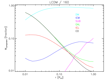
Figure 12: Mass fraction of the different components of the clusters. Shown is the average over the 24 most massive clusters in the high resolution, LCDM / 160 simulation. Here SUB devotes all material within identified sub structures (excluding the main halo which also includes cD and ICL). GAL devotes all stellar components of sub structures (but including the cD).

Finally, figure 13 shows how these different components trace the underlying peculiar motion of the cluster as a whole. We again show the result averaged over the 24 most massive clusters from the LCDM / 160 simulation, where we normalized the velocity differences of the individual clusters by their virial velocity dispersion obtained from equation (6) before averaging, in the same spirit than done in the right panel of figure 9. In the central region, the relative motion of the dark matter component is slightly less than that one of the ICM component (around 25% and 30% of the virial velocity dispersion, respectively) but rapidly approaches the peculiar velocity of the halo with only a very small remaining bias at large distances, originating from the small, mass weighed contribution of the baryonic component. The best tracer of the peculiar motion of the cluster close to the center seems to be the stellar component of the central galaxy, which shows the smallest relative velocity (ca. 20% of the virial velocity dispersion). As already noted earlier, the mean velocity of the galaxies is a quite bad tracer of the peculiar motion of the cluster, especially when going to the outer parts where more and more galaxies are contributing and the weight of the central galaxy decreases. There the relative motion reaches up to 35% of the virial velocity dispersion. The diffuse stellar component performs here much better (having only a relative motion of roughly 20% of the virial velocity dispersion). This is still significantly larger that the residual motions of the ICM at this large distances and it remains to be investigated if that remaining signal is dominated from the outer parts of the otherwise separately identified galaxies, which then might be associated to the diffuse component or if the velocity difference is driven by remaining streams of already destroyed galaxies. It has also to be stressed that the dispersion among the 24 individual is quite substantial, as can be seen from the exemplary error bars displayed at small and large radii. Here we conclude that although having a large offset, the stellar component of the central galaxy would give relatively the best proxy of the overall peculiar velocity of the cluster at small, cluster centric distances, whereas at large distance the ICM measured by the kinetic SZ effect will be still the best indicator.

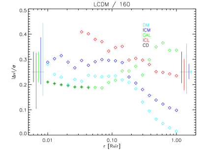
Figure 13: Profiles (cumulative) of the relative motion of different components with respect to the underlying peculiar motion of the cluster. Shown is the again average over the 24 most massive clusters in the LCDM / 160 simulation. Components are the same than in figure 12. The error bars left and right to the curves show the 25/75 percentiles typical at small (left) and large (right) radii.

7 Application to pairwise velocity measures

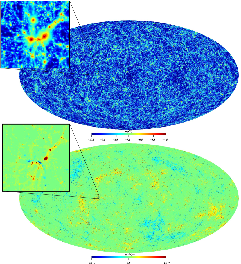
Figure 14: Full sky projections of thermal (upper panel) and kinetic (lower panel) signal taken exemplary from the last shell (e.g. $z=0.14-0.16$) integrated through the WMAP5/1200 simulation. The inlays show a zoom onto one of the prominent structures within that shell. Clear to see the large scale peculiar velocity patterns reflected in the kinetic signal, which inside the structures get perturbed by the local motions within the super cluster structure as well s internal motions within some of the clusters.

To verify the findings presented in (Hand et al., 2012) we where using SMAC (Dolag et al., 2005) to produced full sky maps from the simulations. Here we stack the simulation of the local universe (LCDM/160) into the large, cosmological box (WMAP5/1200). We constructed the full sky maps stacking consecutive shells through the cosmological boxes taken at the evolution time corresponding to the distance. Without replicating the box we thereby reached a maximum distance of $z=0.16$. The according maps for the thermal and kinetic SZ effect are displayed in figure 14, which shows exemplary the last shell taken from the WMAP5/1200 simulations. The maps are based on a HEALPIx representation of the full sky (Górski et al., 1998) using a resolution of $n_{\mathrm{side}}=2048$ which leads to a pixel size roughly corresponding to the binning radius of the maps of the individual groups and clusters used in Hand et al. (2012).

We then identified all galaxies (e.g. sub-halos) in the simulations. Applying a cut in the maximum circular velocity ($v_{\mathrm{max}}$) we selected the most massive galaxies, which represent the center of groups and clusters. Analog to Hand et al. (2012), from the three dimensional position of these galaxies, $\mn@boldsymbol{r}_{i}$ we define the pairwise signal as

$$p_{\mathrm{kSZ}}(r)=-\frac{\sum_{i<j}(T_{i}-T_{j})c_{ij}}{\sum_{i<j}c_{ij}^{2}}$$ (9)

whereas $T_{i}$ and $T_{j}$ are the pixel values of the full sky map towards the position of galaxies $i$ and $j$, respectively, and $c_{ij}$ is constructed from the three dimensional positions $\mn@boldsymbol{r}_{i}$ and $\mn@boldsymbol{r}_{j}$ according to

$$c_{ij}=\mn@boldsymbol{r}_{ij}\dot{\frac{\mn@boldsymbol{r}_{i}+\mn@boldsymbol{r}_{j}}{2}}.$$ (10)

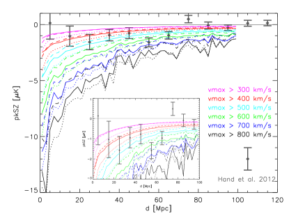
Figure 15: Pairwise signal for different cuts in maximum circular velocity (e.g. Mass) of galaxies from the simulations using the kinetic SZ map directly produced from the hydrodynamical simulations (solid lines) compared with the observational data points taken from Hand et al. (2012). The dotted lines shows the estimated signal when using the combination of thermal SZ, temperature and bulk velocity of the halo. The dashed line shows the same but calibrates the optical depth to match the signal when using all halos. The inlay shows a zoom into the range where the observational signal is detected.

Figure 15 shows the result from this procedure compared to the observational data points. When restricting to more massive systems, the signal is, as expected, much stronger and extend to much larger distances. However, the results obtained from the hydrodynamical simulations are in good agreement with the signal seen in the observations. The Luminosity cut applied to the observations should correspond to a limiting halo mass in the sample of $M_{200c}\approx 4.1\times 10^{13}M_{\odot}$ (Hand et al., 2012), which corresponds roughly to a maximum, circular velocity of the simulated halos of $\approx 500\mathrm{km/s}$. Note that the theoretical curves are based on the real, three dimensional position of the clusters/groups and the calculation does not include observational effects like the contribution of the peculiar velocity of the individual clusters/group to their distance estimate or the averaging of the signal at small scales due to the beam. Especially at the smallest bins it can be expected that this would lead to a change of the signal.

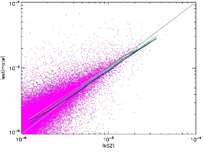
Figure 16: Pixel by pixel comparison of the kinetic SZ signal obtained directly from the hydrodynamical simulation with the estimated signal based on the bulk velocity of the halo. Shown is the signal of all halos selected wit a circular velocity larger than $300\mathrm{km/s}$. Additional, the mean is shown for selecting different halos based on their circular velocity as done is figure 15.

We also produced a mass weighed temperature map which then can be used when combining equation (5) and (6) to get an estimated kinetic SZ signal base on the halo bulk velocity and the thermal SZ signal

$$\left<w\right>_{A}=v_{\mathrm{halo}}\frac{\left<y\right>_{A}}{\left<T\right>_{A}}\frac{m_{e}c}{k}.$$ (11)

The resulting signal from this estimation can be compared pixel by pixel to the kinetic SZ signal which was obtained directly from the hydrodynamical simulation. The result of that comparison for all halos is shown in figure 16. Clear to see that there is not only a large scatter but also systematic trend which is related by approximating the optical depth through the mean temperature and the mean thermal SZ measured in each pixel. The expected pairwise signal from this approximation is shown as dotted line in figure 15. The bias induced by approximating the optical depth of the individual systems by combining their thermal SZ signal with the mean temperature of these systems can in principal be calibrated based on the hydrodynamical simulations itself. We find that a reduction of 30% of the estimated optical depth leads to a very good agreement between the true and the estimated signal, especially when looking at the signal obtained when including all halos, as can be seen by the dashed lines in figure 15, which falls basically on top of the signal obtained from the real kinetic SZ signal extracted from the maps. However, when going to more massive systems it can be seen that the true kinetic SZ signal is significantly larger than the one estimated from the bulk velocity of the halo, again indicating that in massive systems internal motions of the ICM in respect to the bulk motion of the halo itself are contributing significantly to the expected kinetic SZ signal.

8 Conclusions

We used a large set of cosmological, hydrodynamical simulations, which cover very large cosmological volume, hosting a large number of rich clusters of galaxies, as well as moderate volumes where the internal structures of individual galaxy clusters can be resolved with very high resolution to investigate, how the presence of baryons and their associated physical processes like cooling and star-formation are affecting the systematic difference between mass averaged velocities of dark matter and the ICM inside a cluster and how that is reflected in observables like the kinematic SZ effect.

Our main findings are:

• The peculiar velocity of galaxy clusters are, as expected, independent of mass and redshift following a Maxwell distribution. However, being able to probe very large cosmological volumes, we could demonstrate that the characteristic velocity of this distribution is not a fixed value but depends on the local, large scale over-density within a sphere of 20 Mpc ($\delta_{20\mathrm{Mpc}}$) as

  $$\sigma_{v}\;[\mathrm{km}/\mathrm{s}]\;=185\times\mathrm{exp}\left(\delta_{20\mathrm{Mpc}}/10\right)$$ (12)

  and thereby typical peculiar velocities (which are $\approx$ 410 km/s for the most recent cosmological parameters) increase by a factor of 2 within super cluster regions.

• Also in merging systems the relative velocity of the clusters is strongly increase and typically exceeds values of 1000 km/s in the moment when the virial sizes of the two systems touch. It has to be also noted that even in the larges box of or simulation campaign (WMAP5 / 1200) all cluster pairs with distances less than three times their virial size are approaching each other.

• Relative ICM motions in the center of galaxy clusters can in some cases exceed the peculiar motion of the cluster as a whole. We find relative motions (so called sloshing) of the ICM up to 1000 km/s, in good agreement with observations. This sloshing motions are scaling with the virial velocity dispersion of the clusters and typically 25% of the clusters show sloshing motions of 20% of the virial velocity dispersion within their core which decrease to 9% averaged over the virial region. The relative motions of the core compared to the peculiar velocity thereby are completely uncorrelated.

• When measuring the peculiar motion of the galaxy cluster by combining the kinematic and thermal SZ measurement, the additional bias between the mass weighted temperature (entering the thermal SZ signal) and the temperature inferred from X-ray observations (which is in addition needed) further increases the scatter between the inferred velocity and the true, peculiar velocity. The combination of the dependence of the relative motions of the ICM with cluster mass and the dependence of the observed signal with the size of the observational aperture leads to a mass dependence of this scatter. Whereas for less massive clusters (e.g. $10^{14}M_{\odot}/h$), the induced scatter is of order 60-90 km/s dependent on the aperture and the size of the temperature bias, for very massive systems (e.g. $10^{14}M_{\odot}/h$), the scatter is between 50 km/s and 200 km/s, depending mainly on the size of the aperture. In case the signal is inferred from X-ray data only (e.g. using high resolution microcaloimeters), the scatter for small apertures is even significantly larger.

• When looking at the stellar components of the cluster it is important to note that the mean velocity of the galaxy population even when averaging within the virial region is a very bad indicator of the peculiar velocity of the system. Interestingly, although obtained only from the central part of the cluster, the stellar component of the central galaxy gives a much better indicator of the peculiar motion of the cluster, however the relative difference in that case is still a factor of two worse than the mean velocity obtained from the ICM within the virial region.

• The pairwise velocity signal as measured in Hand et al. (2012) is in qualitative agreement with the expectations from hydrodynamical simulations, although it strongly depends on the mass cut applied to the selected clusters/groups. There is a significant (30%) bias introduced by the estimation of the optical depth based on temperature and thermal SZ signal. Additional, when restricting to massive system to increase the signal, internal velocities of the ICM are giving a significant extra contribution to the observed kinetic SZ effect.

Given the improved sensitivity of current instruments it might be expected that the kinetic SZ signal in massive clusters will be detected soon. However, it has to be kept in mind that, as we clearly demonstrated, the internal motions of the ICM within the central part in respect to the galaxy cluster as whole is more pronounced in massive systems, where such internal motions by far exceed the expected bulk motion, which leads to an unavoidable systematical error in the inferred peculiar velocities of the halos which is connected to the relative motion between the dark matter and the ICM. This will dominate the signal unless one integrates over relatively large area. However, when integrating over larger area, understanding and correcting for the the bias between mass weighted and measured (via X-ray) temperature gets more crucial, as one averages over a larger range in temperature structures within the ICM. Measurements of the ICM velocity using X-ray spectra will be even more affected, as they give additional weight to the central regions. Therefore we conclude that measuring the velocity of the ICM in the central regions of galaxy clusters will give very interesting insights into the dynamics of galaxy clusters, however one has to be carefully when associating the peculiar velocity of galaxy clusters with such measurements.

Appendix A Peculiar velocity of halos in DM and csf simulations

The distribution of the overall peculiar motions of galaxy clusters reflect the large scale velocity field, which still probes the linear regime of structure formation. Therefore we do not expect the presence of baryonic components and their associated physical processes (like cooling, star-formation and stellar feedback) to influence the overall peculiar velocities of galaxy clusters. This is also demonstrated in figure 17, which shows (as in the left panel of figure 2) the distribution of cluster peculiar velocities for different cut in cluster mass from the large cosmological box WMAP5 / 1200, comparing the simulation including cooling and star-formation (solid line) with the dark matter only simulation of he same cosmological box (dashed lines).

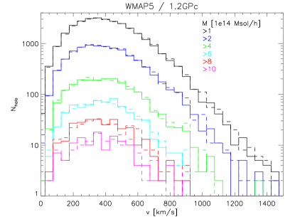
Figure 17: Histogram of the peculiar motion of galaxy clusters from the large cosmological box WMAP5 / 1200 Comparing DM and csf simulation. Shown are the histograms for clusters above $10^{14}$, $2\times 10^{14}$, $4\times 10^{14}$, $6\times 10^{14}$, $8\times 10^{14}$ and $10^{15}$ $M_{\odot}/h$.

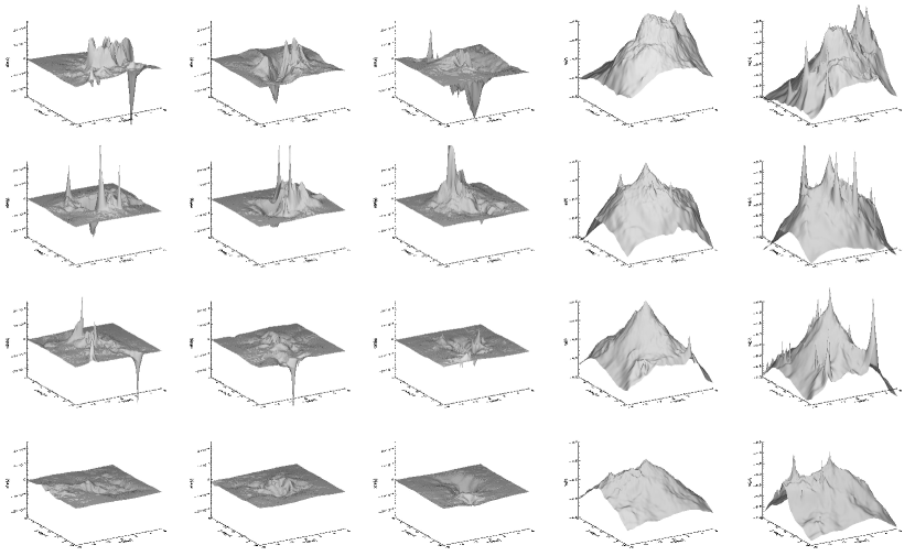
Figure 18: Visualization of the kSZ, tSZ and X-ray SB for the 4 most massive clusters within the medium size cosmological box WMAP3 / 300 (4 rows). From left to right are the 3 different spacial projection directions (x,y,z) of the kSZ (shown is asinh(w)), the tSZ (x projection, shown is log10(y)) and the X-ray surface brightness (x projection, shown is log10(SB)). Displayed is a 1.5x1.5 Mpc region centered on the clusters.

Appendix B Spacial distribution of the observable signal

To give an impression of the actual spacial distribution of the signal we show in Figure 18 a visualize the maps of different observable, where the height in the 3D plot correspond to the strength of the signal. The region shown is a 1.5Mpc times 1.5Mpc region centered on the individual clusters. Shown is the kinetic (first three rows) and thermal SZ effect (4th row) as well as the X-ray surface brightness of the four most massive clusters from the medium size cosmological box WMAP3 / 300. The internal motions of the different parts of the clusters can be clearly seen in the different minima’s and maxima’s of the maps. Very sharp and isolated features are representing sub structures, which still have a baryon content left which is not yet stripped by the cluster atmosphere. In line with previous findings, only a very small number of the hundreds of resolved substructures within the cluster have still some residual gas (see also Dolag et al., 2009) which thereby contributes to the overall kSZ signal of the ICM. Due to the significant internal bulk motions within the ICM also large scale features can be clearly seen. Within the thermal SZ signal, the substructures with still host noticeable amount of gas do not stick out so much compared to the ICM, demonstrating that the strong signals in the kinetic effect are dominated by the large, relative motion and are not due to a larger comtonization parameter of the gas within such substructures. As most of the large scale structures within the cluster are approximately in pressure equilibrium, the thermal SZ effect shows in comparison a much more regular structure. Also clear to see that the X-ray signal, due to its density square dependence falls off much more rapidly than the thermal SZ signal.

References

- Ameglio et al. (2007) Ameglio S., Borgani S., Pierpaoli E., Dolag K., 2007, MNRAS, 382, 397
- Ascasibar & Markevitch (2006) Ascasibar Y., Markevitch M., 2006, ApJ, 650, 102
- Bahcall et al. (1994) Bahcall N. A., Gramann M., Cen R., 1994, ApJ, 436, 23
- Biffi et al. (2012) Biffi V., Dolag K., Böhringer H., Lemson G., 2012, MNRAS, 420, 3545
- Bryan & Norman (1998) Bryan G. L., Norman M. L., 1998, ApJ, 495, 80
- Bulbul et al. (2012) Bulbul G. E., Smith R. K., Foster A., Cottam J., Loewenstein M., Mushotzky R., Shafer R., 2012, ApJ, 747, 32
- Churazov et al. (2001) Churazov E., Brüggen M., Kaiser C. R., Böhringer H., Forman W., 2001, ApJ, 554, 261
- Churazov et al. (2012) Churazov E., Vikhlinin A., Zhuravleva I., Schekochihin A., Parrish I., Sunyaev R., Forman W., Böhringer H., Randall S., 2012, MNRAS, 421, 1123
- De Boni et al. (2011) De Boni C., Dolag K., Ettori S., Moscardini L., Pettorino V., Baccigalupi C., 2011, MNRAS, 415, 2758
- De Boni et al. (2012) De Boni C., Ettori S., Dolag K., Moscardini L., 2012, ArXiv e-prints
- Diaferio et al. (2005) Diaferio A., Borgani S., Moscardini L., Murante G., Dolag K., Springel V., Tormen G., Tornatore L., Tozzi P., 2005, MNRAS, 356, 1477
- Diaferio et al. (2000) Diaferio A., Sunyaev R. A., Nusser A., 2000, ApJ, 533, L71
- Diego et al. (2003) Diego J. M., Mazzotta P., Silk J., 2003, ApJ, 597, L1
- Dolag et al. (2009) Dolag K., Borgani S., Murante G., Springel V., 2009, MNRAS, 399, 497
- Dolag et al. (2005) Dolag K., Hansen F. K., Roncarelli M., Moscardini L., 2005, MNRAS, 363, 29
- Dolag et al. (2010) Dolag K., Murante G., Borgani S., 2010, MNRAS, 405, 1544
- Dolag et al. (2008) Dolag K., Reinecke M., Gheller C., Imboden S., 2008, NJoP, submitted
- Dolag et al. (2005) Dolag K., Vazza F., Brunetti G., Tormen G., 2005, MNRAS, 364, 753
- Fedeli et al. (2012) Fedeli C., Dolag K., Moscardini L., 2012, MNRAS, 419, 1588
- Frenk et al. (1999) Frenk C. S., White S. D. M., Bode P., Bond J. R., Bryan G. L., Cen R., Couchman H. M. P., Evrard A. E., Gnedin N., Jenkins A., Khokhlov A. M., Klypin A., 1999, ApJ, 525, 554
- Górski et al. (1998) Górski K. M., Hivon E., Wandelt B. D., 1998, ‘Analysis Issues for Large CMB Data Sets’, 1998, eds A. J. Banday,R. K. Sheth and L. Da Costa, ESO, Printpartners Ipskamp, NL, pp.37-42 (astro-ph/9812350); Healpix HOMEPAGE: http://www.eso.org/science/healpix/
- Grossi et al. (2009) Grossi M., Verde L., Carbone C., Dolag K., Branchini E., Iannuzzi F., Matarrese S., Moscardini L., 2009, MNRAS, 398, 321
- Haardt & Madau (1996) Haardt F., Madau P., 1996, ApJ, 461, 20
- Hand et al. (2012) Hand N., Addison G. E., Aubourg E., Battaglia N., Battistelli E. S., Bizyaev D., Bond J. R., Brewington H., Brinkmann J., Brown B. R., Das S., Dawson K. S., Devlin M. J., Dunkley J., Dunner R. e. a., 2012, Physical Review Letters, 109, 041101
- Hoffman & Ribak (1991) Hoffman Y., Ribak E., 1991, ApJ, 380, L5
- Iapichino & Niemeyer (2008) Iapichino L., Niemeyer J. C., 2008, MNRAS, 388, 1089
- Inogamov & Sunyaev (2003) Inogamov N. A., Sunyaev R. A., 2003, Astronomy Letters, 29, 791
- Kaastra et al. (2004) Kaastra J. S., Tamura T., Peterson J. R., Bleeker J. A. M., Ferrigno C., Kahn S. M., Paerels F. B. S., Piffaretti R., Branduardi-Raymont G., Böhringer H., 2004, A&A, 413, 415
- Keisler & Schmidt (2012) Keisler R., Schmidt F., 2012, ArXiv e-prints
- Kolatt et al. (1996) Kolatt T., Dekel A., Ganon G., Willick J. A., 1996, ApJ, 458, 419
- Komatsu et al. (2009) Komatsu E., Dunkley J., Nolta M. R., Bennett C. L., Gold B., Hinshaw G., Jarosik N., Larson D., Limon M., Page L., Spergel D. N., Halpern M., Hill R. S., Kogut A., Meyer S. S., Tucker G. S., Weiland J. L., Wollack E., Wright E. L., 2009, ApJS, 180, 330
- Markevitch et al. (2004) Markevitch M., Gonzalez A. H., Clowe D., Vikhlinin A., Forman W., Jones C., Murray S., Tucker W., 2004, ApJ, 606, 819
- Markevitch & Vikhlinin (2007) Markevitch M., Vikhlinin A., 2007, Phys. Rep., 443, 1
- Mathiesen & Evrard (2001) Mathiesen B. F., Evrard A. E., 2001, ApJ, 546, 100
- Mathis et al. (2002) Mathis H., Lemson G., Springel V., Kauffmann G., White S. D. M., Eldar A., Dekel A., 2002, MNRAS, 333, 739
- Mazzotta et al. (2004) Mazzotta P., Rasia E., Moscardini L., Tormen G., 2004, MNRAS, 354, 10
- Nagai et al. (2003) Nagai D., Kravtsov A. V., Kosowsky A., 2003, ApJ, 587, 524
- Paul et al. (2011) Paul S., Iapichino L., Miniati F., Bagchi J., Mannheim K., 2011, ApJ, 726, 17
- Planck Collaboration (2012) Planck Collaboration 2012, ArXiv e-prints
- Rasia et al. (2004) Rasia E., Tormen G., Moscardini L., 2004, MNRAS, 351, 237
- Reid et al. (2010) Reid B. A., Verde L., Dolag K., Matarrese S., Moscardini L., 2010, JCAP, 7, 13
- Roediger et al. (2011) Roediger E., Brüggen M., Simionescu A., Böhringer H., Churazov E., Forman W. R., 2011, MNRAS, 413, 2057
- Roncarelli et al. (2010) Roncarelli M., Moscardini L., Branchini E., Dolag K., Grossi M., Iannuzzi F., Matarrese S., 2010, MNRAS, 402, 923
- Salpeter (1955) Salpeter E. E., 1955, ApJ, 121, 161
- Sanders et al. (2011) Sanders J. S., Fabian A. C., Smith R. K., 2011, MNRAS, 410, 1797
- Schuecker et al. (2004) Schuecker P., Finoguenov A., Miniati F., Böhringer H., Briel U. G., 2004, A&A, 426, 387
- Simionescu et al. (2012) Simionescu A., Werner N., Urban O., Allen S. W., Fabian A. C., Sanders J. S., Mantz A., Nulsen P. E. J., Takei Y., 2012, ArXiv e-prints
- Spergel et al. (2007) Spergel D. N., Bean R., Doré O., Nolta M. R., Bennett C. L., Dunkley J., Hinshaw G., Jarosik N., Komatsu E., Page L., Peiris H. V., Verde L., Co-Authors ., 2007, ApJS, 170, 377
- Springel (2005) Springel V., 2005, MNRAS, 364, 1105
- Springel & Hernquist (2002) Springel V., Hernquist L., 2002, MNRAS, 333, 649
- Springel & Hernquist (2003) Springel V., Hernquist L., 2003, MNRAS, 339, 289
- Springel et al. (2001) Springel V., White S. D. M., Tormen G., Kauffmann G., 2001, MNRAS, 328, 726
- Springel et al. (2001) Springel V., Yoshida N., White S. D. M., 2001, New Astronomy, 6, 79
- Sunyaev et al. (2003) Sunyaev R. A., Norman M. L., Bryan G. L., 2003, Astronomy Letters, 29, 783
- Sunyaev & Zeldovich (1980) Sunyaev R. A., Zeldovich I. B., 1980, MNRAS, 190, 413
- Tornatore et al. (2007) Tornatore L., Borgani S., Dolag K., Matteucci F., 2007, MNRAS, 382, 1050
- Tornatore et al. (2004) Tornatore L., Borgani S., Matteucci F., Recchi S., Tozzi P., 2004, MNRAS, 349, L19
- Vazza et al. (2011) Vazza F., Brunetti G., Gheller C., Brunino R., Brüggen M., 2011, A&A, 529, A17+
- Vazza et al. (2009) Vazza F., Brunetti G., Kritsuk A., Wagner R., Gheller C., Norman M., 2009, A&A, 504, 33
- Vazza et al. (2006) Vazza F., Tormen G., Cassano R., Brunetti G., Dolag K., 2006, MNRAS, 369, L14
- Vikhlinin (2006) Vikhlinin A., 2006, ApJ, 640, 710
- Zitrin et al. (2012) Zitrin A., Bartelmann M., Umetsu K., Oguri M., Broadhurst T., 2012, ArXiv e-prints
- ZuHone et al. (2010) ZuHone J. A., Markevitch M., Johnson R. E., 2010, ApJ, 717, 908