The intergalactic Newtonian gravitational field and the shell theorem

The release of the 2MASS Redshift Survey (2MRS), with it’s 44599 galaxies allows the deduction of the galaxy’s masses in nearly complete sample. A cubic box with side of 37 Mpc containing 2429 galaxies is extracted and the Newtonian gravitational field is evaluated both at the center of the box as well in 101 x 101 x 101 grid points of the box. The obtained results are then discussed at the light of the shell theorem which states that at the internal of a sphere the gravitational field is zero.
keywords
methods: statistical; cosmology: observations; (cosmology): large-scale structure of the Universe

1 Introduction

The determination of the gravitational field in cosmology oscillates between the Newton law and various type of modifications to this law. The reference formula is the Newtonian force

$$F=-G\frac{mM}{r^{2}}\quad,$$ (1)

where $G$ is the gravitational constant, $M$ the first mass, $m$ the second mass and $r$ the distance between the two masses. The enormous progresses in the observations of the spatial distribution of galaxies point toward a cellular structure, i.e. the galaxies are situated on the surfaces of bubbles, rather than to be aggregated in a random structures, see Coil (2012). In the limiting case in which all the galaxies were situated on the surfaces of spheres the gravitational forces should be zero due to the shell theorem or nearly zero due to the fact that the galaxies are distributed in a discrete way rather than in a continuous way. This paper describes in Section 2 two astronomical catalogs which allow to calibrate the size of the cosmic voids. Section 3 is devoted to the study of the photometric properties of of a nearly spherical distribution of galaxies and to a careful analysis of completeness connected with the selected astronomical catalog. Section 4 contains the evaluation of the Newtonian gravitational field in a box of 37 $Mpc$ in which the boundary conditions are properly evaluated. Section 5 reports a comparison between three ideal structures and a real void as extracted from a slices oriented catalog.

2 Observations

This section processes the Sloan Digital Sky Survey Data Release 7 (SDSS DR7), see Abazajian et al. (2009), and the 2MASS Redshift Survey (2MRS), see Huchra et al. (2012).

2.1 Observed statistics of the voids

The distribution of the effective radius between the galaxies of SDSS DR7 has been reported in Pan et al. (2011). This catalog contains 1054 voids and Table 1 reports their basic statistical parameters.

Table 1: The statistical parameters of the effective radius in SDSS DR7.

$$\begin{array}[]{lc}\hline\cr\hline\cr\vskip 3.0pt plus 1.0pt minus 1.0pt\cr parameter&value\\ \vskip 3.0pt plus 1.0pt minus 1.0pt\cr mean&18.23h^{-1}~{}Mpc\\ \vskip 3.0pt plus 1.0pt minus 1.0pt\cr variance&23.32h^{-2}~{}Mpc^{2}\\ \vskip 3.0pt plus 1.0pt minus 1.0pt\cr standard~{}deviation&4.82h^{-1}~{}Mpc\\ \vskip 3.0pt plus 1.0pt minus 1.0pt\cr kurtosis&0.038\\ \vskip 3.0pt plus 1.0pt minus 1.0pt\cr skewness&0.51\\ \vskip 3.0pt plus 1.0pt minus 1.0pt\cr maximum~{}value&34.12h^{-1}~{}Mpc\\ \vskip 3.0pt plus 1.0pt minus 1.0pt\cr minimum~{}value&9.9h^{-1}~{}Mpc\\ \vskip 3.0pt plus 1.0pt minus 1.0pt\cr\hline\cr\hline\cr\end{array}$$

2.2 The 2MASS

The 2MASS is a catalog of galaxies which has instruments in the near-infrared J, H and K-bands (1-2.2 $\mu$ m) and therefore detects the galaxies in the so called “Zone of Avoidance,” see Jarrett (2004); Crook et al. (2007). At the moment of writing the 2MRS consists of 44599 galaxies with redshift in the interval $0\leq z\leq 0.09$, see Huchra et al. (2012). The catalog contains the galactic latitude, the galactic longitude and the expansion velocity; from these three parameters is possible to deduce the Cartesian coordinates, $X,Y$ and $Z$ expressed in $Mpc$. Figure 1 reports a cut of a given thickness of 2MRS where $\Delta$ express the thickness of the cut and $N_{G}$ the number of selected galaxies.

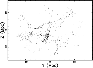
Figure 1: Cut of the 3D spatial distribution of 2MRS in the $X=0$ plane when $\Delta=$ 10 Mpc, the squared box has a side of 148 $Mpc$ and $N_{G}$ = 1244.

3 Photometric properties

This section reviews the photometric maximum in the framework of the luminosity function for galaxies and the Malmquist bias which fixes the concept of complete sample. A model for the luminosity of galaxies is the Schechter function, $\Phi(L;L^{*},\alpha,\Phi)$, where $\alpha$ sets the slope for low values of $L$, $L^{*}$ is the characteristic luminosity, and $\Phi^{*}$ is a normalization, see (Zaninetti, 2010b, Eqn. (55)). This function was suggested by Schechter (1976) and the distribution in absolute magnitude ,$\Phi(M;M^{*},\alpha,\Phi)$, can be found in (Zaninetti, 2010b, Eqn. (56)) where $M^{*}$ is the characteristic magnitude as derived from the data. The parameters of the Schechter function concerning the 2MRS as well the bolometric luminosity, $M^{\odot}_{K_{S}}$, can be found in Cole et al. (2001) and are reported in Table 2.

Table 2: The parameters of the Schechter function and bolometric magnitude for the 2MRS in the $K_{s}-band$.

$$\begin{array}[]{lc}\hline\cr\hline\cr\vskip 3.0pt plus 1.0pt minus 1.0pt\cr parameter&2MRS\\ \vskip 3.0pt plus 1.0pt minus 1.0pt\cr M^{*}-5\log_{10}h~{}[mags]&(-23.44\pm 0.03)\\ \vskip 3.0pt plus 1.0pt minus 1.0pt\cr\alpha&-0.96\pm 0.05\\ \vskip 3.0pt plus 1.0pt minus 1.0pt\cr\Phi^{*}~{}[h^{3}~{}Mpc^{-3}]&((1.08\pm 0.16)10^{-2})\\ \vskip 3.0pt plus 1.0pt minus 1.0pt\cr M^{\odot}_{K_{S}}&3.39\\ \vskip 3.0pt plus 1.0pt minus 1.0pt\cr h&0.7\\ \vskip 3.0pt plus 1.0pt minus 1.0pt\cr\hline\cr\hline\cr\end{array}$$

The number of galaxies at a given flux $f$ as a function of the redshift $z$, $\frac{dN}{d\Omega dzdf}(z;z_{crit},c,H_{0})$, can be found in (Padmanabhan, 1996, Eqn.(1.104)) or (Zaninetti, 2010b, Eqn. (6)), where $d\Omega$, $dz$, and $df$ are the differentials of the solid angle, the red-shift, and the flux, respectively, $z_{crit}$ a parameter, $H_{0}$ the Hubble constant and $c$ is the velocity of light. The number of galaxies at a given flux has a maximum at $z=z_{max}(z_{crit},\alpha)$, see (Zaninetti, 2010b, Eqn. (8)). Figure 2 reports the number of observed galaxies in the 2MRS catalog at a given apparent magnitude and the theoretical curve as represented by $\frac{dN}{d\Omega dzdf}(z;z_{crit},c,H_{0})$. The merit function $\chi^{2}$ can be computed as

$$\chi^{2}=\sum_{j=1}^{n}(\frac{n_{theo}(z)-n_{astr}(z)}{\sigma_{n_{astr}(z)}})^{2}\quad,$$ (2)

where $n$ is number of data, the two indexes $theo$ and $astr$ stand for theoretical and astronomical, respectively and ${\sigma_{n_{astr}(z)}}^{2}$ is the variance of the astronomical number of data; the obtained value is reported in the caption of Figure 2.

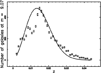
Figure 2: The galaxies of the 2MRS with $8.48\leq m\leq 10.44$ or $1202409\frac{L_{\ast{\odot}}}{Mpc^{2}}\leq f\leq 7267112\frac{L_{\ast{\odot}}}{Mpc^{2}}$ are organized in frequencies versus heliocentric redshift, (empty circles); the error bar is given by the square root of the frequency. The maximum frequency of observed galaxies is at $z=0.015$. The full line is the theoretical curve generated by $\frac{dN}{d\Omega dzdf}(z;z_{crit},c,H_{0})$. In this plot $M^{\odot}_{K_{S}}$ = 3.39, $h$ = 0.7, $M^{*}$=-24.87, $\alpha$ =-0.98, $\Phi^{*}$=0.0037, $\chi^{2}=721$ and the number of bins 40.

The total number of galaxies in the 2MRS as function of $z$ is reported in Figure 3 as well as the theoretical curve represented by the numerical integration of $\frac{dN}{d\Omega dzdf}(z;z_{crit},c,H_{0})$.

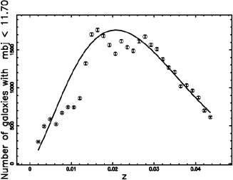
Figure 3: All the galaxies of the 2MRS with $m_{ks}<$ 11.75 are organized in frequencies versus heliocentric redshift, (empty circles); the error bar is given by the square root of the frequency. The maximum frequency of all observed galaxies is at $z=0.017$. The full line is the theoretical curve generated by $\frac{dN}{d\Omega dzdf}(z;z_{crit},c,H_{0})$. In this plot $M^{\odot}_{K_{S}}$ = 3.39, $h$ = 0.7, $M^{*}$=-23.97, $\alpha$ =-0.96, $\Phi^{*}$=0.0037, $\chi^{2}=1267$ and the number of bins is 30.

The mass of a galaxy can be evaluated once the mass luminosity ratio, $R$ is given by

$$R=\langle\frac{M}{L}\rangle\quad.$$ (3)

Some values of $R$ are now reported: $R\leq 20$ by Kiang (1961) and Persic & Salucci (1992), $R=20$ by Padmanabhan (1996) and $R=5.93$ by van der Marel (1991). The Malmquist bias, see Malmquist (1920, 1922), was originally applied to the stars and later on to the galaxies by Behr (1951). The observable absolute magnitude, $M_{L}(m_{L};z,H_{0})$, as a function of the limiting apparent magnitude, $m_{L}$, can be found in (Zaninetti, 2010b, Eqn. (51)). The bias predicts, from a theoretical point of view, an upper limit for the maximum absolute magnitude which can be observed in a catalog of galaxies characterized by a given limiting magnitude and Figure 4 reports such a curve as well the galaxies of the 2MRS.

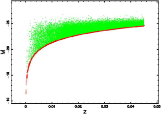
Figure 4: The absolute magnitude $M$ of 36464 galaxies belonging to the 2MRS when $M^{\odot}_{K_{S}}$ = 3.39 and $H_{0}=70\mathrm{\ km\ s}^{-1}\mathrm{\ Mpc}^{-1}$ (green points). The upper theoretical curve as represented by $M_{L}(m_{L};z,H_{0})$ is reported as the red thick line when $m_{L}$=11.75.

The limiting magnitude of the 2MRS is $m_{L}$=11.75 and therefore the 2MRS is complete for $z\leq 0.0025$. For values of $z$ greater than this value the observed sample is not complete and we can introduce the efficiency, $\epsilon_{s}(z;M_{max},M_{min},m_{L},c,h)$, where $M_{max}$ and $M_{min}$ are the maximum and minimum absolute magnitude of the considered catalog and $h=H_{0}/100$, see (Zaninetti, 2010b, Eqns. (51-53)). As an example when $z\approx 0.017$ the sample covers the 52$\%$ of the range in absolute magnitude.

4 The gravitational field

We now explore a connection with the shell theorem. Let us consider a spherically symmetric surface of radius $a$ on which a total mass $M$ is disposed in a uniform way. The mass per unit area $\mu$ is

$$\mu=\frac{M}{4\pi a^{2}}\quad.$$ (4)

The force at the internal of the spherical surface is

$$\Gamma=0\quad r<a\quad,$$ (5)

see Eq. (11.24) in Alonso & Finn (1992) and therefore the shell theorem can be formulated ”A uniform shell of matter exerts no gravitational force on a particle situated inside a shell”. We now compute the force on the center ($x$=0,$y$=0,$z$=0) of a hemisphere which resides on the positive z-axis. The vectorial intensity of the field is

$$d{\bf\Gamma}=G\frac{dm}{a^{2}}\quad,$$ (6)

being

$$dm=\mu a^{2}d\Omega\quad,$$ (7)

where $d\Omega=\sin\theta d\theta d\phi$ is the solid angle with $0\leq\phi\leq 2\pi$ and $0\leq\theta\leq\frac{\pi}{2}$. The three Cartesian components of the field in the 3D case are

$$\Gamma_{z}=\int_{0}^{2\pi}d\phi\,\int_{\frac{\pi}{2}}^{0}G\,\mu\,sin\theta\,cos\theta\,d\theta$$

$$\Gamma_{x}=\int_{0}^{2\pi}d\phi\,\int_{\frac{\pi}{2}}^{0}G\,\mu\,sin\theta\,sin\theta\,\cos\phi\,d\theta$$ (8)

$$\Gamma_{y}=\int_{0}^{2\pi}d\phi\,\int_{\frac{\pi}{2}}^{0}G\,\mu\,sin\theta\,sin\theta\,\sin\phi\,d\theta\quad.$$

The integration gives in the 3D case for the three forces at the center

$$\Gamma_{z}=\frac{GM}{2a^{2}}$$

$$\Gamma_{x}=\Gamma_{y}=0\quad.$$ (9)

We now consider the 2D case of mass concentrated on a half circle of radius $a$ situated on the positive $y$-axis, where now the mass per unit length $\mu_{2D}$ is

$$\mu_{2D}=\frac{M}{\pi a}\quad.$$ (10)

The 2D vectorial intensity of the field is

$$d{\bf\Gamma}=G\frac{dm}{a^{2}}\quad,$$ (11)

being

$$dm=\mu_{2D}ad\theta\quad,$$ (12)

where $0\leq\theta\leq\pi$. The 2D Cartesian gravitational components of the force at the center ($x$=0,$y$=0) are

$$\Gamma_{y}=G\frac{\mu_{2D}}{a}\int_{0}^{\pi}\sin\theta d\theta$$

$$\Gamma_{x}=G\frac{\mu_{2D}}{a}\int_{0}^{\pi}\cos\theta d\theta\quad.$$ (13)

The integration of the 2D case gives

$$\Gamma_{y}=\frac{2GM}{\pi a^{2}}$$

$$\Gamma_{x}=0\quad.$$ (14)

At the moment of writing the Committee on Data for Science and Technology (CODATA) recommends

$$G=(6.67384\pm 0.00080)\times 10^{-11}\frac{m^{3}}{kgs^{2}}\quad,$$ (15)

see Mohr et al. (2008). Before to continue we express the Newtonian gravitational constant in the following units: length in $Mpc$, mass in $M_{gal}$ which is $10^{11}M_{\ast{\odot}}$ and $yr8$ which are $10^{8}$ $yr$

$$G=4.4997510^{-6}\frac{Mpc^{3}}{M_{gal}yr8^{2}}\quad.$$ (16)

The two formulas (9) in 2D and (14) in 3D represent a useful reference to test a numerical code and to fix the range of variability of the gravitational field. According to our 3D theory the gravitational field at the center of the cosmic voids varies between the minimum value of zero (shell theorem) and a maximum value

$$\Gamma_{z}=\frac{GM}{2{\overline{R}}^{2}}=6.769\,10^{-9}N\,\,\frac{MpcM_{gal}}{yr8^{2}}\quad,$$ (17)

where $N$ is the number of galaxies in the spherical shell surrounding the cosmic void having mass $M=M_{gal}$ and ${\overline{R}}$=18.23 Mpc is the average radius of the cosmic voids.

We are now ready to process the 2MRS data and we associate to each galaxy, as reported in Figure 1 a mass given by Eqn. 3. The three components of the gravitational field are reported in table 3.

Table 3: 3D Gravitational forces expressed in $\frac{MpcM_{gal}}{yr8^{2}}$ at the center of a 3D box of side 37 $\times$ 2 Mpc when $R=$6 and theoretical 3D formula ( 9). At z=0.008 the efficiency of the sample is $\approx$ 70.6 $\%$.

$$\begin{array}[]{ccccc}\hline\cr\hline\cr\vskip 3.0pt plus 1.0pt minus 1.0pt\cr Environment&\Gamma_{x}&\Gamma_{y}&\Gamma_{z}&\|\Gamma\|\\ \vskip 3.0pt plus 1.0pt minus 1.0pt\cr\hline\cr\vskip 3.0pt plus 1.0pt minus 1.0pt\cr real~{}structure&-9.77\,10^{-6}&-1.53\,10^{-5}&-3.04\,10^{-6}&1.84\,10^{-5}\\ half~{}sphere&0&0&2.55\,10^{-5}&2.55\,10^{-5}\\ \vskip 3.0pt plus 1.0pt minus 1.0pt\cr\vskip 3.0pt plus 1.0pt minus 1.0pt\cr\hline\cr\hline\cr\end{array}$$

From a careful analysis of Table 3 it is possible to conclude that the gravitational field is greater than zero but smaller in respect to the case in which all the galaxies resides on a half sphere of radius equal to the averaged radius of the sample. Figure 5 reports a slice at the middle of a smaller box.

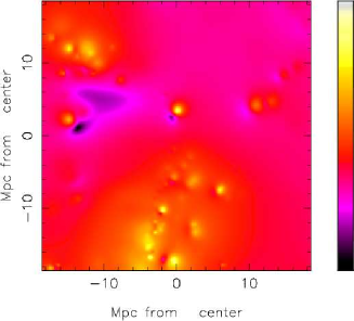
Figure 5: Cut-map of the 3D gravitational field of 2MRS when $R$=6. In order to have periodic boundary conditions the side of the box is 37 Mpc.

The spatial displacement of the 3D grid ${\Gamma}({i,j,k})$ which represent the absolute value of the gravitational field can be visualized through the iso-density contours, and as an example we considered a 101$\times$101$\times$101 grid. In order to do so, the maximum value ${\Gamma_{n}}({i,j,k)}_{max}$ and the minimum value ${\Gamma_{n}}({i,j,k)}_{min}$  should be extracted from the three-dimensional grid. A value of this grid can be fixed by the following equation:

$$\Gamma_{n}(i,j,k)_{chosen}=\Gamma_{n}(i,j,k)_{min}+(\Gamma_{n}(i,j,k)_{max}-\Gamma_{n}(i,j,k)_{min})\times{coef}\quad,$$ (18)

where coef is a parameter comprised between 0 and 1. This iso-surface rendering of the gravitational field is reported in Fig 6; the Euler angles characterizing the point of view of the observer are also reported.

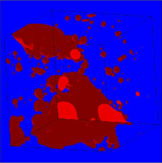
Figure 6: Iso–surface of the logarithm of the 3D gravitational field of 2MRS when $R$=6 and $coef=0.43$. The orientation of the figure is characterized by the Euler angles, which are $\Phi$=30^∘, $\Theta$=30^∘ and $\Psi$=30^∘.

Another interesting quantity to plot is the statistics of the values of the already defined spatial grid $\Gamma_{n}$ which holds 101 $\times$ 101 $\times$101 values of gravitational field, see Figure 7.

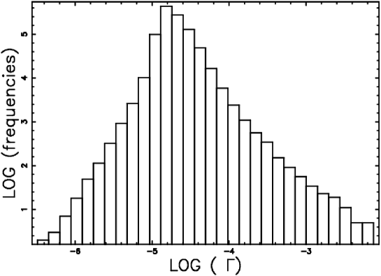
Figure 7: Decimal logarithmic histogram (step-diagram) of the values of the gravitational field evaluated in 101$\times$101$\times$101 points.

From this histogram is possible to conclude that the 90$\%$ of the space has a gravitational field comprised $3.24~{}10^{-7}\frac{MpcM_{gal}}{yr8^{2}}\leq\Gamma_{n}\leq 3.16~{}10^{-5}\frac{MpcM_{gal}}{yr8^{2}}$.

5 The Voronoi simulation

The Poisson Voronoi tessellation (PVT) is a useful tool to explore the spatial clustering of galaxies. The filaments of galaxies visible in the slices-type catalogs are due to the intersection between a plane and the PVT network of faces as a first approximation. An improvement can be obtained by coding the intersection between the slice of a given opening angle and the PVT network of faces, see Zaninetti (2006, 2010a). As an example Figure 8 reports both the CFA2 slice as well the simulated slice.

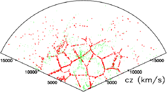
Figure 8: Polar plot of the real galaxies (green points) belonging to the second CFA2 redshift catalog and the simulated galaxies in the PVT framework (red points). More details can be found in Zaninetti (2006).

We now test formula (14) in a discrete environment rather than in the continuous case. The test now calculates the two forces $\Gamma_{x}$ and $\Gamma_{y}$ in the center of the circle and in a 2D irregular Voronoi polygon generated by PVT which has the same averaged radius of the circle and center occurring in the same location of the generating seed. The half Voronoi polygon and the half circle are displayed in Figure 9 and the two forces $\Gamma_{x}$ and $\Gamma_{y}$ in Table 4.

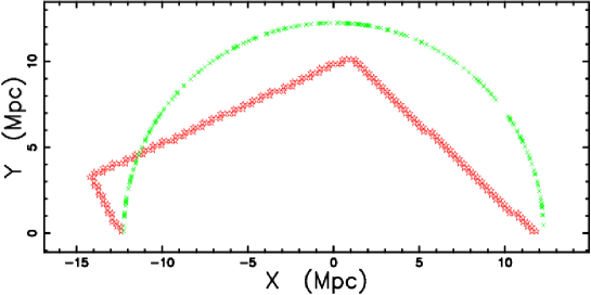
Figure 9: Half circle with $a$=12.25 Mpc (green stars) and half irregular polygon (red squares). The number of unit masses, 1 $M_{gal}$ is 455.

Table 4: Gravitational forces expressed in $\frac{MpcM_{gal}}{yr8^{2}}$ in the comparison between half circle, 2D formula (14), and half irregular polygon. The parameters are $M_{gal}$=455 and $a=12.25453Mpc$.

$$\begin{array}[]{ccc}\hline\cr\hline\cr\vskip 3.0pt plus 1.0pt minus 1.0pt\cr Environment&\Gamma_{x}&\Gamma_{y}\\ \vskip 3.0pt plus 1.0pt minus 1.0pt\cr\hline\cr\vskip 3.0pt plus 1.0pt minus 1.0pt\cr Half~{}circle-theory&0&8.67\,10^{-6}\\ Half~{}circle-numeric&-4.16\,10^{-8}&8.81\,10^{-6}\\ Half~{}polygon-numeric&1.37\,10^{-6}&1.36\,10^{-5}\\ \vskip 3.0pt plus 1.0pt minus 1.0pt\cr\vskip 3.0pt plus 1.0pt minus 1.0pt\cr\hline\cr\hline\cr\end{array}$$

We are now ready to process a real void and our attention is focused on a CFA2 slice visible in Figure 10.

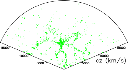
Figure 10: Polar plot of the real galaxies (green points) belonging to the second CFA2 redshift catalog.

A real void is extracted and the averaged radius of the galaxies on the boundary of that void is computed, see Figure 11.

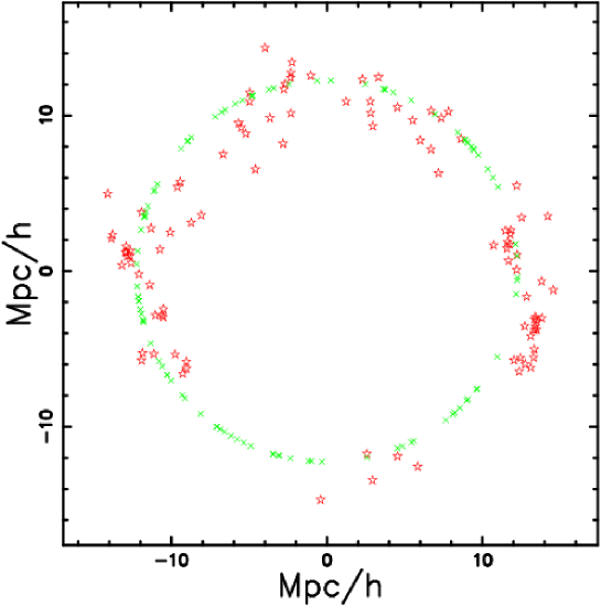
Figure 11: Circle with $a$= 12.25 Mpc (green stars) and real void extracted from a CFA2 slice (red squares). The number of galaxies with unit mass is 101.

The forces in the $x$ and $y$ direction are then computed and reported in Table 5.

Table 5: Gravitational forces expressed in $\frac{MpcM_{gal}}{yr8^{2}}$ for the comparison between a circle and a real CFA2 void. The parameters are $M_{gal}$=101 and $a=12.25453Mpc$.

$$\begin{array}[]{ccc}\hline\cr\hline\cr\vskip 3.0pt plus 1.0pt minus 1.0pt\cr Environment&\Gamma_{x}&\Gamma_{y}\\ \vskip 3.0pt plus 1.0pt minus 1.0pt\cr\hline\cr\vskip 3.0pt plus 1.0pt minus 1.0pt\cr circle--theory&0&0\\ half~{}circle--theory&0&1.92\,10^{-6}\\ real~{}void--numeric&-1.36\,10^{-7}&8.3\,10^{-7}\\ \vskip 3.0pt plus 1.0pt minus 1.0pt\cr\vskip 3.0pt plus 1.0pt minus 1.0pt\cr\hline\cr\hline\cr\end{array}$$

The presence of both a discrete number of galaxies and a non exactly symmetric displacement of the galaxies produces gravitational forces that take a finite value rather than zero. It is interesting to point out that $\Gamma_{y}$ due to the galaxies on the boundary of the real void is smaller than the theoretical value as given by the half circle which represents a maximum theoretical value.

6 Conclusions

The masses of the galaxies can be deduced starting from the luminosities in the framework of the mass luminosity ratio, $R$. The spatial distribution of the masses of the galaxies allows the computation of the Newtonian gravitational forces on the unit mass. As a reference for the evaluation of the forces the 2D and 3D shell theorem is analyzed. The evaluation of forces at the center of the box allows to conclude that the forces are smaller in respect to the mass concentrated on a half sphere of radius equal to the averaged radius of the selected sample of galaxies but bigger than zero due to the fact that the distribution of the galaxies is discrete rather than continuum. A careful analysis of a cubic box having side of 37 Mpc allows to say that the 90 $\%$ of the space has gravitational forces around the average value of $2.1\,10^{-5}\frac{MpcM_{gal}}{yr8^{2}}$.

References

- Abazajian et al. (2009) Abazajian, K. N., Adelman-McCarthy, J. K., Agüeros, M. A., Allam, S. S., Allende Prieto, C., An, D., Anderson, K. S. J., Anderson, S. F., Annis, J., Bahcall, N. A., & et al. 2009, ApJS , 182, 543
- Alonso & Finn (1992) Alonso, M., & Finn, E. 1992, Physics (New York: Addison-Wesley)
- Behr (1951) Behr, A. 1951, Astronomische Nachrichten, 279, 97
- Coil (2012) Coil, A. L. 2012, ArXiv:1202.6633
- Cole et al. (2001) Cole, S., Norberg, P., Baugh, C. M., Frenk, C. S., Bland-Hawthorn, J., Bridges, T., Cannon, R., Colless, M., Collins, C., Couch, W., Cross, N., Dalton, G., De Propris, R., Driver, S. P., Efstathiou, G., Ellis, R. S., Glazebrook, K., Jackson, C., Lahav, O., Lewis, I., Lumsden, S., Maddox, S., Madgwick, D., Peacock, J. A., Peterson, B. A., Sutherland, W., & Taylor, K. 2001, MNRAS , 326, 255
- Crook et al. (2007) Crook, A. C., Huchra, J. P., Martimbeau, N., Masters, K. L., Jarrett, T., & Macri, L. M. 2007, ApJ , 655, 790
- Huchra et al. (2012) Huchra, J. P., Macri, L. M., Masters, K. L., & et al. 2012, ApJS , 199, 26
- Jarrett (2004) Jarrett, T. 2004, PASA , 21, 396
- Kiang (1961) Kiang, T. 1961, MNRAS , 122, 263
- Malmquist (1920) Malmquist , K. 1920, Lund Medd. Ser. II, 22, 1
- Malmquist (1922) —. 1922, Lund Medd. Ser. I, 100, 1
- Mohr et al. (2008) Mohr, P. J., Taylor, B. N., & Newell, D. B. 2008, Journal of Physical and Chemical Reference Data, 37, 1187
- Padmanabhan (1996) Padmanabhan, T. 1996, Cosmology and Astrophysics through Problems (Cambridge: Cambridge University Press)
- Pan et al. (2011) Pan, D. C., Vogeley, M. S., Hoyle, F., Choi, Y.-Y., & Park, C. 2011, ArXiv e-prints:1103.4156
- Persic & Salucci (1992) Persic, M., & Salucci, P. 1992, MNRAS , 258, 14P
- Schechter (1976) Schechter, P. 1976, ApJ , 203, 297
- van der Marel (1991) van der Marel, R. P. 1991, MNRAS , 253, 710
- Zaninetti (2006) Zaninetti, L. 2006, Chinese J. Astron. Astrophys. , 6, 387
- Zaninetti (2010a) —. 2010a, Revista Mexicana de Astronomia y Astrofisica, 46, 115
- Zaninetti (2010b) —. 2010b, Serbian Astronomical Journal, 181, 19