Superlinear lower bounds for multipass graph processing

Abstract

We prove $n^{1+\Omega(1/p)}/p^{O(1)}$ lower bounds for the space complexity of $p$-pass streaming algorithms solving the following problems on $n$-vertex graphs:

• testing if an undirected graph has a perfect matching (this implies lower bounds for computing a maximum matching or even just the maximum matching size),

• testing if two specific vertices are at distance at most $2(p+1)$ in an undirected graph,

• testing if there is a directed path from $s$ to $t$ for two specific vertices $s$ and $t$ in a directed graph.

The lower bounds hold for $p=O(\log n/\log\log n)$. Prior to our result, it was known that these problems require $\Omega(n^{2})$ space in one pass, but no $n^{1+\Omega(1)}$ lower bound was known for any $p\geq 2$.

These streaming results follow from a communication complexity lower bound for a communication game in which the players hold two graphs on the same set of vertices. The task of the players is to find out whether the sets of vertices at distance exactly $p+1$ from a specific vertex intersect. The game requires a significant amount of communication only if the players are forced to speak in a specific difficult order. This is reminiscent of lower bounds for communication problems such as indexing and pointer chasing. Among other things, our line of attack requires proving an information cost lower bound for a decision version of the classic pointer chasing problem and a direct sum type theorem for the disjunction of several instances of this problem.

1 Introduction

Graph problems in the streaming model have attracted a fair amount of attention over the last 15 years. Formally, a streaming algorithm is presented with a sequence of graph edges and it can read them one by one in the order in which they appear in the sequence. The main computational resource studied for this kind of algorithm is the amount of space it can use, i.e., the amount of information about the graph the algorithm remembers during its execution.

Due to advances in the storage technology, it is feasible nowadays to collect large amounts of data. Companies store more and more information for reasons that include data mining applications and legal obligations. Sequential access often maximizes readout efficiency in the case of external storage devices. Whenever a single-pass streaming algorithm requires an infeasible amount of main memory, it is natural to ask whether there exists a significantly more efficient algorithm that uses a very small number of passes over data.

At a more theoretical level, relations between nodes (i.e., how they are connected in the graph and what the distances between them are) are a fundamental property of graphs that is worth studying. When it comes to exploring the structure of graphs, allowing for multiple passes seems to greatly improve the capabilities of streaming algorithms. For instance, the algorithm of Das Sarma, Gollapudi, and Panigrahy [11], which received the best paper award at PODS 2008, uses multiple passes to construct long random walks in the graph in order to approximate PageRank for vertices. Also many strong lower bounds of $\Omega(n^{2})$ space for one pass easily break if more than one pass is allowed. This is for instance the case for the early lower bounds of Henzinger, Raghavan, Rajogopalan [21] and also the lower bounds of Feigenbaum et al. [15].

On the other hand, constructing lower bounds for graph problems is usually based on constructing obstacles for local exploration, and our paper is not different in this respect. We show that finding out if two vertices are at a specific small distance $p$ essentially requires $p/2$ passes to be accomplished in space $O(n)$. The main idea is similar to what is done for pointer chasing. Namely, we place edges in the order opposite to the sequence which enables easy exploration.

Our results. Let $n$ be the number of vertices in the graph and let $p$ be the allowed number of passes. We show strongly superlinear lower bounds of $T_{n,p}=\Omega\left(\frac{n^{1+1/(2p+2)}}{p^{20}\log^{3/2}n}\right)$ bits of space for three problems:

• testing if the graph has a perfect matching,

• testing if two prespecified vertices $u$ and $v$ are at distance at most $2(p+1)$ for an undirected input graph,

• testing if there is a directed path from $u$ to $v$, where $u$ and $v$ are prespecified vertices and the input graph is directed.

In general, lower bounds stronger than $\Omega(n)$ require embedding a difficult instance of a problem into the “space of edges” as opposed to the “space of vertices,” which turns out to be difficult in many cases. For instance, the $\Omega(n^{2})$ lower bounds of [21] and [15] do not hold for algorithms that are allowed more than one pass.

Communication complexity is a standard tool for proving streaming lower bounds. We describe our hard communication problem from which we reduce to the streaming problems in Section 2. We now overview related work.

Matchings. In the maximum matching problem, the goal is to produce a maximum-cardinality set of non-adjacent edges. Streaming algorithms for this problem and its weighted version have received a lot of attention in recent years [15, 28, 13, 1, 27, 17, 25, 14, 34].

Our result compares most directly to the lower bound of Feigenbaum et al. [15], who show that even checking if a given matching is of maximum size requires $\Omega(n^{2})$ space in one pass. Our result can be seen as an extension of their lower bound to the case when multiple passes are allowed. Even when $p\geq 2$ passes are allowed, we show that still a superlinear amount of space, roughly $n^{1+\Omega(1/p)}$, is required to find out if there is a perfect matching in the graph. This of course implies that tasks such as computing a maximum matching or even simply the size of the maximum matching also require this amount of space.

For the approximate version of the maximum matching problem, McGregor [28] showed that a $(1-\varepsilon)$-approximation can be computed in $\tilde{O}(n)$ space with the number of passes that is a function of only $\varepsilon$. The only known superlinear lower bound for the approximate matching size applies only to one-pass algorithms and shows that the required amount of space is $n^{1+\Omega(1/\log\log n)}$ if a constant approximation factor better than $1-e^{-1}$ is desired [17, 25].

Shortest paths. We now move to the problem of computing distances between vertices in an undirected graph. Feigenbaum et al. [16] show that $\tilde{O}(n)$ space and one pass suffice to compute an $O(\log n/\log\log n)$-spanner and therefore approximate all distances up to a factor of $O(\log n/\log\log n)$. They also show a closely matching lower bound of $\Omega(n^{1+1/t})$ for computing a factor $t$ approximation to distances between all pairs of vertices.

In the result most closely related to ours, they show that computing the set of vertices at distance $p$ from a prespecified vertex in less than $p/2$ passes requires $n^{1+\Omega(1/p)}$ space. One can improve their lower bound to show that it holds even when the number of allowed passes is $p-1$. As a result, to compute the distance $p$ neighborhood in $O(n)$ space, essentially the best thing one can do is to simulate the BFS exploration with one step per pass over the input, which requires $p$ passes. In this paper, we show a similar lower bound for the problem of just checking if two specific vertices are at distance exactly $p$. Our problem is algorithmically easier. If two vertices are at distance $p$, $\lceil p/2\rceil$ passes and $O(n)$ space suffice, because one can simulate the BFS algorithm up to the radius of $\lceil p/2\rceil$ from both vertices of interest. This is one of the reasons why our result cannot be shown directly by applying their lower bound.

A space lower bound of $\Omega(n^{2})$ for one pass algorithms to find whether a pair of nodes is at distance $3$ can be found in [15].

Directed connectivity. Feigenbaum et al. [15] show that the directed $u$-$v$ connectivity problem requires $\Omega(n^{2})$ bits of space to solve in one pass. However, their lower bound does not extend to more than one pass. Once again our lower bound extends their result to show that a superlinear lower bound holds for multiple passes. (Note that for undirected graphs, the problem of connectivity can easily be solved with one pass and $\tilde{O}(n)$ space, using for instance the well known union-find algorithm.)

Optimality of our lower bound. We conjecture that our lower bounds can be improved from $\tilde{\Omega}(n^{1+1/(2p+2)})$ to $\tilde{\Omega}(n^{1+1/(p+1)})$ for $p=O(1)$. For the matching problem, our lower bound is based on showing that finding a single augmenting path is difficult. It is an interesting question if a stronger lower bound can be proved in the case where more augmenting paths have to be found. Currently, no $o(n^{2})$-space streaming algorithm is known for this problem with a small number of passes.

Paper organization. We begin in Section 2 with a description of the communication problems we study and a high-level overview of our lower bound approach. We set up some useful information-theoretic preliminaries in Section 3. We state our main communication complexity lower bound (Theorem 4) and use it to show our streaming lower bounds in Section 4. Our communication lower bound is proved in three steps, and we go into the details of these steps in the next three sections. Finally, in Section 8 we put the steps together to give a proof of Theorem 4.

2 Proof overview and techniques

Via simple reductions, our multipass streaming lower bounds for matching and connectivity reduce to proving communication complexity lower bounds for a certain decision version of “set pointer chasing.” The reductions to streaming are described in Section 4. In the current section we give an overview of our communication complexity results. We start with a quick review of information and communication complexity and then introduce communication problems that are useful in our proof.

We assume private randomness in all communication problems, unless otherwise stated. Furthermore, all messages are public, i.e., can be seen by all players (the setting sometimes described as the blackboard model).

2.1 Information and Communication Complexity

Communication complexity and information complexity play an important role in our proofs. We now provide necessary definitions for completeness.

The communication complexity of a protocol is the function from the input size to the maximum length of messages generated by the protocol on an input of a specific size. For a problem $\mathcal{X}$ and $\delta\in[0,1]$, the communication complexity of $\mathcal{X}$ with error $\delta$ is the function from the input size to the infimum communication complexity of private-randomness protocols that err with probability at most $\delta$ on any input. We write $R_{\delta}(\mathcal{X})$ to denote this quantity.

The information cost $\operatorname{ICost}_{\psi}(\Pi)$ of a protocol $\Pi$ on input distribution $\psi$ equals the mutual information $I(X;\Pi(X))$, where $X$ is the input distributed according to $\psi$ and $\Pi(X)$ is the transcript of $\Pi$ on input $X$.

The information complexity $\operatorname{IC}_{\psi,\delta}$ of a problem $\mathcal{X}$ on a distribution $\psi$ with error $\delta$ is the infimum $\operatorname{ICost}_{\psi}(\Pi)$ taken over all private-randomness protocols $\Pi$ that err with probability at most $\delta$ for any input.

2.2 Communication Problems

Consider a communication problem with $p$ players $P_{1}$, …, $P_{p}$. Players speak in $r$ rounds and in each round they speak in order $P_{1}$ through $P_{p}$. At the end of the last round, the player $P_{p}$ has to output the solution. We call any such problem a $(p,r)$-communication problem.

We define $[n]$ as $\{1,\ldots,n\}$. For any set $A$, we write $2^{A}$ to denote the power set of $A$, i.e., the set of all subsets of $A$. For any function $f:A\to 2^{B}$, we define a mapping $\vv{f}:2^{A}\to 2^{B}$ such that $\vv{f}(S)=\bigcup_{s\in S}f(s)$.

Pointer and Set Chasing. The pointer chasing communication problem $\mbox{\sf PC}_{n,p}$, where $n$ and $p$ are positive integers, is a $(p,p-1)$-communication problem in which the $i$-th player $P_{i}$ has a function $f_{i}:[n]\to[n]$ and the goal is to compute $f_{1}(f_{2}(\ldots f_{p}(1)\ldots))$. The complexity of different versions of this problem was explored thoroughly by a number of works [31, 12, 30, 10, 32, 7, 18, 19].

The set chasing communication problem $\mbox{\sf SC}_{n,p}$, for given positive integers $n$ and $p$, is a $(p,p-1)$-communication problem in which the $i$-th player $P_{i}$ has a function $f_{i}:[n]\to 2^{[n]}$ and the goal is to compute $\vv{f_{1}}(\vv{f_{2}}(\ldots\vv{f_{p}}(\{1\})\ldots))$. A two-player version of the problem was considered by Feigenbaum et al. [16].

Operators on Problems. For a $(p,r)$-communication problem $\mathcal{X}$, we write $\operatorname{\mbox{\sf EQUAL}}(\mathcal{X})$ to denote a $(2p,r)$-communication problem in which the first $p$ players $P_{1}$, …, $P_{p}$ hold one instance of $\mathcal{X}$, the next $p$ players $P_{p+1}$, …, $P_{2p}$ hold another instance of $\mathcal{X}$, and the goal is to output one bit that equals $1$ if and only if the outputs for the instances of $\mathcal{X}$ are equal. See Figure 1 for an example.

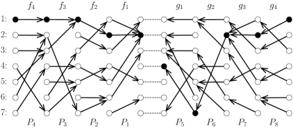
Figure 1: A sample instance of $\operatorname{\mbox{\sf EQUAL}}(\mbox{\sf PC}_{7,4})$ with a negative solution. It consists of two instances of $\mbox{\sf PC}_{7,4}$ held by two different sets of players.

Analogously, for a $(p,r)$-communication problem $\mathcal{X}$ such that the output is a set, we write $\operatorname{\mbox{\sf INTERSECT}}(\mathcal{X})$ to denote the $(2p,r)$-communication problem in which the first $p$ players $P_{1}$, …, $P_{p}$ hold one instance of $\mathcal{X}$, the next $p$ players $P_{p+1}$, …, $P_{2p}$ hold another instance of $\mathcal{X}$, and the goal is to output one bit that equals $1$ if and only if the sets that are solutions to the instances of $\mathcal{X}$ intersect. See Figure 2 for an example.

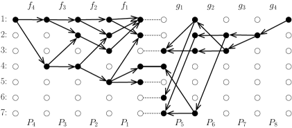
Figure 2: A sample instance of $\operatorname{\mbox{\sf INTERSECT}}(\mbox{\sf SC}_{7,4})$, where two final sets intersect. The edges outgoing from vertices that are not visited were omitted.

For a $(p,r)$-communication problem $\mathcal{X}$ with a Boolean output, we write $\operatorname{\mbox{\sf OR}}_{t}(\mathcal{X})$, where $t$ is a positive integer, to denote the $(p,r)$-communication problem in which players have $t$ instances of $\mathcal{X}$ and want to output the disjunction of their results.

Limited Pointer Chasing Equality. We say that a function $f:A\to B$ is $t$-colliding, where $t$ is a positive integer, if there is an $A^{\prime}\subseteq A$ of size $t$ and a $b\in B$ such that for all $a\in A^{\prime}$, $f(a)=b$.

We write ${\mbox{\sf LPCE}_{n,k,t}}$ to denote a modified version of $\operatorname{\mbox{\sf EQUAL}}(\mbox{\sf PC}_{n,k})$. In ${\mbox{\sf LPCE}_{n,k,t}}$ the last player has to output the same value as in $\operatorname{\mbox{\sf EQUAL}}(\mbox{\sf PC}_{n,k})$, unless one of the functions in one of the pointer chasing instances is $t$-colliding, in which case the last player has to output $1$. This is a technical extension to ensure that no element has too many pre-images, which is necessary to make one of our reductions work.

2.3 Lower bound for $\operatorname{\mbox{\sf INTERSECT}}(\mbox{\sf SC}_{n,p})$

Our multipass streaming lower bounds for matching and connectivity reduce to proving a communication complexity lower bound for the set chasing intersection problem $\operatorname{\mbox{\sf INTERSECT}}(\mbox{\sf SC}_{n,p})$. Note that if the players spoke in the order $P_{2p}$, $P_{2p-1}$, …, $P_{1}$, then they would be able to solve both instances of $\mbox{\sf SC}_{n,p}$, using at most $O(n)$ communication per player, which is enough to solve the intersection problem. If the players spoke in the desired order $P_{1}$, $P_{2}$, …, $P_{2p}$ but were allowed a total of $p$ rounds then they would be able to solve the instances of $\mbox{\sf SC}_{n,p}$ with $O(n)$ communication per message by simulating one step in the pointer chasing instance per round. Our main result is however that if the number of allowed rounds is $p-1$, then approximately $n^{1+\Omega(1/p)}$ bits of communication are needed to solve the problem, even for randomized protocols with constant error.

Our result is reminiscent of the classic $\Omega(n)$ communication complexity lower bounds for problems such as indexing and pointer chasing $\mbox{\sf PC}_{n,p}$ [30, 19] when the players speak in the “wrong” order. Guha and McGregor [19] adapt the proof of Nisan and Wigderson [30] to show that solving $\mbox{\sf PC}_{n,p}$ (in $p-1$ passes) requires $\Omega(n)/p^{O(1)}$ total communication even if the protocol can be randomized and can err with small constant probability. Increasing the number of rounds to $p$ or letting the players speak in the opposite order (even in just one round) would result in a problem easily solvable with messages of length $O(\log n)$.

Even more directly related is the construction of Feigenbaum et al. [16], who show that solving $\mbox{\sf SC}_{n,p}$ requires $n^{1+\Omega(1/p)}$ communication in less then $p$ passes. Their proof follows by using a direct sum theorem of Jain, Radhakrishnan and Sen [24] to show that solving $t\approx n^{\Theta(1/p)}$ instances of $\mbox{\sf PC}_{n,p}$ requires roughly $t$ times more communication than solving a single instance. Then they show that an efficient protocol for solving $\mbox{\sf SC}_{n,p}$ would result in an efficient protocol for solving $t$ instances of $\mbox{\sf PC}_{n,p}$ in parallel.

Compared to $\mbox{\sf SC}_{n,p}$, $\operatorname{\mbox{\sf INTERSECT}}(\mbox{\sf SC}_{n,p})$ is a decision problem. In particular, there seems to be no reduction allowing one to reconstruct the sets reached in $\operatorname{\mbox{\sf INTERSECT}}(\mbox{\sf SC}_{n,p})$. The only thing that we learn after an execution of the protocol is whether these two sets intersect. Therefore, reducing our question to that of [16] seems unlikely.

Our proof of the above communication complexity lower bound proceeds in three steps:

 Step A:

Reduction to proving a communication lower bound for $\operatorname{\mbox{\sf OR}}_{t}(\operatorname{\mbox{\sf EQUAL}}(\mbox{\sf PC}_{n,p}))$.

 Step B:

A direct sum style step lower bounding the communication complexity of $\operatorname{\mbox{\sf OR}}_{t}(\operatorname{\mbox{\sf EQUAL}}(\mbox{\sf PC}_{n,p}))$ as roughly $t$ times the information complexity of $\operatorname{\mbox{\sf EQUAL}}(\mbox{\sf PC}_{n,p})$.

 Step C:

An information complexity lower bound for $\operatorname{\mbox{\sf EQUAL}}(\mbox{\sf PC}_{n,p})$.

The technical body of the paper actually proves these steps in the opposite order (Steps A, B, and C are discussed in Sections 7, 6, and 5, respectively). But here we will expand on the steps in the above order. The actual proof works with a variant of $\operatorname{\mbox{\sf EQUAL}}(\mbox{\sf PC}_{n,p})$, namely $\mbox{\sf LPCE}_{n,p,r}$, which we defined earlier, in order to deal with functions $f_{i}$ that may be highly colliding, and which may break the reduction in Step A. For simplicity, we ignore this aspect in the overview, but it is worth keeping in mind that this complicates the execution of Step C on the information complexity lower bound.

Step A: Reduction to proving a lower bound for $\operatorname{\mbox{\sf OR}}_{t}(\operatorname{\mbox{\sf EQUAL}}(\mbox{\sf PC}_{n,p}))$. Our idea here is to use a communication protocol for $\operatorname{\mbox{\sf INTERSECT}}(\mbox{\sf SC}_{n,p})$ to give a protocol that can answer if at least one of the $t$ instances of $\operatorname{\mbox{\sf EQUAL}}(\mbox{\sf PC}_{n,p})$ has a Yes answer, where $t=n^{\Theta(1/p)}$. (Recall that in the $\operatorname{\mbox{\sf EQUAL}}(\mbox{\sf PC}_{n,p})$ problem, the input consists of two instances of $\mbox{\sf PC}_{n,p}$ with functions $\{f_{i},g_{i}:[n]\to[n]\}_{i=1}^{p}$ and the goal is to output Yes iff we end up at the same index in both instances, i.e., if $f_{1}(f_{2}(\ldots f_{p}(1)\ldots))=g_{1}(g_{2}(\ldots g_{p}(1)\ldots))$.) Given $t$ instances of $\operatorname{\mbox{\sf EQUAL}}(\mbox{\sf PC}_{n,p})$, for each instance independently, we randomly scramble the connections in every layer while preserving the answer to $\operatorname{\mbox{\sf EQUAL}}(\mbox{\sf PC}_{n,p})$. We then overlay all these instances on top of each other to construct an instance of $\operatorname{\mbox{\sf INTERSECT}}(\mbox{\sf SC}_{n,p})$ (note that each node has exactly $t$ neighbors in the next layer).

By construction, given a Yes instance of $\operatorname{\mbox{\sf OR}}_{t}(\operatorname{\mbox{\sf EQUAL}}(\mbox{\sf PC}_{n,p}))$, by following the mappings from the instance of $\operatorname{\mbox{\sf EQUAL}}(\mbox{\sf PC}_{n,p})$ which has a Yes answer, we also obtain an element that belongs to the intersection of the two resulting sets in $\operatorname{\mbox{\sf INTERSECT}}(\mbox{\sf SC}_{n,p})$. Since $t=n^{\Theta(1/p)}$, we have $t^{2p}\ll n$, and we argue that the random scramblings ensure that if none of $t$ instances of $\operatorname{\mbox{\sf EQUAL}}(\mbox{\sf PC}_{n,p})$ have a Yes answer, then it is unlikely that the two resulting sets in the instance of $\operatorname{\mbox{\sf INTERSECT}}(\mbox{\sf SC}_{n,p})$ will intersect. This constraint on $t$ is what limits our lower bound to ${\sim}\,n^{1+1/(2p)}$.

Step B: A direct sum style argument. In this step, our goal is to argue that the randomized communication complexity of $\operatorname{\mbox{\sf OR}}_{t}(\operatorname{\mbox{\sf EQUAL}}(\mbox{\sf PC}_{n,p}))$ is asymptotically $\Omega(t)$ times larger than that of $\operatorname{\mbox{\sf EQUAL}}(\mbox{\sf PC}_{n,p})$. This is reminiscent of direct sum results of the flavor that computing answers to $t$ instances of a problem requires asymptotically $t$ times the resources, but here we only have to compute the OR of $t$ instances. Our approach is to use the information complexity method that has emerged in the last decade as a potent tool to tackle such direct sum like questions [9, 2, 24], and more recently in [3, 5] and follow-up works. The introductions of [3, 22] contain more detailed information and references on direct sum and direct product theorems in communication complexity.

Our hard distribution will be the uniform distribution over all inputs. Being a product distribution, the information complexity will be at least the sum of the mutual information between the $i$-th input and the transcript, for $1\leq i\leq t$. Using the fact that the probability of a Yes answer on a random instance of $\operatorname{\mbox{\sf EQUAL}}(\mbox{\sf PC}_{n,p})$ is very small (at most $O(1/n)$), we prove that the mutual information between the $i$-th input and the transcript cannot be much smaller than the information cost of $\operatorname{\mbox{\sf EQUAL}}(\mbox{\sf PC}_{n,p})$ for protocols that err with probability $o(1/n)$ under the uniform distribution.

Step C: Lower bound for information cost of $\operatorname{\mbox{\sf EQUAL}}(\mbox{\sf PC}_{n,p})$. This leaves us with the task of lower bounding the information cost of low error protocols for $\operatorname{\mbox{\sf EQUAL}}(\mbox{\sf PC}_{n,p})$ under the uniform distribution. This is the most technical of the three steps. We divide this step into two parts.

First we show that if there were a protocol with low information cost $\operatorname{IC}$ on the uniform distribution, then there would exist a deterministic protocol that on the uniform distribution would send mostly short messages and err with at most twice the probability. This is done by adapting the proof of the message compression result of [24] for bounded round communication protocols. We cannot use their result as such since in order to limit the increase in error probability to $\gamma$, the protocol needs to communicate $\Omega(1/\gamma^{2})$ bits. This is prohibitive for us as we need to keep the error probability as small as $O(1/n)$, and can thus only afford an additive $O(1/n)$ increase. We present a twist to the simulation obtaining a deterministic protocol with at most twice the original error probability. The protocol may send a long message with some small probability $\varepsilon$ and in other cases communicates at most $O(\operatorname{IC}/\varepsilon^{2})$ bits. In our application, we set $\varepsilon$ to be a polynomial in $1/p$.

The second part is a lower bound for $\operatorname{\mbox{\sf EQUAL}}(\mbox{\sf PC}_{n,p})$ against such “typically concise” deterministic protocols. To prove this, we show that if the messages in the deterministic protocol are too short, then with probability at least $1/2$, the protocol will have little knowledge about whether the solutions to two instances of pointer chasing are identical and therefore, will still err with probability $\Omega(1/n)$, which is significant from our point of view. The proof extends the lower bound for pointer chasing due to Nisan and Wigderson [30] and its adaptation due to Guha and McGregor [19]. We have to overcome some technical hurdles as we need a lower bound for the equality checking version and not for the harder problem of computing the pointer’s value. Further, we need to show that a constant fraction of the protocol leaves are highly uncertain about their estimate of the pointers’ values, so that they would err with probability $\Omega(1/n)$ (with $1/n$ being the collision probability for completely random and independent values).

Summarizing, Step C can be seen as a modification of techniques of [30, 19] to prove a communication lower bound for $\operatorname{\mbox{\sf EQUAL}}(\mbox{\sf PC}_{n,p})$ combined with techniques borrowed from [24] to imply a lower bound for information complexity. The relationship between information complexity and communication complexity has been a topic of several papers, starting with [9, 24] for protocols with few rounds, and more recently [3, 5, 4, 8, 6, 26] for general protocols.

3 Preliminaries

Constant $C_{\star}$. Let $C_{\star}$ be a constant such that the probability that a function $f:[n]\to[n]$ selected uniformly at random is $C_{\star}(1+\log n)$-colliding is bounded by $1/(2n^{2})$. The existence of $C_{\star}$ follows from a combination of the Chernoff and union bounds.

3.1 Useful information-theoretic lemmas

Let us first recall a result that says that if a random variable has large entropy, then it behaves almost like the uniform random variable on large sets.

Fact 1 ([33], see also [30, Lemma 2.10]).

Let $X$ be a random variable on $[n]$ with $H(X)\geq\log n-\delta$. Let $S\subseteq[n]$ and let $\Delta=\sqrt{\frac{4\delta n}{|S|}}$. If $\Delta\leq 1/10$, then $\Pr[X\in S]\geq\frac{|S|}{n}\left(1-\Delta\right).$

Using the above result, we show that it is hard to guess correctly with probability $1-o(1/n)$ if two independent random variables distributed on $[n]$ collide if they have large entropy.

Lemma 2.

Let $X$ and $Y$ be two independent random variables distributed on $[n]$ such that both $H(X)$ and $H(Y)$ are at least $\log n-\delta$, where $\delta=48^{-2}$. Then

• $\Pr[X=Y]\geq 1/(8n)$, and

• if $n\geq 4$, $\Pr[X\neq Y]\geq 1/4$.

Proof.

We first prove that there is a set $S_{X}\subseteq[n]$ such that $|S_{X}|\geq\frac{3}{4}n$ and for each $x\in S_{X}$, $\Pr[X=x]\geq 1/(2n)$. Suppose that there is no such set. Then there is a set $T_{X}$ of size more than $n/4$ in which every element has probability strictly less than $1/(2n)$, and therefore, $\Pr[X\in T_{X}]<\frac{|T_{X}|}{2n}$. Note that $\sqrt{\frac{4\delta n}{|T_{X}|}}\leq 1/12<1/10$, which implies that we can apply Fact 1 to $T_{X}$. We obtain $\Pr[X\in T_{X}]\geq\frac{11}{12}\cdot\frac{|T_{X}|}{n}$, which contradicts the size of $T_{X}$ and implies that $S_{X}$ with the desired properties does exist.

Analogously, one can prove that there is a set $S_{Y}\subseteq[n]$ such that $|S_{Y}|\geq\frac{3}{4}n$ and for each $y\in S_{Y}$, $\Pr[Y=y]\geq 1/(2n)$. Note that $|S_{X}\cap S_{Y}|\geq n/2$. For each $x\in S_{X}\cap S_{Y}$, $\Pr[X=Y=x]\geq 1/(4n^{2})$. Hence

$$\Pr[X=Y]\geq\sum_{x\in S_{X}\cap S_{Y}}\Pr[X=Y=x]\geq 1/(8n).$$

To prove the second claim, for $n\geq 4$, observe that for every setting $x$ of $X$, $|S_{y}\setminus\{x\}|\geq\frac{3n}{4}-1\geq n/2$, and therefore, the probability that $Y\neq X$ is at least $|S_{y}\setminus\{x\}|\cdot 1/(2n)\geq 1/4$.∎

The following lemma gives a bound on the entropy of a variable that randomly selects out of two random values based on another $0$-$1$ valued random variable. We present a simple proof suggested by an anonymous reviewer.

Lemma 3.

Let $X_{0}$, $X_{1}$, and $Y$ be independent discrete random variables, where $X_{0}$ and $X_{1}$ are distributed on the same set $\Omega$ and $Y$ is distributed on $\{0,1\}$. Then

$$H(X_{Y})\leq 1+\sum_{i=0}^{1}\Pr[Y=i]\cdot H(X_{i}).$$

Proof.

It follows from basic properties of entropy that

$$H(X_{Y}) \leq H(Y;X_{Y})=H(Y)+H(X_{Y}|Y)$$

$$\leq 1+H(X_{Y}|Y)=1+\sum_{i=0}^{1}\Pr[Y=i]\cdot H(X_{i}).$$

∎

4 The Main Tool and Its Applications

The main tool in our paper is the following lower bound for the communication complexity of set chasing intersection.

Theorem 4.

For $n$ larger than some positive constant and $p$ such that $1<p\leq\frac{\log n}{\log\log n}$,

$$R_{1/10}(\operatorname{\mbox{\sf INTERSECT}}(\mbox{\sf SC}_{n,p}))=\Omega\left(\frac{n^{1+1/(2p)}}{p^{16}\cdot\log^{3/2}n}\right).$$

We now present relatively straightforward applications of this theorem to three graph problems in the streaming model.

Theorem 5.

Solving the following problems with probability at least $9/10$ in the streaming model with $p=O\left(\frac{\log n}{\log\log n}\right)$ passes requires at least $\Omega\left(\frac{n^{1+1/(2(p+1))}}{p^{19}\cdot\log^{3/2}n}\right)$ bits of space:

 Problem 1:

For two given vertices $u$ and $v$ in an undirected graph, check if the distance between them is at most $2(p+1)$.

 Problem 2:

For two given vertices $u$ and $v$ in a directed graph, check if there is a directed path from $u$ to $v$.

 Problem 3:

Test if the input graph has a perfect matching.

Proof.

Let us consider the problems one by one. For Problem 1, we turn an instance of $\operatorname{\mbox{\sf INTERSECT}}(\mbox{\sf SC}_{k,p+1})$ into a graph on $n=(2p+3)\cdot k$ vertices. We modify the graph in Figure 2 as follows. First, we make all edges undirected. Second, we merge every pair of middle vertices connected with a horizontal line into a single vertex. Any path between the top leftmost vertex $u$ and the top rightmost vertex $v$ is of length at least $2p+2$. The length of the path is exactly $2p+2$ if and only if it moves to the next layer in each step. Note that this corresponds to the case that the final sets for two instances of $\mbox{\sf SC}_{k,p+1}$ intersect. We create the input stream by inserting first the edges describing the function held by $P_{1}$, then by $P_{2}$ and so on, until $P_{2p+2}$. If there is a streaming algorithm for the problem that uses at most $T$ bits of space, then clearly there is a communication protocol for $\operatorname{\mbox{\sf INTERSECT}}(\mbox{\sf SC}_{k,p+1})$ with total communication $(2p+2)\cdot p\cdot T$ and the same error probability as the streaming algorithm. The protocol can be obtained by the players by simulating the streaming algorithms on their parts of the input and communicating its state. This implies that $T=\Omega\left(\frac{1}{p^{2}}\cdot\frac{(n/p)^{1+1/(2(p+1))}}{p^{16}\cdot\log^{3/2}n}\right)=\Omega\left(\frac{n^{1+1/(2(p+1))}}{p^{19}\cdot\log^{3/2}n}\right)$, where we use the fact that $p^{1/(2(p+1))}=O(1)$.

For Problem 2, the reduction is almost the same, with the only difference being that we make all edges directed from left to right and we want to figure out if there is a directed path from the top leftmost vertex to the top rightmost vertex. Such a path exists if and only if the final sets in the instance of $\operatorname{\mbox{\sf INTERSECT}}(\mbox{\sf SC}_{k,p+1})$ intersect.

Figure 3: Reduction to the perfect matching problem.

For Problem 3, the reduction is slightly more complicated. We show how to modify the hard instance $G$ that we have created for Problem 1. Let us first add a perfect matching before and after every layer of edges of the hard instance for Problem 1, except for the first and the last layer, in which we omit one edge. The omitted edges are incident to the vertices $u$ and $v$ corresponding to value 1, i.e., the vertices that we want to connect using a path going directly from left to right in Problem 1. See Figure 3 for an example. Note that the additional edges constitute a matching $M$ in which all but two vertices are matched. Now the graph has a perfect matching iff there exists an augmenting path in $M$ between $u$ and $v$, which are the unmatched vertices. Any augmenting path has to alternate between matched and unmatched edges, which implies in our case, that it has to go directly from left to right. Therefore, any augmenting path in $M$ corresponds to a path going directly from left to right in $G$ and connecting $u$ and $v$. The only difference is that the augmenting path has additional edges coming from the matchings that were inserted into $G$. Therefore the streaming algorithm for testing if a graph has a perfect matching can be used to create a protocol for $\operatorname{\mbox{\sf INTERSECT}}(\mbox{\sf SC}_{k,p+1})$, which requires relabeling endpoints of some edges—in order to simulate splitting of vertices—and inserting additional edges at the end of the stream. ∎

5 Step 1: Information Complexity of Pointer Chasing Equality

To prove the main theorem of the paper, we first show a lower bound for the information complexity of Limited Pointer Chasing Equality.

Lemma 6.

Let $n$ and $p$ be positive integers such that $n\geq 30p^{2}$ and $p>1$. Then

$$\operatorname{IC}_{\mu,1/(64n)}(\mbox{\sf LPCE}_{n,p,C_{\star}(1+\log n)}) \geq\frac{n}{2^{29}\cdot 3^{5}\cdot p^{16}}-\frac{\lceil 2\log n\rceil}{2^{13}\cdot 3^{2}\cdot p^{8}}-2$$

$$=\Omega\left(\frac{n}{p^{16}}\right)-O\left(\frac{\log n}{p^{8}}+1\right),$$

where $\mu$ is the uniform distribution on all possible inputs for the problem.

The proof consists of two smaller steps. First we show that if there is a protocol with low information cost on the uniform distribution, then there is a deterministic protocol that on the uniform distribution sends mostly short messages, and errs with at most twice the probability. Then we show that the messages in the deterministic protocol cannot be too short. Otherwise, with probability at least $1/2$, the protocol would have little knowledge about whether the solutions to two instances of pointer chasing are identical. In this case the protocol would still err with probability $\Omega(1/n)$.

5.1 Transformation to Deterministic Typically Concise Protocols

Let us first define concise protocols, which send short messages most of the time.

Definition 7.

We say that a protocol $P$ is an $(m,\varepsilon)$-concise protocol for an input distribution $\mu$ if for each $i$, the probability that the $i$-th message in the protocol is longer then $m$ is bounded by $\varepsilon$.

The following three facts from [23, 24] are very useful in our proofs. They regard information theory and random variables. For a distribution $P$ on $\mathbb{N}$, we write $P(i)$ to denote the probability of selecting $i$ from $P$. For two distributions $P$ and $Q$, we write $D_{\rm KL}(P\|Q)$ to denote the Kullback-Leibler divergence of $Q$ from $P$.

Fact 8 (Chain Rule [24, Fact 1]).

Let $X$, $Y$, and $Z$ be random variables. The following identity holds: $I(X;Y,Z)=I(X;Y)+I(X;Z|Y)$.

Fact 9 ([24, Fact 2]).

Let $X$ and $Y$ be a pair of random variables. Let $P$ be the distribution of $Y$ and let $P_{x}$ be the distribution of $Y$ given $X=x$. Then $I(X;Y)=E_{X}[D_{\rm KL}(P_{X}\|P)]$.

Fact 10 ([23, 24, Substate Theorem]).

Let $P$ and $Q$ be probability distributions on $\mathbb{N}$ such that $D_{\rm KL}(P\|Q)=a$. Let $\varepsilon\in(0,1)$ and let $\mbox{\rm Good}=\{i\in\mathbb{N}:P(i)\cdot 2^{-(a+1)/\varepsilon}\leq Q(i)\}$. If $X$ is a random variable distributed according to $P$, then $\Pr[X\in\mbox{\rm Good}]\geq 1-\varepsilon$.

We now show an auxiliary lemma that shows that if $D_{\rm KL}(P\|Q)$ is bounded then a relatively short sequence of independent random variables distributed according to $Q$ suffices to generate a random value from $P$. The lemma is an adaptation of a lemma from [24].

Lemma 11.

Let $P$ and $Q$ be two probability distributions on $\mathbb{N}$ such that $D_{\rm KL}(P\|Q)<\infty$. Let $(\Gamma_{1},\Gamma_{2},\Gamma_{3},\ldots)$ be a sequence of independent random variables, each distributed according to $Q$. Let $\Gamma_{0}=-1$. Let $\varepsilon\in(0,1)$. There is a set $\mbox{\rm Good}\subseteq\mathbb{N}$ and a random variable $R\in\mathbb{N}$ such that

• $\sum_{i\in\mbox{\rm Good}}P(i)\geq 1-\varepsilon$,

• for all $x\in\mbox{\rm Good}$, $\Pr[\Gamma_{R}=x]=P(x)$,

• $E[R]\leq 2^{(D_{\rm KL}(P\|Q)+1)/\varepsilon}$.

Proof.

Let the set Good be defined as in Fact 10, i.e., $\mbox{\rm Good}=\{i\in\mathbb{N}:P(i)\cdot 2^{-(a+1)/\varepsilon}\leq Q(i)\}$, where we set $a=D_{\rm KL}(P\|Q)$. Following [24], we use rejection sampling to prove the lemma. Consider the following process. For consecutive positive integers $j$, starting from $1$, do the following. Look at the value $\gamma_{j}$ taken by $\Gamma_{j}$. If $\gamma_{j}\in\mbox{\rm Good}$, toss a biased coin and with probability $P(j)\cdot 2^{-(a+1)/\varepsilon}/Q(j)$, set $R=j$ and finish the process. If $\gamma_{j}\not\in\mbox{\rm Good}$ or the coin toss did not terminate the process, toss another biased coin and with probability

$$2^{-(a+1)/\varepsilon}\cdot\frac{(1-\sum_{i\in\mbox{\rm Good}}P(i))}{(1-2^{-(a+1)/\varepsilon}\cdot\sum_{i\in\mbox{\rm Good}}P(i))},$$

set $R=0$ and also terminate the process. Otherwise, continue with $j$ increased by 1. The process terminates with probability $1$.

Let us argue that $R$ and Good have the desired three properties. The first property is a consequence of Fact 10. To prove the other two, observe what happens when the process reaches a specific $j$. The process terminates with $R=j$ and $\Gamma_{R}=x$ for a specific $x\in\mbox{\rm Good}$ with probability $P(x)\cdot 2^{-(a+1)/\varepsilon}$. The probability that it terminates with $R=0$ equals exactly $2^{-(a+1)/\varepsilon}\cdot(1-\sum_{i\in\mbox{\rm Good}}P(i))$. Since these probabilities are independent of $j$, when the process eventually terminates, the probability of $\Gamma_{R}=x$ for each $x\in\mbox{\rm Good}$ is exactly $P(x)$, which proves the second property. Finally, the probability that the process terminates for a specific $j$ after reaching it is exactly $2^{-(a+1)/\varepsilon}$. Clearly, $E[R]$ is bounded from above by the expected $j$ for which the process stops, which in turn equals exactly $2^{(a+1)/\varepsilon}$. ∎

The following lemma allows for converting protocols with bounded information cost on a specific distribution into deterministic protocols that mostly send short messages on the same distribution. The proof of the lemma is a modification of the message compression result of [24]. An important feature of our version is that the error probability is only doubled, instead of an additive constant increase which we cannot afford. A simple but key concept we use to achieve this is to allow the protocol to send long messages with some small (constant) probability. We then handle such “typically concise” protocols in our lower bound of Section 5.2.

Lemma 12.

Let $\Pi$ be a private-randomness protocol for a $(p,r)$-communication problem $\mathcal{P}$ such that $\Pi$ errs with probability at most $\delta>0$ on a distribution $\mu$. For any $q>0$, there is a protocol $\Pi^{\prime}$ for $\mathcal{P}$ such that

• $\Pi^{\prime}$ is deterministic,

• $\Pi^{\prime}$ errs with probability at most $2\delta$ on $\mu$,

• $\Pi^{\prime}$ is $(m,q)$-concise, where $m=128\cdot(\operatorname{ICost}_{\mu}(\Pi)+2)\cdot(pr/q)^{2}$.

Proof.

There are $pr-1$ messages sent in $\Pi$. We construct a series of intermediate protocols $\Pi^{\prime}_{pr-1}$, $\Pi^{\prime}_{pr-2}$, …, $\Pi^{\prime}_{1}$, where $\Pi^{\prime}_{i}$ is a modification of the protocol $\Pi$ in which, for $i\leq j\leq pr-1$, the $j$-th message is likely to be short. The first $i-1$ messages of $\Pi^{\prime}_{i}$ are the same as the messages of $\Pi$. In particular, $\Pi^{\prime}_{i}$ uses only private randomness to generate the first $i-1$ messages. Later messages are generated using public randomness. The players in the modified protocols will reveal as much about their inputs as in the original protocol $\Pi$ and therefore, the protocols will err with the same probability, with the only difference being a different encoding of messages and the use of public randomness.

For convenience, let $\Pi^{\prime}_{pr}$ be the original protocol $\Pi$. We now explain how we convert $\Pi^{\prime}_{i+1}$ into $\Pi^{\prime}_{i}$. Let $M_{0}$ be the random variable corresponding to the sequence of the first $i-1$ messages in $\Pi^{\prime}_{i+1}$. Let $M_{1}$ be the random variable describing the $i$-th message in $\Pi^{\prime}_{i+1}$. Let $M=(M_{0},M_{1})$. Recall that $M$ is distributed in the same way as its equivalent for the original protocol $\Pi$. Let $P_{j}$ be the player sending the $i$-th message (i.e., $j\equiv i\pmod{p}$). Let $X$ be the combined inputs of the other players, and let $Y$ be the input of the $j$-th player. We write $M_{1}^{m_{0}}$ to describe the distribution of $M_{1}$ when $M_{0}=m_{0}$. Moreover, we write $M_{1}^{x,y,m_{0}}$ to describe the distribution of $M_{1}$ when $X=x$, $Y=y$, and $M_{0}=m_{0}$. The distribution $M_{1}^{x,y,m_{0}}$ does not depend on $x$, because the protocol uses only private randomness and to generate the $i$-th message it only uses the previous messages and $y$, the input of the $j$-th player. It follows from Fact 8 and Fact 9 that

$$I(X,Y;M) =I(X,Y;M_{0})+I(X,Y;M_{1}|M_{0})$$

$$=I(X,Y;M_{0})+E_{M_{0},X,Y}\left[D_{\rm KL}\left(M_{1}^{X,Y,M_{0}}\middle\|M_{1}^{M_{0}}\right)\right].$$

We define $a_{i}$ as $E_{M_{0},X,Y}\left[D_{\rm KL}\left(M_{1}^{X,Y,M_{0}}\middle\|M_{1}^{M_{0}}\right)\right]$ for this specific setting of $i$. Overall, it follows by induction that the mutual information between the input and the protocol transcript, i.e., $\operatorname{ICost}_{\mu}(\Pi)$, equals $\sum_{i=1}^{pr-1}a_{i}$. This also implies that $D_{\rm KL}\left(M_{1}^{x,y,m_{0}}\middle\|M_{1}^{m_{0}}\right)<\infty$ for any setting $X=x$, $Y=y$, and $M_{0}=m_{0}$ that has nonzero probability.

Recall that the first $i-1$ messages of $\Pi^{\prime}_{i}$ are generated in the same way as in $\Pi^{\prime}_{i+1}$. We now describe how $P_{j}$ generates the $i$-th message. Let $m_{0}$ be the messages sent so far. The distribution of the $i$-th message, $M_{1}^{m_{0}}$ is known to all the players. Let $(\Gamma_{1},\Gamma_{2},\Gamma_{3},\ldots)$ be an infinite sequence of independent random variables, where each $\Gamma_{i}$ is drawn independently from the distribution $M_{1}^{m_{0}}$. The sequence of $\Gamma_{i}$’s is generated using public randomness, so it is known to all the players as well. We now use Lemma 11, where we set $Q=M_{1}^{m_{0}}$, $P=M_{1}^{x,y,m_{0}}$, and $\varepsilon=q/8pr$. Recall that the distribution $M_{1}^{x,y,m_{0}}$ does not depend on $x$, because the randomness is private in the first $i$ messages in $\Pi^{\prime}_{i+1}$. $P_{j}$ will reveal as much about its input in $\Pi^{\prime}_{i}$ as in $\Pi^{\prime}_{i+1}$. The player $P_{j}$ fixes a set Good and a random variable $R$ as in Lemma 11. If $\Gamma_{R}\in\mbox{\rm Good}$, then the player sends a single bit $0$ followed by a prefix-free encoding of the value $R$. Due to the concavity of the logarithm, the expected length of the message can be bounded by $1+16pr(D_{\rm KL}(M_{1}^{x,y,m_{0}}\|M_{1}^{m_{0}})+1)/q+2\leq 16pr(D_{\rm KL}(M_{1}^{x,y,m_{0}}\|M_{1}^{m_{0}})+2)/q$, where the additional factor of 2 and additive term of $1$ come from a prefix free encoding. Overall, the expected length of the message starting with $0$ equals $16pr(a_{i}+2)/q$.

If $\Gamma_{R}\not\in\mbox{\rm Good}$, the player generates the message from the part of distribution $M_{1}^{x,y,m_{0}}$ restricted to $\mathbb{N}\setminus\mbox{\rm Good}$ and transmits the selected value prefixing it with a single bit $1$. Overall, all players can decode a message generated according to $M_{1}^{x,y,m_{0}}$ and then behave in the same way as in the protocol $\Pi^{\prime}_{i+1}$.

After applying a sequence of $pr-1$ steps of the transformation, we obtain a randomized protocol $\Pi^{\prime}_{1}$ that still errs with probability at most $\delta$. We now show that there is a suitable setting of random bits in the protocol to obtain the desired deterministic protocol $\Pi^{\prime}$. In the following, we write $R_{\star}$ to denote the sequence of random bits used by the protocol. $R_{\star}$ is a random variable selected from the uniform distribution on infinite binary sequences, which we refer to as $\mathcal{R}$. Let $\zeta(R_{\star})$ be the probability that $\Pi^{\prime}_{1}$ errs on random input from $\mu$ when the internal random bits are set to $R_{\star}$. We have $E_{R_{\star }\leftarrow ℛ}[$

References

- [1] Kook Jin Ahn and Sudipto Guha. Linear programming in the semi-streaming model with application to the maximum matching problem. In ICALP (2), pages 526–538, 2011.
- [2] Ziv Bar-Yossef, T. S. Jayram, Ravi Kumar, and D. Sivakumar. An information statistics approach to data stream and communication complexity. J. Comput. Syst. Sci., 68(4):702–732, 2004.
- [3] Boaz Barak, Mark Braverman, Xi Chen, and Anup Rao. How to compress interactive communication. SIAM J. Comput., 42(3):1327–1363, 2013.
- [4] Mark Braverman. Interactive information complexity. SIAM J. Comput., 44(6):1698–1739, 2015.
- [5] Mark Braverman and Anup Rao. Information equals amortized communication. IEEE Transactions on Information Theory, 60(10):6058–6069, 2014.
- [6] Mark Braverman and Omri Weinstein. A discrepancy lower bound for information complexity. In Anupam Gupta, Klaus Jansen, José D. P. Rolim, and Rocco A. Servedio, editors, APPROX-RANDOM, volume 7408 of Lecture Notes in Computer Science, pages 459–470. Springer, 2012.
- [7] Amit Chakrabarti, Graham Cormode, and Andrew McGregor. Robust lower bounds for communication and stream computation. In STOC, pages 641–650, 2008.
- [8] Amit Chakrabarti, Ranganath Kondapally, and Zhenghui Wang. Information complexity versus corruption and applications to orthogonality and Gap-Hamming. In APPROX-RANDOM, pages 483–494, 2012.
- [9] Amit Chakrabarti, Yaoyun Shi, Anthony Wirth, and Andrew Chi-Chih Yao. Informational complexity and the direct sum problem for simultaneous message complexity. In FOCS, pages 270–278, 2001.
- [10] Carsten Damm, Stasys Jukna, and Jiri Sgall. Some bounds on multiparty communication complexity of pointer jumping. Computational Complexity, 7(2):109–127, 1998.
- [11] Atish Das Sarma, Sreenivas Gollapudi, and Rina Panigrahy. Estimating PageRank on graph streams. J. ACM, 58(3):13, 2011.
- [12] Pavol Duris, Zvi Galil, and Georg Schnitger. Lower bounds on communication complexity. Inf. Comput., 73(1):1–22, 1987.
- [13] Sebastian Eggert, Lasse Kliemann, Peter Munstermann, and Anand Srivastav. Bipartite matching in the semi-streaming model. Algorithmica, 63(1-2):490–508, 2012.
- [14] Leah Epstein, Asaf Levin, Julián Mestre, and Danny Segev. Improved approximation guarantees for weighted matching in the semi-streaming model. SIAM J. Discrete Math., 25(3):1251–1265, 2011.
- [15] Joan Feigenbaum, Sampath Kannan, Andrew McGregor, Siddharth Suri, and Jian Zhang. On graph problems in a semi-streaming model. Theor. Comput. Sci., 348(2-3):207–216, 2005.
- [16] Joan Feigenbaum, Sampath Kannan, Andrew McGregor, Siddharth Suri, and Jian Zhang. Graph distances in the data-stream model. SIAM J. Comput., 38(5):1709–1727, 2008.
- [17] Ashish Goel, Michael Kapralov, and Sanjeev Khanna. On the communication and streaming complexity of maximum bipartite matching. In SODA, pages 468–485, 2012.
- [18] Sudipto Guha and Andrew McGregor. Tight lower bounds for multi-pass stream computation via pass elimination. In ICALP, pages 760–772, 2008.
- [19] Sudipto Guha and Andrew McGregor. Stream order and order statistics: Quantile estimation in random-order streams. SIAM J. Comput., 38(5):2044–2059, 2009.
- [20] Venkatesan Guruswami and Krzysztof Onak. Superlinear lower bounds for multipass graph processing. In Proceedings of the 28th Conference on Computational Complexity, CCC 2013, Palo Alto, California, USA, 5-7 June, 2013, pages 287–298, 2013.
- [21] Monika Rauch Henzinger, Prabhakar Raghavan, and Sridhar Rajagopalan. Computing on data streams. Technical Report 1998-011, DEC System Research Center, 1998.
- [22] Rahul Jain, Attila Pereszlényi, and Penghui Yao. A direct product theorem for bounded-round public-coin randomized communication complexity. CoRR, abs/1201.1666, 2012.
- [23] Rahul Jain, Jaikumar Radhakrishnan, and Pranab Sen. Privacy and interaction in quantum communication complexity and a theorem about the relative entropy of quantum states. In FOCS, pages 429–438, 2002.
- [24] Rahul Jain, Jaikumar Radhakrishnan, and Pranab Sen. A direct sum theorem in communication complexity via message compression. In ICALP, pages 300–315, 2003.
- [25] Michael Kapralov. Better bounds for matchings in the streaming model. In SODA, pages 1679–1697, 2013.
- [26] Iordanis Kerenidis, Sophie Laplante, Virginie Lerays, Jérémie Roland, and David Xiao. Lower bounds on information complexity via zero-communication protocols and applications. SIAM J. Comput., 44(5):1550–1572, 2015.
- [27] Christian Konrad, Frédéric Magniez, and Claire Mathieu. Maximum matching in semi-streaming with few passes. In APPROX-RANDOM, pages 231–242, 2012.
- [28] Andrew McGregor. Finding graph matchings in data streams. In APPROX-RANDOM, pages 170–181, 2005.
- [29] Ilan Newman. Private vs. common random bits in communication complexity. Inf. Process. Lett., 39(2):67–71, 1991.
- [30] Noam Nisan and Avi Wigderson. Rounds in communication complexity revisited. SIAM J. Comput., 22(1):211–219, 1993.
- [31] Christos H. Papadimitriou and Michael Sipser. Communication complexity. J. Comput. Syst. Sci., 28(2):260–269, 1984.
- [32] Stephen Ponzio, Jaikumar Radhakrishnan, and Srinivasan Venkatesh. The communication complexity of pointer chasing. J. Comput. Syst. Sci., 62(2):323–355, 2001.
- [33] Ran Raz and Avi Wigderson. Probabilistic communication complexity of Boolean relations (extended abstract). In FOCS, pages 562–567, 1989.
- [34] Mariano Zelke. Weighted matching in the semi-streaming model. Algorithmica, 62(1-2):1–20, 2012.