Georgia Institute of Technology
Atlanta, GA, USA
11email: haidai@gmail.com
11email: charlie.kemp@bme.gatech.edu
Autonomously Learning to Visually Detect Where Manipulation Will Succeed
Abstract
Visual features can help predict if a manipulation behavior will succeed at a given location. For example, the success of a behavior that flips light switches depends on the location of the switch. Within this paper, we present methods that enable a mobile manipulator to autonomously learn a function that takes an RGB image and a registered 3D point cloud as input and returns a 3D location at which a manipulation behavior is likely to succeed. Given a pair of manipulation behaviors that can change the state of the world between two sets (e.g., light switch up and light switch down), classifiers that detect when each behavior has been successful, and an initial hint as to where one of the behaviors will be successful, the robot autonomously trains a pair of support vector machine (SVM) classifiers by trying out the behaviors at locations in the world and observing the results. When an image feature vector associated with a 3D location is provided as input to one of the SVMs, the SVM predicts if the associated manipulation behavior will be successful at the 3D location. To evaluate our approach, we performed experiments with a PR2 robot from Willow Garage in a simulated home using behaviors that flip a light switch, push a rocker-type light switch, and operate a drawer. By using active learning, the robot efficiently learned SVMs that enabled it to consistently succeed at these tasks. After training, the robot also continued to learn in order to adapt in the event of failure.
1 Introduction
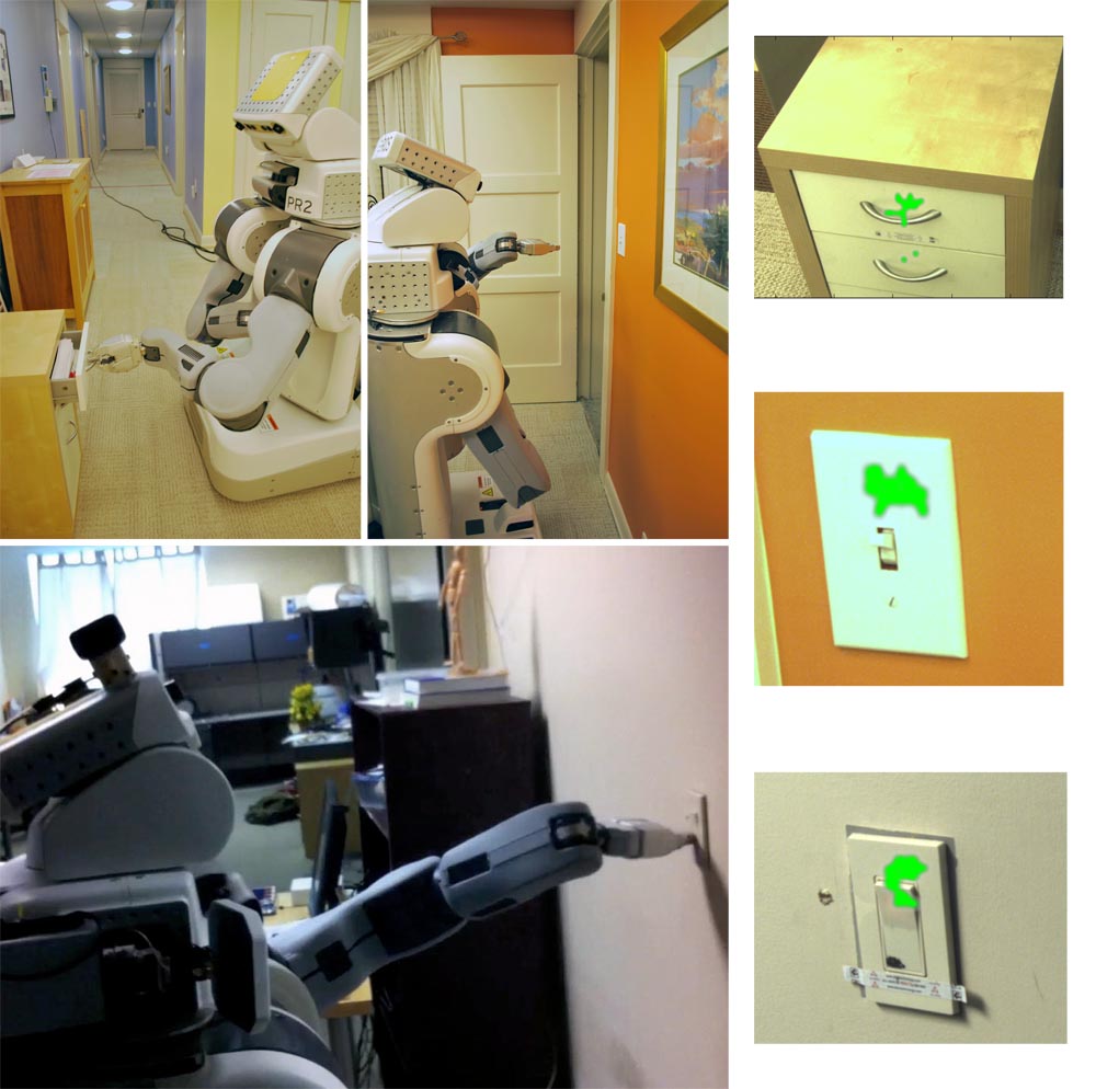
Informing robot manipulation with computer vision continues to be a challenging problem in unstructured human environments, such as homes. Two types of challenges are particularly notable. First, the robot must handle wide variation in the appearance of task-relevant components of the world that can affect its ability to perform tasks successfully. Lighting can vary from home to home and from hour to hour due to indoor lighting and windows. In addition, important components, such as drawer handles and the drawer faces that serve as background, can be distinctive or even unique. The perspective from which a mobile robot observes the component will also vary.
Second, the relationship between the appearance of task-relevant components and the success or failure of a manipulation behavior is complex. For example, the mechanics of a specific device may require that the robot act at a distinct location, such as a finicky drawer that needs to be pushed in the center to be closed, or a convoluted handle that the robot’s gripper can only grasp at particular locations. The robot itself may also change over time and thus alter the relationship between visual appearance and a manipulation behavior, as parts of its body settle, deform, and wear.
One potential solution to these two problems is for robots to autonomously learn how specific objects respond to manipulation attempts using a behavior, and to continue to learn as they perform tasks. By using self-generated data, robots can learn direct mappings from visual features to the input parameters for behaviors, enabling robust execution despite errors in calibration, variations in robot pose, sensor noise, unexpected environmental interactions, and other factors. By continuing to learn over time, robots can also adapt to changes in the environment, the objects, and their bodies.
In this work, we present a system that enables mobile manipulators to autonomously gather data about the execution of behaviors to improve their likelihood of success in future attempts. Our work advances autonomous robot learning in three ways. First, our research addresses challenges of learning in scenarios that integrate mobility and manipulation. During our tests, the robot navigates to the device from various places in the environment. Our approach uses a robot’s mobility as an integral part of autonomous learning, which enables the robot to handle the significant task variation introduced by its mobility. Second, we show that autonomously learning to visually predict where a behavior will be successful can be tractable in real-world scenarios. By using active learning, the robots in our tests learned each visual function after fewer than 150 interactions with each device, even though the robot started from scratch and only used data it collected. The learned visual functions enabled the robots to successfully operate the devices and also have intuitive interpretations. Third, our methods autonomously learn to operate devices that have an approximately binary state, such as a light switch being up or down or a drawer being open or closed. This presents a challenge, since the robot’s actions change the state of the world, which deters the robot from trying the same action again. For example, it would be difficult to learn to open a drawer if, once it is open, the robot is unable to close it. Our system addresses this difficulty by simultaneously training pairs of behaviors and alternating between them as necessary. We also formalize the ideal relationship between these pairs of behaviors and name them complementary behaviors.
We evaluated our system using an implementation on a Willow Garage PR2 robot willow_website at the Aware Home, which is a free-standing house at the Georgia Institute of Technology constructed to test new technologies. First, the robot autonomously learned to operate 6 devices. After learning, we tested the robot’s performance in trials with each of the 6 devices for a total of 110 trials (110 trials (5 devices 2 behaviors 10 trials) (1 device 2 behaviors 5 trials)). In all 110 trials, the robot autonomously operated the device successfully after at most two attempts. If the first attempt failed, the robot autonomously detected the failure and then retrained using this new negative example prior to autonomously trying a second time. We tested opening and closing drawers, turning on and off light switches, and turning on and off rocker switches. Figure 1 shows example output from the resulting trained classifiers, which classify image feature vectors as being associated with success or failure of a behavior.
2 Related Work
There is a significant body of work on robots learning to manipulate autonomously, robots learning to perceive, perception for manipulation that exploits task structure, and active learning methods for using labeling efforts efficiently. In this section, we discuss the relationship between our work and current learning methods as well as work that has demonstrated the effectiveness of using task-relevant cues for perception in human environments. The research we present in this paper builds on our earlier workshop publication nguyen2011 .
2.1 Robot Learning
Even though the use of learning-based methods can yield powerful detectors, labeled training examples are often time consuming and expensive to obtain. Different robot learning methods such as imitation learning, interactive learning and developmental learning lungarella2003a ; pfeifer1997 can be grouped by how they approach the issue of gathering data. We now discuss different forms of robot learning methods and specifically work that involves autonomous learning, where the robot learns with little or no human input after an initialization or teaching period.
2.1.1 Autonomously Learning to Act
Developmental learning research primarily uses data from the robot’s own interactions with its environment and emphasizes scenarios inspired by the development of biological organisms lungarella2003 . Examples include studies of gaze control berthouze1997 ; berthouze1998 ; butko2010 , reaching metta1999 ; hulse2011 , pointing marjanovic1996 , and poking metta2003 .
In the manipulation literature there has also been interest in using autonomous learning based methods to find stable grasps. One of the earliest investigations in grasp learning is by Dunn and Segen dunn88 ) that matched objects using visual features and learned candidate grasps through trial and error. In Zhang2004 , instead of learning one grasping classifier the system learned separate classifiers for grasp position and grasp orientation. Saxena et al. Saxena2008 presented a method that learned a grasp point classifier using a data set of simulated grasps and was able to show success in grasping real objects in uncluttered environments. Similarly, researchers in Erkan2010 also showed a grasp learning algorithm, mapping from 3D edge features using an active learning approach combined with semi-supervised learning. The authors of Klingbeil2008 used a supervised classifier to detect handles and distinguish between left and right facing versions. Work in Montesano2009 from the developmental learning community views the same problem as one of learning object affordances and proposed a method for estimating grasp densities in images of objects on plain backgrounds.
Research on learning from demonstration has investigated how to learn policies and controllers for manipulation but, in most cases, has not addressed perceptual challenges. We refer readers to Argall08 for an extensive survey of existing methods.
While many projects focus on inferring policies from human demonstrations Argall08 , there is a subset of work where autonomous learning is used with dynamic motion primitives ijspeert03 to refine initial human demonstrations. Using this framework, Kober2010 present methods for parameterizing motions refined from human demonstrations based on task objectives. More recently, Pastor et al. Pastor2011 implemented this framework on the PR2 robot to show the PR2 flipping a box using chopsticks and playing pool. In contrast, work in the domain of helicopter acrobatic flights tang10 used a combination of human demonstrations and approximate models, instead of real world practice, to extract intended trajectories from sets of noisy demonstrations. In the system presented by by Prats et al. prats12 , the authors eschewed trajectories and instead focused on creating a system that records task properties in terms of forces applied with respect to a user-defined visual reference frame.
Using a generative method with a planning framework, Stulp et al. stulp12 introduced the concept of action-related places, modeling how a robot’s navigational uncertainty affects its ability to execute grasps.
2.1.2 Autonomously Learning to Perceive
In contrast to motor learning, most work in learning for perception relies on data captured manually ponce2006 , captured in simulation Klingbeil2008 ; Saxena2008 , or downloaded from the web semantic_robot ; chatzilari2011 . Although large data sets can be collected from these sources, the data generated can be biased and may not match what the robot will encounter. Likewise, the relationship between these data and the robot’s actions may not be clear. For example, a good location for a person to grasp or a location that a person believes would be good for grasping may not be appropriate for a robot, given its end effector and other differences. Additionally, there are challenges in processing and generating such data. Text on the web is written in natural language for human beings tenorth11 . Well-framed aesthetically pleasing images can be misleading for robots using noisy sensors from opportunistic points of view. Accurate simulation of physical objects can also be hard to obtain abbeel06b .
The system that we present uses data generated from self-experience, (similar to salganicoff1996 ; Erkan2010 ; Pastor2011 , and Kober2010 ). With self-generated data, generalization becomes less of an issue as the training data and data encountered online are sampled from the same distribution. Even so, labeled examples can be costly to obtain. Interactions with the environment take time, and can potentially result in damage to the environment and the robot. Human labeling can be labor intensive and have errors, ambiguity, and inconsistencies barriuso12 . We address this issue in our work by combining active learning, which reduces the number of examples needed, with autonomous learning methods that eliminate the need for human labeling beyond an initialization process.
Past work in learning for perceptual categorization, a process where agents learn through interaction with the world to divide sensory information into distinct groupings, has used robot self-generated data. However, most systems were designed to classify only simple geometric objects such as cylinders and rectangles using cross-modal information krichmar2002 ; coelho2001 ; scheier1996 .
A relatively small subset of work investigates more complex objects found in human environments. In stober2011 , Stober et al. demonstrated an approach for extracting spatial and geometric information from raw sensorimotor data. Sukhoy and Stoytchev Sukhoy2010 presented an active learning method for a robot pressing doorbell buttons. Kraft et al. kraft2010 presented a system that gradually learns object representations and associates them with object-specific grasps. Katz and Brock in Katz2008a showed a method with which a robot determines the structure of articulated objects through experimentation. Similarly, Hoof et al. hoof12 presented a system that selects maximally informative actions to segment tabletop scenes.
Paolini et al. in paolini12 present related work in which a stationary robot estimates which parameters to provide to a robot behavior based on experience. Like our approach, the parameters to the behavior are in terms of a location. For them, the parameters to the behavior describe the pose of a highlighter held in the robot’s gripper and the behavior attempts to stand the highlighter upright. Their approach uses estimated probability distributions, including a distribution that gives the probability of the marker’s pose conditioned on haptic sensing. In contrast, we use a discriminative approach and directly map visual sensing to 3D locations that are likely to result in success of the behavior.
The work of Sukhoy2010 is notable for its similarity to our approach. They presented a system that uses an uncertainty sampling scheme to actively learn the appearance of doorbell buttons. In contrast, our approach uses a different active learning algorithm, works with a mobile manipulator operating in situ devices, and handles persistent change to the state of the world.
2.2 Task-Relevant Feature Detection
In a parallel thread to robot learning, there has been recognition in the mobile manipulation community of the importance of exploiting task structure to reduce the complexity of operating in the real-world. This point was argued by Katz et al. in Katz2008 . Dang and Allen Dang2010 showed evidence that many manipulation tasks can be described using sequences of rotations and translations. Additionally, work in articulated object perception Katz2008a , tool tip detection Kemp2006 , door handle detection Klingbeil2008 , behavior-based grasping Jain2009 , and corner detection for towel folding Maitin-shepard2010 suggests that, in many tasks, recovery of complex representations of the state of objects prior to manipulation is unnecessary. For example, Jain and Kemp advait10 demonstrated that overhead grasping of diverse real-world objects can be successfully accomplished by representing a segmented object as a planar ellipse. In addition to detecting features used to parameterize manipulation behaviors, task specific cues can be employed to verify the effects of a robot’s actions. For example, Okada et al. have demonstrated the value of task-specific perception for success detection by humanoid robots, including detecting that liquid is flowing okada06 . These systems illustrate that low-dimensional task-specific object representations can result in good performance over real-world variation. However, they used hand-coded and hand-trained feature detectors that required significant engineering effort. With our approach, robots autonomously learn to classify visual features as being relevant to the success of a specific behavior or not.
2.3 Active Learning and Curiosity Driven Learning
In many robot learning scenarios, unlabeled data can be readily acquired but labeling the data is costly. Researchers have proposed the use of active learning methods settles12 to gain more value from limited labeling. In many active learning algorithms, at each iterative learning step the learner is given an option to select a data point to be labeled out of a set of unlabeled data points. For one class of proposed approaches, the learner picks the data point whose label it is most uncertain about lewis94 ; culotta05 ; settles08 . With disagreement-based methods, learner ensembles select the data point they most disagree on cohn94 . More computationally demanding methods, however, attempt to explicitly minimize future expected error or variance roy01 ; berger96 ; lafferty01 . There are also proposals to combine semi-supervised and active learning to exploit structure in unlabeled data mccallum98 ; muslea02 ; zhu03 . Although there have been several large scale studies of active learning methods on different data sets showing its superiority over randomly picking data points for labeling korner06 ; schein07 ; settles08 , the best active learning algorithm to use in each circumstance is application specific. In our work, we use a heuristic that picks the data point closest to the decision boundary of a support vector machine (SVM) for labeling, a method that has been shown to perform well in a variety of applications jain10b ; Schohn2000 ; tong00 .
3 Approach
Our approach enables a mobile manipulator to autonomously learn a function that takes a 2D RGB image and a registered 3D point cloud as input and returns a 3D location at which a manipulation behavior is likely to succeed. Our approach requires a pair of manipulation behaviors, verification functions that detect when each behavior has been successful, and an initial hint as to where one of the behaviors will be successful.
Each behavior must have input parameters that correspond with a 3D location that specifies where the behavior will act. During training, our system executes each behavior multiple times using different 3D locations around the device being manipulated and records whether or not the behavior succeeded at each location. For each 3D location, the system creates an image feature vector using an area of the registered 2D RGB image associated with the 3D location. These image feature vectors are labeled with whether or not the behavior succeeded or failed at their associated 3D locations. In other words, the collected data set consists of positive and negative examples of image feature vectors that were or were not associated with the success of the behavior. With a classifier trained from this data set, the robot can then predict if the associated behavior will succeed at a 3D location based on the image feature vector associated with the location.
To avoid user intervention during training, our procedure trains two behaviors at the same time, switching to the other behavior when the current behavior succeeds. This enables our method to operate devices that can be approximated as having two binary states, such as a drawer being open or closed. Using a pair of behaviors allows the robot to change the device back and forth between these two states, so that training can continue autonomously. For example, instead of training a drawer opening behavior in isolation, our process flips to training a drawer closing behavior when opening succeeds and vice versa until the classifier converges. We also formalize the relationship between the two behaviors and define them as complementary behaviors.
Using self-generated data takes considerable time, since each labeled image feature vector requires that the robot execute the behavior at a 3D location and observe the results. To avoid needing an intractable number of trials, our method uses active learning to execute the behavior at an informative 3D location at each iteration. Specifically, our procedure trains a support vector machine (SVM) after each trial using the current labeled data. It then uses a heuristic proposed by Shohn and Cohn Schohn2000 to select the unlabeled image feature vector that is closest to the current SVM’s decision boundary to be labeled next. It then executes the behavior at the 3D location associated with this image feature vector.
Our training procedure has two phases. The first is an initialization phase where the user selects the behavior pair to train, gives a seed 3D location, and positions the robot’s mobile base for training. The next phase is an autonomous phase where the SVM active learning procedure runs until the learner converges. After convergence, each behavior has a classifier that predicts 3D locations where it will succeed.
During runtime, if the behavior’s verification function detects a failed attempt, our procedure appends this negative example to the data set, retrains the classifier, and tries again using the output of this new classifier (Section 3.3.3).
In the following sections, we discuss the requirements of our learning procedure 3.1, properties of complementary behaviors (Section 3.2), our training procedure in detail (Section 3.3), and classification infrastructure (Section 3.4).
3.1 Requirements
For our algorithm to apply, several assumptions must be met. First, our approach assumes that the robot can execute a set of behaviors, each of which only requires a 3D location in the robot’s frame of reference as initial input. We have demonstrated that this is a reasonable assumption for a variety of useful mobile manipulation behaviors in our previous work on laser pointer interfaces nguyen08 .
Second, this approach assumes that the robot has a way of reliably detecting whether or not a behavior it has executed was successful or not. Our approach assumes that the verification function, , returns whether or not a behavior succeeded. For this work, it takes the form , where is the array of robot sensor readings when the state of the world is . The states and are the states before and after the robot executes a behavior.
Third, the approach assumes that for each behavior, , there is a complementary behavior, . If successfully executes, then successful execution of will return the world to a state that allows to execute again. We discuss the implications of this requirement in Section 3.2.
Fourth, each behavior must return a 3D location indicating an approximate location where its complementary behavior should execute. This requirement is provided as a device for the behavior pair to communicate the position of the object manipulated to each other. These requirements can be summarized as:
| (1) | |||
| (2) |
3.2 Complementary Behaviors
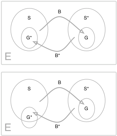
In order to train autonomously, without human intervention, our procedure uses a complementary pair of behaviors during its data gathering process. We introduce the notion of a complementary robot behavior to a behavior as being a behavior that is capable of “reversing” the state of the world, so that behavior can be used again. For example, if behavior ’s function is to turn off the lights using a light switch, its complement, , would turn the lights back on using that light switch. If a behavior opens a door, then its complement would close the door.
We formalize our notion of complementary behaviors by defining the relationship between ideal complementary behaviors. We first define a hypothetical state space that contains the states of everything in the world, including the robot’s state. We then represent execution of behavior given an initial state of the world as , where is an operator that takes the initial state of the world as input and returns the resulting state of the world . Furthermore, when is applied to a state , where is a set of starting states, it returns , where is a set of goal states. We define
| (3) |
and
| (4) |
Intuitively, if the state of the world, , is a start state, , then the behavior will be successful and the resulting state of the world, , will be a goal state, .
We now define a complement of behavior to have a set of start states, , and a set of goal states, , such that and (see Figure 2). This guarantees that applying ’s complement, , after successfully applying will result in a state of the world that allows to once again be applied successfully. More formally, it guarantees that when , and that when .
3.3 Autonomous Training
3.3.1 Initialization
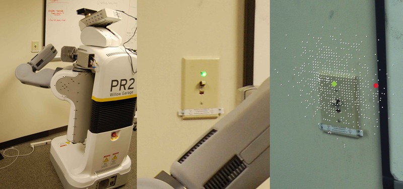
Our initialization procedure is motivated by the scenario in which a user would take the robot on a home tour and point out 3D locations using a green laser pointer nguyen08 and specify behaviors applicable to those locations. After this tour, the robot would later autonomously navigate back and learn to robustly perform the behaviors.
For this paper, we have implemented an initialization procedure that starts with the user navigating the robot to be in front of the device to be operated using a gamepad interface. Then using a green laser pointer nguyen08 , the user designates an initial 3D location to begin exploring. The robot samples 3D points around this designated location (using a spherical Gaussian with a variance of 4 cm) and executes the behavior pair with respect to them. After each execution of a behavior at a 3D location, the behavior’s verification function returns a label of either success or failure. The sampling process continues until the procedure gathers data points from at least one successful and one failed trial. These two data points are then used to train SVM classifiers that guide the data gathering process with the active learning heuristic Schohn2000 .
After this initialization, the robot stores a 2D mobile base pose with respect to a global map, the user provided 3D location, an SVM trained using two labeled data points, and labels indicating which pair of behaviors is applicable at the specified location. We illustrate this procedure in Figure 4. In addition, the user navigates the robot to eight different poses in the room, referred to as practice poses, each at least a half meter away from the device. The robot also stores the 2D mobile base poses associated with these eight practice poses.
3.3.2 Training Procedure
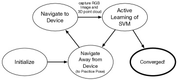
Our training procedure is designed to emulate conditions that the robot would encounter when performing the task. After receiving a command, the robot navigates to the device so that it can execute the commanded behavior. Navigation and localization errors result in variations that can substantially reduce the performance of a behavior, such as variation in the robot’s point of view. We illustrate task variation due to navigation in Figure 6. Our training method samples from this source of task variation by commanding the robot to navigate to one of eight practice poses in the room and then commanding it to navigate back to the device (see Figure 5).
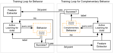
After navigating to the device, our procedure begins an active learning phase (see Figure 3). We summarize this phase in Algorithm 1. The process starts with the robot capturing an RGB image and a registered 3D point cloud. The robot then computes image feature vectors for 3D points randomly sampled from the point cloud around the device (extract_features). It then iteratively selects image feature vectors (svm_pick) that it labels by executing the behavior at the associated 3D location and using the verification function (execute_behavior). After each trial, the process retrains the SVM classifier with a data set that incorporates the newly acquired example (add_instance_and_retrain_svm). The procedure stops after gathering a maximum of six labeled image feature vectors or the learner converges (stop_criteria). We imposed this conservative maximum limit because image feature vectors gathered from the same view are correlated, which can confuse the learning heuristic and result in the training process stopping prematurely. If the robot operates the device successfully in a trial, the algorithm continues, but uses the complementary behavior for the next iteration (section following If(success)).
This process continues until svm_converge is satisfied for each of the eight practice poses. Once it is satisfied for a particular practice pose, the robot no longer navigates to the pose. We define convergence for a practice pose to occur when after driving up to the device from the practice pose, none of the initially computed image feature vectors are closer to the decision boundary than the current support vectors.
3.3.3 Behavior Execution Procedure
The training process above produces a classifier that can reliably detect locations where the associated behavior will succeed. To use this classifier, our robot navigates to the device using the 2D map pose stored during initialization, classifies 3D points in the view that it sees, finds the mode of the positive classified points using kernel density estimation scipy_kde , selects the 3D point in the point cloud closest to this mode, and executes the associated behavior using the resulting 3D location.
If the behavior fails to execute using this 3D location, our procedure adds the associated image feature vector as a negative example to the data set and retrains the classifier. This new example changes the classifier’s decision boundary. The robot then selects a new 3D location using the retrained classifier with the originally computed image feature vectors. This continues until the behavior is successful. It then adds the image feature vector associated with this success to the data set as a positive example and retrains the SVM. In contrast to systems where the execution process is independent of data gathering and training, the robot has the opportunity to retrain its classifier when it detects errors made during execution, giving the possibility of lifelong training.
3.4 Classification
The base classifier that we use in this work is a support vector machine (SVM). As is standard in supervised classification, given a data set of labeled examples with representing feature vector i of local 2D appearance information associated with a candidate 3D point and where positive and negative denote, respectively, success and failure, we want to be able to predict for a future instance .
As functional structures on many household devices are often small compared to nonfunctional components, such as the size of a switch relative to the plate or wall, there is typically an unbalanced data set problem, since there can be many more negative than positive examples. In unbalanced data sets the SVM can return trivial solutions that misclassify all the positive samples, since the misclassification cost term in the SVM objective is defined over all samples. To prevent this issue, we use an SVM formulation that separates the costs of misclassifying the negative class from the cost of misclassifying the positive class Chang2011 ,
| (5) | |||||
where and b are SVM parameters, counts the margin violations for misclassified points (in the case of nonseparable data), and is the radial basis kernel function we use (discussed in Section 4.1).
This formulation separates the SVM misclassification cost scalar into and which are, respectively, costs due to negative and positive misclassifications. For our system, we set to be 1, and to be the number of negative examples over the number of positive examples. This scaling keeps the percentage of misclassified positive and negative examples similar in our skewed data set, where there might be many more negative than positive examples. Without this adjustment, we found that training often returned trivial classifiers that classified any input vector as negative.
3.4.1 Active Learning Heuristic
Our training process iteratively builds a data set that it uses to train the classifier. Before each trial, the system selects the image feature vector to label. To select the feature vector, the system uses a heuristic developed in Schohn2000 that selects the feature vector closest to the decision boundary of the existing SVM, under the condition that it is closer to the boundary than the SVM’s support vectors. The procedure converges when no feature vectors remain that are closer to the decision boundary than the support vectors.
At each iteration of our procedure, we define the previous iteration’s data set as , the current set of support vectors as , the unlabeled image feature vectors as , and the SVM distance function, which measures distance to the decision boundary, as . The system selects the unlabeled image feature vector that is closest to the decision boundary as specified by the following expression:
| (6) |
3.4.2 Features
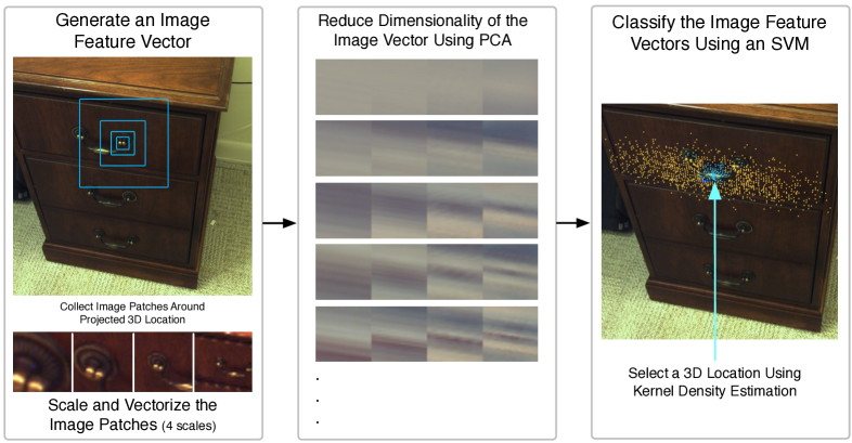
The feature generation procedure, which is illustrated in Figure 7, takes as input a 3D point cloud, a registered high resolution RGB image, and a reference 3D point. The system first selects random 3D points from the point cloud, without replacement, around the reference 3D point according to a Gaussian distribution , where with and being, respectively, variances in the x, y, and z direction. The Gaussian mean is set to the 3D reference point. This Gaussian search prior enables the system to save computational effort and focus its attention on the device that the robot is supposed to manipulate.
After randomly selecting a set of 3D points, the system projects each 3D point into the high resolution RGB image, . For each projected 3D point, it collects square image patches of successively increasing size centered at the projected 2D point in the RGB image, scales these patches to have the same height and width, vectorizes them, and concatenates them into an image feature vector. The system then uses Principle Components Analysis (PCA) to reduce the dimensionality of these image feature vectors. We discuss the specifics of these steps in Section 4.1.
4 Implementation
4.1 Learner Parameters
We implemented our system on on a PR2 robot willow_website : a mobile manipulator produced by Willow Garage with two arms, an omnidirectional base, and a large suite of sensors. Our system uses 3D point clouds and 5 megapixel RGB images from the robot’s tilting laser range finder and Prosilica camera.
Starting with a 3D point cloud and registered RGB image, our process randomly selects 3D points from the point cloud as described in Section 3.4.2. For each selected 3D point, the system collects image patches at 4 scales centered around the point’s 2D projection in the RGB image. The raw image patches have widths of 41, 81, 161, and 321 pixels. They are then scaled down to be 31x31 pixel image patches, vectorized, and concatenated into an 11,532 element image feature vector for each 3D point. The vectors are then reduced to 50 element vectors by projecting them onto PCA basis vectors that are calculated for each action using the 11,532 element image feature vectors computed from the first 3D point cloud and RGB image captured during initialization.
To classify these 50 dimensional image feature vectors, we use SVMs with radial basis function kernels. We set the hyperparameters of this kernel using an artificially labeled data set. To create the data set we took 10 different 3D point clouds and RGB images of a light switch from different views and geometrically registered them. After hand-labeling one 3D point cloud and RGB image, we geometrically propagated labels to the other 9. To find the kernel hyperparameters, we split the labeled image feature vectors from this data set into a training set and a test set. We then performed a grid search Chang2011 for the set of hyperparameters that best generalized to unseen data in the test set.
4.2 Behaviors
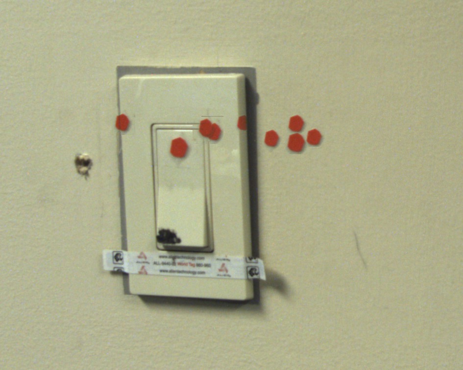
To evaluate our system, we implemented three pairs of complementary behaviors that operate light switches, rocker switches and drawers. These tasks are sensitive to the location at which an action is performed. For example, light switches are small targets that require high precision and accuracy for the PR2 to operate with its finger tips. As illustrated in Figure 6, we have found that a PR2 will rarely succeed at flipping a light switch if it simply navigates to a pre-recorded location and moves the arm through a pre-recorded motion without visual feedback.
4.3 Light Switch Behaviors
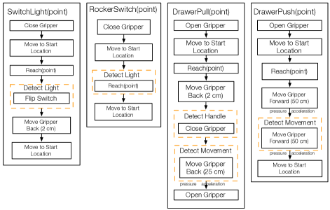
Our light switch behavior’s strategy is to reach forward to the specified 3D location, stop on contact detected with gripper tip tactile sensors, then slide along the contacted surface in the direction of the switch. A successful 3D location needs to place the robot’s finger so that its width will make contact with the switch and far enough above or below the switch so that the finger will move the switch down or up. Figure 8 shows the sequence of actions taken by this behavior.
The behavior starts with the robot closing its gripper (Close Gripper), moving the gripper to a pre/manipulation location (Move to Start Location), reaching to the given 3D location (Reach), flipping the switch by sliding along the flat surface (Flip Switch), moving the gripper back (Move Gripper Back), then moving back to the initial location (Move to Start Location).
There are a few steps in this behavior where the robot detects tactile events. When reaching, the robot stops when it detects contact using pressure sensors on its finger tips. Next, the sliding movement stops after detecting a spike in acceleration with the accelerometer embedded in the robot’s gripper. In the context of this task, this spike in acceleration typically corresponds with the light switch flipping.
To detect success, our behavior measures the difference between the average intensity of an image captured before sliding along the surface and an image captured after. A large difference indicates that the lighting intensity changed.
The complementary behavior is identical except for a change in the direction of flipping. After executing, the behavior and complementary behavior return the 3D location input with a predefined offset ( 8 cm).
4.4 Rocker Switch Behaviors
Our rocker switch behavior consists solely of a reaching out step similar to the light switch behavior above, since the force applied from contact during the reach procedure is enough to activate the switch. A successful 3D location will result in the robot’s fingers pushing in the top or bottom of the rocker switch.
This behavior uses the same image differencing method to detect success as the light switch behavior. It calculates the difference between images captured before and after the robot reaches forward. After executing, the behavior and complementary behavior return the 3D location with a predefined offset ( 5 cm).
4.5 Drawer Behaviors
Pulling open and pushing closed a drawer require different behaviors and success detection methods. Our pulling behavior reaches to the drawer handle location, detects contact, moves back slightly, grasps with the reactive grasper from hsiao2010 , and pulls. When pulling, failure is detected if the grasp fails or the robot fails to pull for at least 10 cm while in contact with the handle. A successful 3D location will result in the robot’s gripper grasping the handle well enough to pull it back by at least 10 cm. When pushing, failure is detected if the gripper does not remain in contact with the surface for at least 10 cm. This classifies events where the robot pushes against a closed drawer or an immovable part of the environment as failures. After executing, the behavior and complementary behavior return the 3D location the tip of the gripper was in immediately after pulling or pushing.
5 Evaluation
We evaluated our system using six separate devices. We first tested on a rocker switch using the PR2 robot named GATSBII in our lab, the Healthcare Robotics Lab (HRL). For the remaining five devices we performed tests in the Georgia Tech Aware Home, a residential lab on campus used as a test bed for new technologies.
In each environment, we began our evaluation by creating an occupancy grid map of the area with the PR2’s built-in navigation package eitan2010 . Then, after initialization (Section 3.3.1), we ran the autonomous training system (Section 3.3.2) until convergence. The experimenter provided 8 practice poses in the room representative of places from which the robot might travel. The autonomous training system ran without experimenter intervention except for pausing and resuming when the robot’s batteries ran low. In all, we trained 12 classifiers, a result of having 6 devices and a pair of behaviors for each device (12 6 2).
After finishing the training sessions, we evaluated each classifier by running each behavior multiple times, giving 110 trials in all (110 trials (5 devices 2 behaviors 10 trials) (1 device 2 behaviors 5 trials)). During each trial we allowed the behavior to retry and incorporate information from failures if it did not succeed the first time. However, we discarded any data gathered during the retry procedure by previous trials at the start of each new trial to obtain accurate error statistics for the original classifier.
For the devices we used in our evaluation, the functional components are difficult for the PR2’s laser range finder to detect. Light switches only show up as a few protruding 3D points similar to other noisy 3D points produced by the sensor. The rocker switch appears as a flat 2D texture on the 3D point cloud. Drawer handles tend to be metallic and reflective resulting in an absence of 3D points. Using features from RGB images enabled the robot to overcome these challenges.
5.0.1 Effects of Navigation Errors
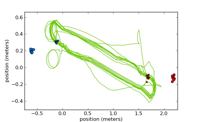
To better understand the variation in the task due to the robot’s mobility, we investigated how the pose of the PR2 varies when navigating to a goal pose. Using a room equipped with a NaturalPoint OptiTrak motion capture system, we tracked the pose of the PR2 and commanded the robot to navigate back and forth to two goal poses 10 times each. As the standard deviation of the robot’s Cartesian position does not represent angular errors, we calculated errors for a point 50 cm in front of the robot, which is representative of where a device would be located. The standard deviation of the location in front of the robot was 1.85 cm, and 1.79 cm in the x and y directions, respectively. For the second position, the standard deviation was 1.55 cm and 2.38 cm in the x and y directions, respectively. We show the results of this experiment in Figure 9. These errors demonstrate that navigating to a pre-recorded location and moving the arm through a pre-recorded motion would result in large variation that can result in failure. For example, the robot’s finger tips are 2.0 cm wide and light switches are only 0.8 cm wide.
5.1 Results
| Action | Positive Ex. | Negative Ex. | Total |
|---|---|---|---|
| HRL Rocker On | 49 | 96 | 145 |
| HRL Rocker Off | 47 | 94 | 141 |
| Aware H. Rocker On | 26 | 47 | 73 |
| Aware H. Rocker Off | 29 | 52 | 81 |
| Ikea Drawer Open | 23 | 35 | 58 |
| Ikea Drawer Close | 23 | 39 | 62 |
| Brown Drawer Open | 21 | 62 | 83 |
| Brown Drawer Close | 25 | 46 | 71 |
| Orange Switch On | 17 | 43 | 60 |
| Orange Switch Off | 20 | 31 | 51 |
| Ornate Switch On | 38 | 66 | 104 |
| Ornate Switch Off | 40 | 76 | 116 |
| Action | Try | Try |
|---|---|---|
| HSI Rocker On | 2 | 3 |
| HSI Rocker Off | 4 | 1 |
| Aware Home Rocker On | 10 | |
| Aware Home Rocker Off | 9 | 1 |
| Ikea Drawer Open | 10 | |
| Ikea Drawer Close | 10 | |
| Brown Drawer Open | 10 | |
| Brown Drawer Close | 10 | |
| Orange Switch On | 8 | 2 |
| Orange Switch Off | 9 | 1 |
| Ornate Switch On | 9 | 1 |
| Ornate Switch Off | 9 | 1 |
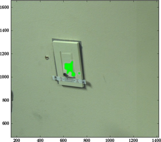
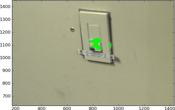
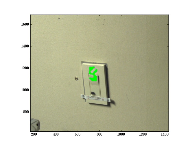
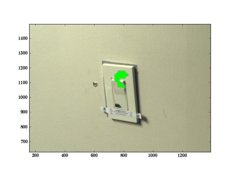
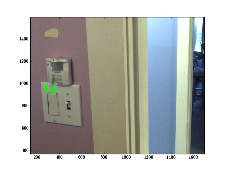
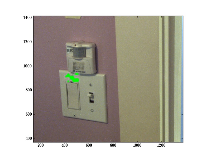
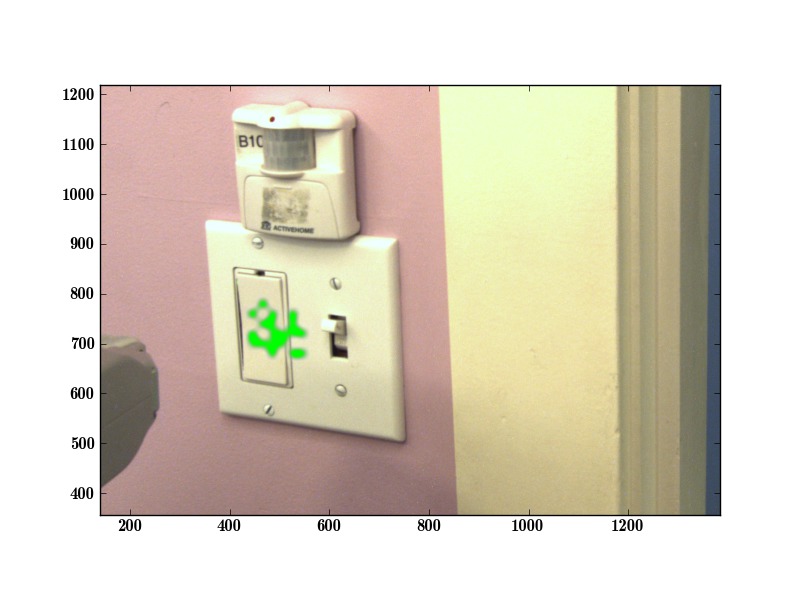
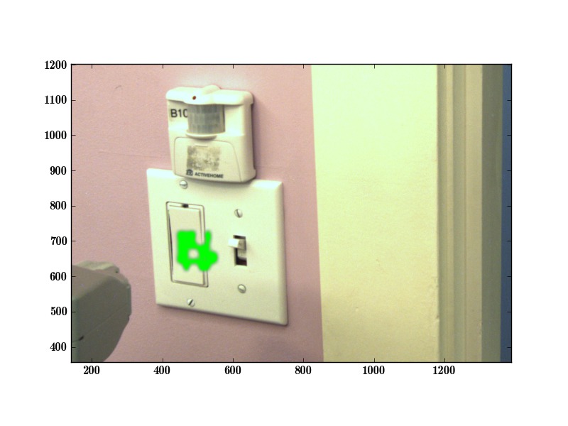
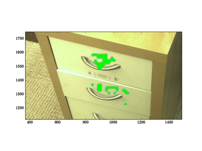
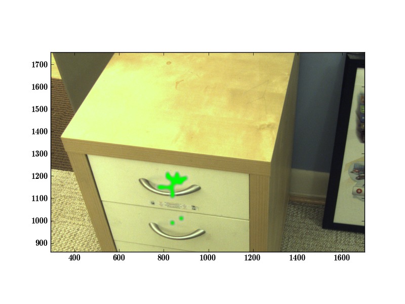
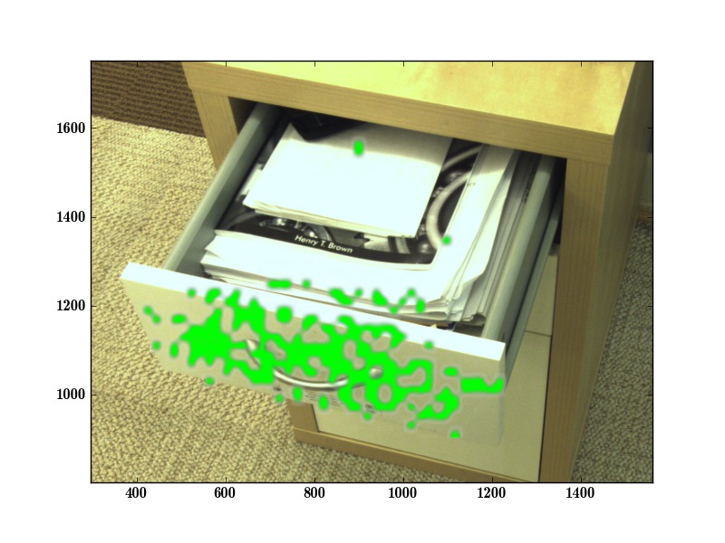
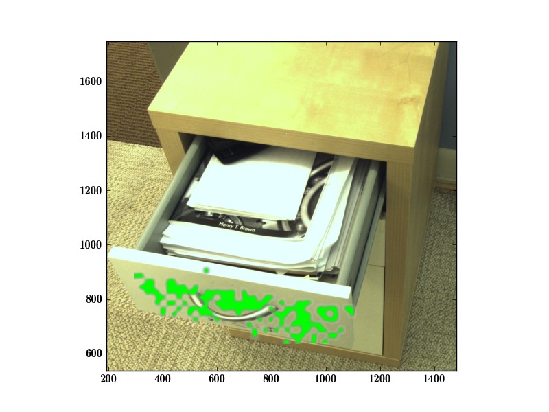
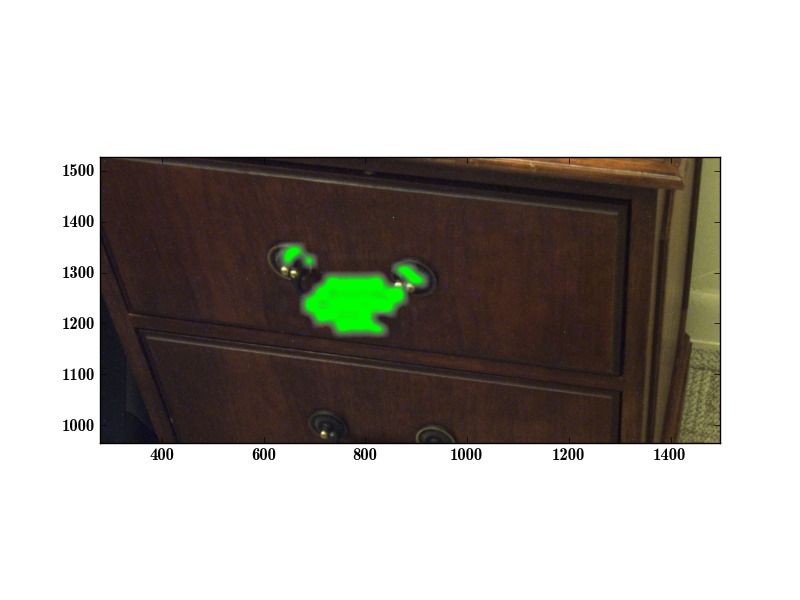
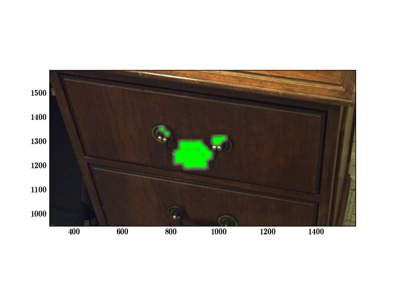
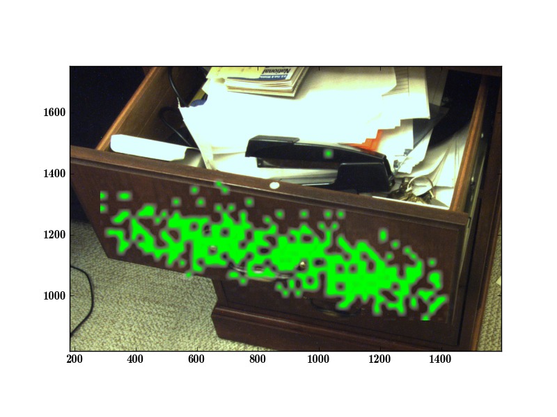
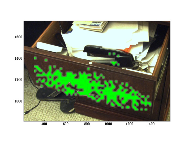
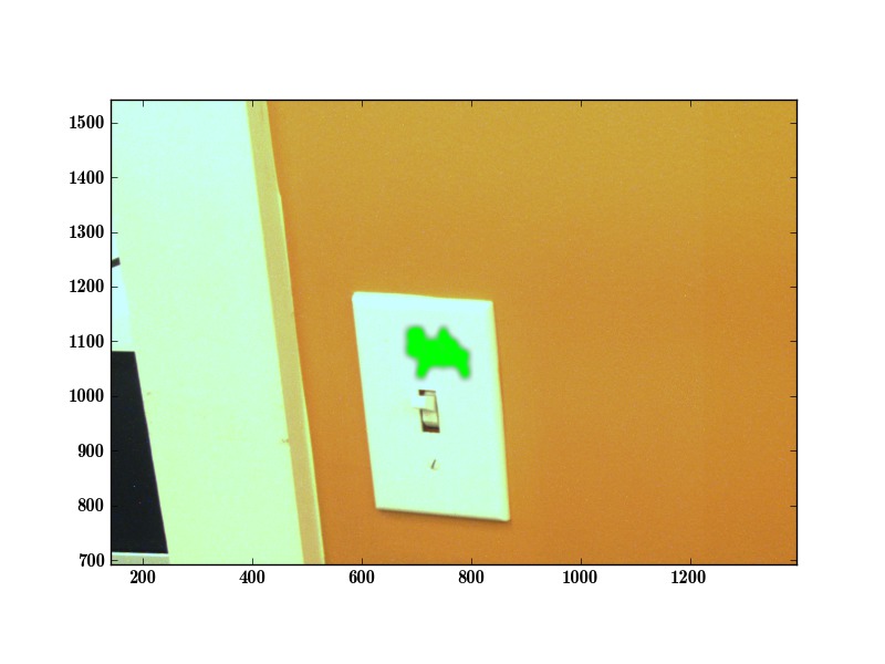
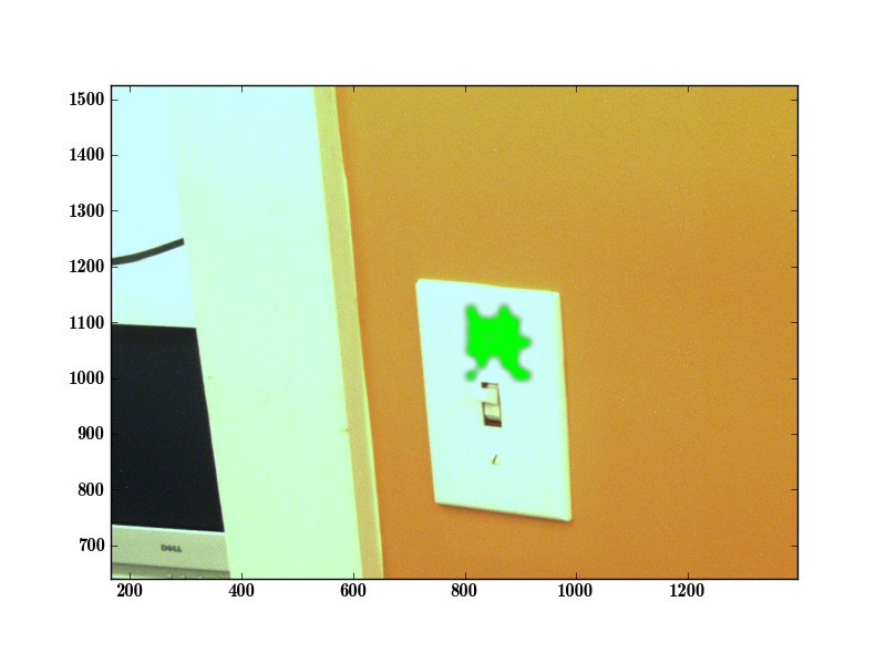
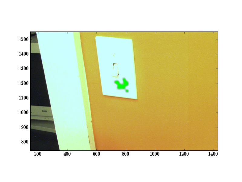
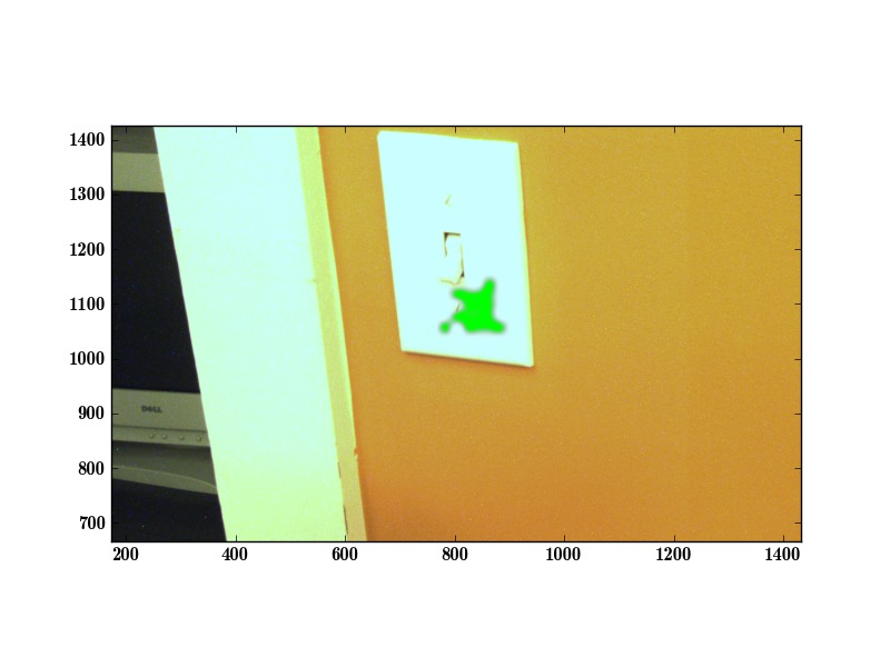
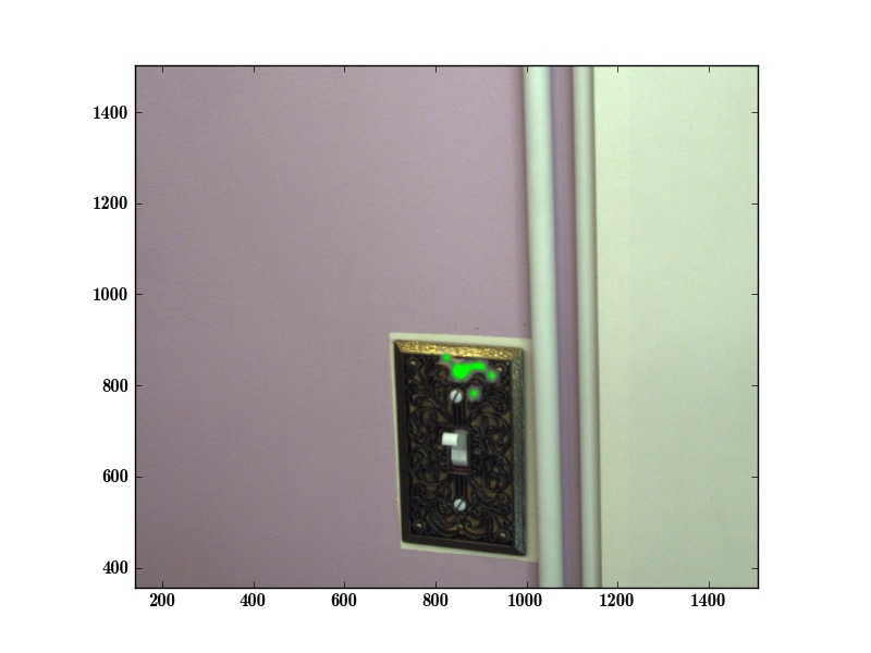
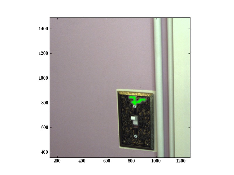
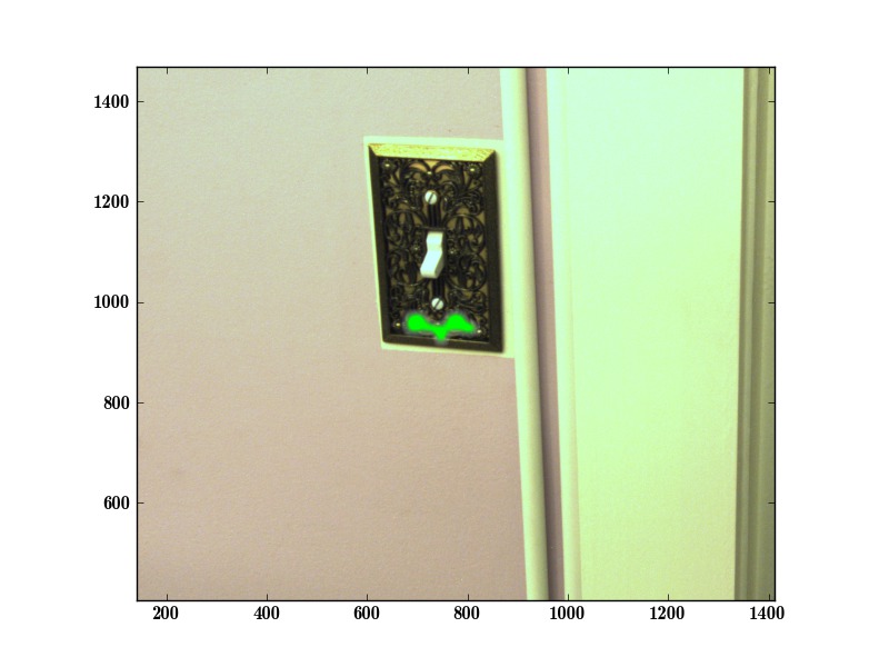
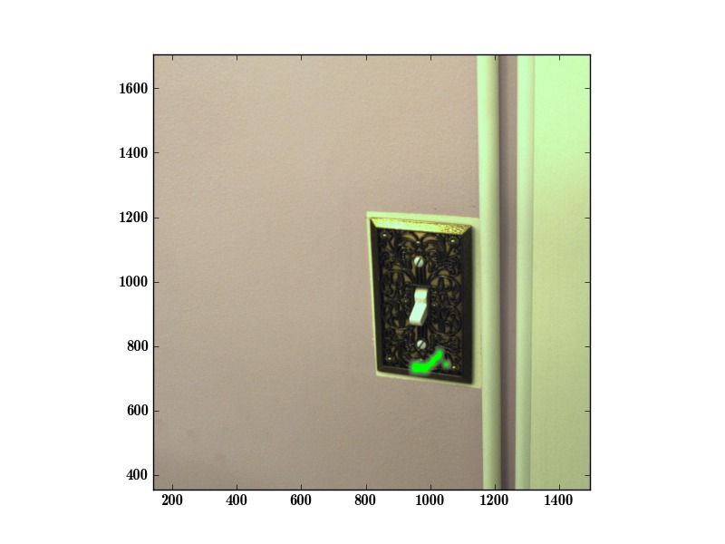
Figure 10 shows the locations that the autonomously trained SVMs predict will be likely to lead to the success of their associated behaviors. These predictions are solely a function of the visual appearance of each location as represented by its image feature vector. These visualizations of the classifier output demonstrate that the classifiers identify locations relevant to their associated behaviors. For example, the robot autonomously discovers that opening a drawer requires grasping at the location of the drawer handle, while closing a drawer can be performed across the front surface of the drawer. The visualizations also show that different drawer handles can have distinct task-relevant properties. For example, the opening behavior works best when grasping the middle of the silver handle, but can succeed by grasping the far ends of the brass handle.
Due to the distribution for random sampling including some points on the lower handles for the white drawers, the SVM estimates that success can be achieved by pulling on the top handle or the bottom handle. The illustrates a limitation with our current approach, since the verification function for pulling a drawer open can not tell the difference between the top or the bottom drawer. It also shows the influence of the distribution used to randomly sample 3D locations. At the same time, it suggests that the visual classifiers may have some ability to generalize to distinct objects.
For the light switches, the behaviors slide along the surface of the switch. The robot autonomously discovered that locations that are along the switch plate above and below the switch are likely to lead to success. Additionally, it does not predict success for locations along the wall, which is appropriate since the robot’s fingers get caught on the switch plate edge if the robot tries to slide along the wall to the switch.
In Table 1, we show the number of examples collected for each classifier. The median number of examples needed was 77, and the maximum needed was 145 examples. With the rocker switch, where examples are noisy due to the middle of the switch being an unreliable spot to push, the number of examples increased to 145 indicating a sensitivity of our approach to label noise.
Table 2 shows the results of using these trained classifiers after training. Encouragingly, over the 110 trials our behavior execution process attained a 100% success rate after at most two tries. In addition, errors that led to retries usually caused the robot to miss an appropriate location on the device by a small distance.
6 Future Work
There are a number of potential extensions to this work, and interesting issues left to consider. Although we have picked a particular active learning framework, other frameworks might perform better. In addition, currently we assume that each new device is completely new to the robot, but many devices of a particular class have visual similarities. Data from other devices might provide a prior and reduce the training required. Similarly, the structure of successful locations might be shared across devices, even if they are visually distinct. For example, the front surfaces of drawers often being pushable, the centers of drawers often being pullable, and the centers of light switch panels often being switchable could be useful information, even if aspects of their appearances change dramatically.
7 Discussion and Conclusions
In general, there are risks for a robot that learns in human environments and an unrestrained learning system can get into situations that are dangerous to itself, to the environment, or to people. We address this issue by limiting the robot to using a few classes of behaviors in parts of the home that users have designated as safe for robot learning. Additionally, the behaviors move the robot’s arm compliantly and use haptic sensing to decide when to stop moving. By learning in situ, a robot’s data gathering activities do not have to stop after its training phase and can potentially continue for as long as the robot remains in service.
Autonomous learning in human environments is a promising area of research that gives robots methods to cope with devices that they have not encountered before and many forms of real-world variation. We have presented methods that enable a mobile manipulator to autonomously learn to visually predict where manipulation attempts will succeed. As we discussed in the introduction, our work advances autonomous robot learning in three ways. First, our approach uses a robot’s mobility as an integral part of autonomous learning, which enables the robot to handle the significant task variation introduced by its mobility. Second, our research demonstrates that by using active learning, a robot can autonomously learn visual classifiers solely from self-generated data in real-world scenarios with a tractable number of examples. Third, our research introduces complementary behaviors to address challenges associated with autonomously learning tasks that change the state of the world.
Acknowledgments
We thank Aaron Bobick, Jim Rehg, and Tucker Hermans for their input. We thank Willow Garage for the use of a PR2 robot, financial support, and other assistance. This work was funded in part by NSF awards CBET-0932592, CNS-0958545, and IIS-1150157.
References
- [1] Scipy gaussian kde function. http://www.scipy.org/doc/api_docs/SciPy.stats.kde.gaussian_kde.html.
- [2] Willow Garage. http://www.willowgarage.com.
- [3] Semantic robot vision challenge. http://www.semantic-robot-vision-challenge.org/, 2007.
- [4] P. Abbeel, M. Quigley, and A. Y. Ng. Using inaccurate models in reinforcement learning. In International Conference on Machine Learning, 2006.
- [5] B. D. Argall, S. Chernova, M. Veloso, and B. Browning. A survey of robot learning from demonstration. In Robotics and Autonomous Systems, 2008.
- [6] A. Barriuso and A. Torralba. Notes on image annotation. In MIT Tech Note, 2012.
- [7] A. Berger, V. D. Pietra, , and S. D. Pietra. A maximum entropy approach to natural language processing. In Computational Linguistics, 1996.
- [8] L. Berthouze, P. Bakker, and Y. Kuniyoshi. Learning of oculo-motor control: a prelude to robotic imitation. In International Conference on Robotics and Intelligent Systems, 1997.
- [9] L. Berthouze and Y. Kuniyoshi. Emergence and categorization of coordinated visual behavior through embodied interaction. In Machine Learning, 1998.
- [10] N. J. Butko and J. R. Movellan. Developmental robotics architecture for active vision and reaching. In International Conference on Development and Learning, 2010.
- [11] N. J. Butko and J. R. Movellan. Learning to look. In International Conference on Development and Learning, 2010.
- [12] C.-C. Chang and C.-J. Lin. Libsvm : a library for support vector machines. http://www.semantic-robot-vision-challenge.org/, 2001.
- [13] E. Chatzilari, S. Nikolopoulos, S. Papadopoulos, and C. Z. Y. Kompatsiaris. Semi-supervised object recognition using flickr images. In International Workshop on Content-Based Multimedia Indexing, 2011.
- [14] D. L. Christian Scheier. Categorization in a real-world agent using haptic exploration and active perception. In International Conference on Simulation of Adaptive Behavior, 1996.
- [15] J. Coelho, J. Piater, and R. Grupen. Developing haptic and visual perceptual categories for reaching and grasping with a humanoid robot. In Robotics and Autonomous Systems, 2001.
- [16] D. Cohn, L. Atlas, and R. Ladner. Improving generalization with active learning. In Machine Learning, 1994.
- [17] A. Culotta and A. McCallum. Reducing labeling effort for stuctured prediction tasks. In Conference on Artificial Intelligence (AAAI), 2005.
- [18] H. Dang and P. K. Allen. Robot Learning of Everyday Object Manipulations via Human Demonstration. IROS, pages 1284–1289, 2010.
- [19] G. Dunn and J. Segen. Automatic discovery of robotic grasp configuration. In International Conference on Robotics and Automation, 1988.
- [20] A. Erkan, O. Kroemer, R. Detry, Y. Altun, J. Piater, and J. Peters. Learning probabilistic discriminative models of grasp affordances under limited supervision. In IROS, pages 1586–1591. IEEE, 2010.
- [21] K. Hsiao, S. Chitta, M. Ciocarlie, and G. Jones. Contact-reactive grasping of objects with partial shape information. In IROS, 2010.
- [22] A. J. Ijspeert, J. Nakanishi, and S. Schaal. Learning attractor landscapes for learning motor primitives. In Advances in Neural Information Processing Systems (NIPS), 2003.
- [23] A. Jain and C. C. Kemp. EL-E: an assistive mobile manipulator that autonomously fetches objects from flat surfaces. Autonomous Robots, 2009.
- [24] A. Jain and C. C. Kemp. El-e: An assistive mobile manipulator that autonomously fetches objects from flat surfaces. In Autonomous Robots, 2010.
- [25] P. Jain, S. Vijayanarasimhan, and K. Grauman. Hashing hyperplane queries to near points with applications to large-scale active learning. In Advances in Neural Information Processing Systems (NIPS), 2010.
- [26] D. Katz and O. Brock. Manipulating Articulated Objects With Interactive Perception. In ICRA, 2008.
- [27] D. Katz, J. Kenney, and O. Brock. How Can Robots Succeed in Unstructured Environments? In RSS, Robot Manipulation Workshop, 2008.
- [28] C. C. Kemp and A. Edsinger. Robot Manipulation of Human Tools : Autonomous Detection and Control of Task Relevant Features. In ICDL, 2006.
- [29] E. Klingbeil, A. Saxena, and A. Y. Ng. Learning to Open New Doors. In RSS Workshop on Robot Manipulation, 2008.
- [30] J. Kober, E. Oztop, and J. Peters. Reinforcement Learning to adjust Robot Movements to New Situations. In RSS, 2010.
- [31] C. Körner and S. Wrobel. Multi-class ensemble-based active learning. In European Conference on Machine Learning (ECML), 2006.
- [32] D. Kraft, R. Detry, N. Pugeault, E. Başeski, F. Guerin, J. Piater, and N. Krüger. Development of object and grasping knowledge by robot exploration. In IEEE Transactions on Autonomous Mental Development, 2010.
- [33] J. L. Krichmar and G. M. Edelman. Machine psychology: autonomous behavior, perceptual categorization and conditioning in a brain-based device. In Cerebral Cortex, 2002.
- [34] J. Lafferty, A. McCallum, , and F. Pereira. Conditional random fields: Probabilistic models for segmenting and labeling sequence data. In International Conference on Machine Learning (ICML), 2001.
- [35] D. Lewis and J. Catlett. Heterogeneous uncertainty sampling for supervised learning. In International Conference on Machine Learning (ICML), 1994.
- [36] M. Lungarella and G. Metta. Beyond gazing, pointing, and reaching: A survey of developmental robotics. In EPIROB, 2003.
- [37] M. Lungarella, G. Mettay, R. Pfeiferz, and G. Sandini. Developmental robotics: a survey. In Connection Science, 2003.
- [38] J. Maitin-shepard, M. Cusumano-towner, J. Lei, and P. Abbeel. Cloth Grasp Point Detection based on Multiple-View Geometric Cues with Application to Robotic Towel Folding. In ICRA, 2010.
- [39] E. Marder-Eppstein, E. Berger, T. Foote, B. P. Gerkey, and K. Konolige. The office marathon: Robust navigation in an indoor office environment. In International Conference on Robotics and Automation, 2010.
- [40] M. Marjanovic, B. Scassellati, and M. Williamson. Self-taught visually-guided pointing for a humanoid robot. In International Conference on Simulation of Adaptive Behavior, 1996.
- [41] A. McCallum and K. Nigam. Employing em in pool-based active learning for text classification. In International Conference on Machine Learning (ICML), 1998.
- [42] G. Metta and P. Fitzpatrick. Early integration of vision and manipulation. In Adaptive Behavior, 2003.
- [43] G. Metta, G. Sandini, and J. Konczak. A developmental approach to visually-guided reaching in artificial systems. In Neural Networks, 1999.
- [44] L. Montesano and M. Lopes. Learning grasping affordances from local visual descriptors. ICDL, pages 1–6, 2009.
- [45] I. Muslea, S. Minton, and C. Knoblock. Active + semi-supervised learning = robust multi-view learning. In International Conference on Machine Learning (ICML), 2002.
- [46] H. Nguyen, A. Jain, C. Anderson, and C. C. Kemp. A clickable world: Behavior selection through pointing and context for mobile manipulation. In IROS, 2008.
- [47] H. Nguyen and C. C. Kemp. Autonomous active learning of task-relevant features for mobile manipulation. In RSS 2011 Workshop on Mobile Manipulation: Learning to Manipulate, 2011.
- [48] K. Okada, M. Kojima, Y. Sagawa, T. Ichino, K. Sato, and M. Inaba. Vision based behavior verification system of humanoid robot for daily environment tasks. In Humanoid Robots, 2006.
- [49] R. Paolini, A. Rodriguez, S. S. Srinivasa, and M. T. Mason. A data-driven statistical framework for post-grasp manipulation. In International Symposium on Experimental Robotics, 2012.
- [50] P. Pastor, M. Kalakrishnan, S. Chitta, E. Theodorou, and S. Schaal. Skill Learning and Task Outcome Prediction for Manipulation. In ICRA, 2011.
- [51] R. Pfeifer and C. Scheier. Sensory-motor coordination: the metaphor and beyond. In Robotics and Autonomous Systems, 1997.
- [52] J. Ponce, T. Berg, M. Everingham, D. Forsyth, M. Hebert, S. Lazebnik, M. Marszalek, C. Schmid, B. Russell, A. Torralba, C. Williams, J. Zhang, and A. Zisserman. Dataset issues in object recognition. In Toward Category-level Object Recognition, 2006.
- [53] M. Prats, A. P. del Pobil, and S. Lee. Specification of physical interaction through vision and force-based demonstration. In IROS, 2012.
- [54] N. Roy and A. McCallum. Toward optimal active learning through sampling estimation of error reduction. In International Conference on Machine Learning (ICML), 2001.
- [55] M. Salganicoff, L. H. Ungar, and R. Bajcsy. Active learning for vision-based robot grasping. Machine Learning, 1996.
- [56] A. Saxena, J. Driemeyer, and A. Y. Ng. Robotic Grasping of Novel Objects using Vision. IJRR, 2008.
- [57] A. Schein and L. Ungar. Active learning for logistic regression: An evaluation. In Machine Learning, 2007.
- [58] G. Schohn and D. Cohn. Less is More : Active Learning with Support Vector Machines. In ICML, 2000.
- [59] B. Settles. Active Learning. Morgan & Claypool Publishers, 2012.
- [60] B. Settles and M. Craven. An analysis of active learning strategies for sequence labeling tasks. In Conference on Empirical Methods in Natural Language Processing (EMNLP), 2008.
- [61] J. Stober and R. M. B. Kuipers. Learning geometry from sensorimotor experience. In International Conference on Development and Learning, 2011.
- [62] F. Stulp, A. Fedrizzi, L. Mosenlechner, and M. Beetz. Learning and reasoning with action-related places for robust mobile manipulation. In Journal of Artificial Intelligence Research, 2012.
- [63] V. Sukhoy and A. Stoytchev. Learning to Detect the Functional Components of Doorbell Buttons Using Active Exploration and Multimodal Correlation. In IEEE International Conference on Humanoid Robots, 2010.
- [64] J. Tang, A. Singh, N. Goehausen, and P. Abbeel. Parameterized maneuver learning for autonomous helicopter flight. In ICRA, 2010.
- [65] M. Tenorth, U. Klank, D. Pangercic, , and M. Beetz. Web-enabled robots robots that use the web as an information resource. In IEEE Robotics & Automation Magazine, 2011.
- [66] S. Tong and D. Koller. Support vector machine active learning with applications to text classification. In Conference on Machine Learning (ICML), 2000.
- [67] H. van Hoof, O. Kroemer, H. B. Amor, and J. Peters. Maximally informative interaction learning for scene exploration. In IROS, 2012.
- [68] J. Zhang and B. Rössler. Self-valuing learning and generalization with application in visually guided grasping of complex objects. Robotics and Autonomous systems, 47:2004, 2004.
- [69] X. Zhu, J. Lafferty, and Z. Ghahramani. Combining active learning and semi-supervised learning using gaussian fields and harmonic functions. In ICML Workshop on the Continuum from Labeled to Unlabeled Data, 2003.