Optical photometric and polarimetric investigation of NGC 1931

Abstract

We present optical photometric and polarimetric observations of stars towards NGC 1931 with the aim to derive the cluster parameters such as distance, reddening, age and luminosity/mass function as well as to understand the dust properties and star formation in the region. The distance to the cluster is found to be 2.3$\pm$0.3 kpc and the reddening $E(B-V)$ in the region is found to be variable. The stellar density contours reveal two clustering in the region. The observations suggest differing reddening law within the cluster region. Polarization efficiency of the dust grains towards the direction of the cluster is found to be less than that for the general diffuse interstellar medium (ISM). The slope of the mass function (-0.98$\pm$0.22) in the southern region in the mass range 0.8 < $M/M_{\sun}$ $\textless$ 9.8 is found to be shallower in comparison to that in the northern region (-1.26$\pm$0.23), which is comparable to the Salpeter value (-1.35). The K-band luminosity function (KLF) of the region is found to be comparable to the average value of slope ($\sim$0.4) for young clusters obtained by Lada & Lada (2003), however, the slope of the KLF is steeper in the northern region as compared to the southern region. The region is probably ionized by two B2 main-sequence type stars. The mean age of the young stellar objects (YSOs) is found to be 2$\pm$1 Myr which suggests that the identified YSOs could be younger than the ionizing sources of the region. The morphology of the region, the distribution of the YSOs as well as ages of the YSOs and ionizing sources indicate a triggered star formation in the region.

1. INTRODUCTION

It is believed that the dust grains in the interstellar medium (ISM) and intra-cluster medium(ICM) are aligned due to the local magnetic field. The light passing through these mediums gets linearly polarized at a level of few percent. Thus the polarimetry is an efficient tool to study the properties of the dust grains, magnetic field orientation, nature of extinction law etc along a line of sight. The polarimetric observations towards young star clusters which are still embedded in the parent molecular cloud are of special interest as many basic parameters like membership, distance, age, color excess $[E(B-V)]$ etc. for theses regions are known with relatively better accuracy, which helps in analyzing the polarimetric data with a better confidence. The ultraviolet (UV) radiation due to the massive members in these regions have strong impact on the ICM and the dust grains in the ICM can undergo destruction processes due to the radiation pressure, grain-grain collisions, sputtering or shattering, etc. Consequently the dust grain size in the ICM could be smaller than the mean value for the diffuse ISM. The study of interaction of the ICM dust grains with the local magnetic field may provide crucial clues to understand the physical processes (e.g., role of magnetic field in the initial cloud collapse) acting in such environments.

The study of star formation process and stellar evolution is another basic problem in astrophysics. Since it is believed that the majority of the stars in our Galaxy are formed in groups known as star clusters, the star clusters are useful objects to study the star formation process. The initial distribution of stellar masses i.e, the initial mass function ($IMF$) is one of the basic tools to understand the formation and evolution of stellar systems. Since the young clusters (age $\textless$ 10 Myr) are assumed to be less affected by the dynamical evolution, their mass function ($MF$) can be considered as the $IMF$. Thus the young clusters also serve as ideal laboratories to study the form of $IMF$ and its variation within space and time.

The paper is continuation of our efforts to understand the star formation scenario (Pandey et al., 2008; Sharma et al., 2007, 2012; Jose et al., 2008, 2011; Samal et al., 2007, 2010; Chauhan et al., 2009, 2011a, 2011b) and dust characteristics in star-forming regions as well as to study the structure of the magnetic field in various environments of the Galaxy (Eswaraiah et al., 2011, 2012, hereafter E11 and E12, respectively). In this paper we report results based on broad-band optical photometric and polarimetric observations around the cluster NGC 1931. We have also used archived near infrared ($NIR$) and mid infrared ($MIR$) data.

NGC 1931 ($\alpha_{2000}$ = 05^h 31^m 25^s, $\delta_{2000}$ = +34$\arcdeg$ 14$\arcmin$ 42$\arcsec$; $l$=$173\fdg 9$, $b$=$0\fdg 28$) is a young star cluster associated with a gas-dust complex and the bright nebula Sh2-237 in Auriga. The distance estimates for the cluster vary between 1.8 kpc and 3.1 kpc and the post-main-sequence age of the cluster is reported to be $\sim$ 10 Myr (Moffat et al., 1979; Pandey & Mahra, 1986; Bhatt et al., 1994; Chen et al., 2004; Bonatto & Bica, 2009). Glushkov et al. (1975) reported that Sh2-237 is excited by a star of spectral type B0.5. Leisawitz et al. (1989) have found that a portion of Sh2-237 is obscured by a molecular cloud.

Fig. 1 shows color-composite images of the Sh2-237 region, obtained using 2 micron all sky-survey (2MASS) $K_{s}$ (blue), Spitzer IRAC 3.6 $\mu$m (green) and 4.5 $\mu$m (red) images (left panel), and ${\rm H\alpha}$ (green) and 3.6 $\mu$m (red) images (right panel), which suggest that the Sh2-237 is a bright optical H ii region of diameter $\sim$ 4 arcmin and is surrounded by a dust ring, revealed by the MIR emission in the Spitzer IRAC channels 1 and 2 (centered at 3.6 $\mu$m and 4.5 $\mu$m).

In Sections 2 and 3, we describe the observations, data reduction and archived data used in the present study. In Sections 4$-$7, we describe the results obtained. The star formation scenario in the NGC 1931 (Sh2-237) region is described in Section 8. The results are summarized in Section 9.

2. OBSERVATIONS AND DATA REDUCTION

2.1. Optical photometric data

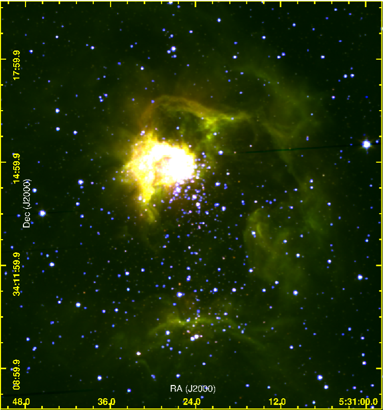
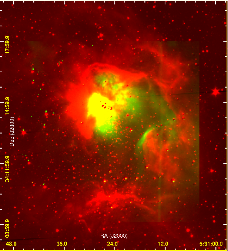
Figure 1.— (left panel:) The color-composite images obtained using the Ks (blue), 3.6 $\mu$m (green) and 4.5 $\mu$m (red) for an area of $\simeq$15 $\times$ 15 arcmin² around NGC 1931. (right panel:) Same as the left panel but using the $H\alpha$ (green) and 3.6 $\mu$m (red) (see the electronic version for the color image).

Table 1 Log of observations.

Date of observation	Filter	Exp. (sec)$\times$ No. of frames
2005 December 31	$B$	$1200\times 3,120\times 1$
	$V$	$900\times 3,60\times 1$
	$I_{c}$	$300\times 2$
	$R_{c}$	$300\times 4$
	$U$	$1800\times 4,300\times 1$
2006 January 22	$I_{c}$	$300\times 4,60\times 3$
2006 January 23	$U$	$300\times 3$
	$B$	$180\times 3,60\times 3$
	$V$	$120\times 3,30\times 3$
	$I_{c}$	$60\times 4,20\times 3$
	$R_{c}$	$60\times 3,20\times 3$
2006 February 24	$H{\alpha}$	$900\times 2,300\times 1$
	$continuum$	$900\times 2,300\times 1$

The photometric data were acquired on 2005 December 31; 2006 January 22, 23; and 2006 February 24, using the 2048 $\times$ 2048 pixel CCD camera mounted on the f/13 Cassegrain focus of the 104-cm Sampurnanand Telescope of Aryabhatta Research Institute of Observational Sciences (ARIES), Nainital, India. In this set up the entire chip covers a field of $\sim$13$\times$13 arcmin² on the sky. The read-out noise and gain of the CCD are 5.3e^- and 10e^-/ADU, respectively. The observations were carried out in the binning mode of 2$\times$2 pixel to improve the signal-to-noise (S/N) ratio. The full width at half-maximum (FWHM) of the star images were $\sim$2$-$3 arcsec. The sky flat frames and bias frames were also taken frequently during the observing runs. A number of short exposures in all the filters were also taken to avoid saturation of bright stars. The observations were standardized using the stars in the SA98 field (Landolt, 1992) observed on 2006 January 23. The log of the observations is given in Table 1. To estimate the contamination due to the foreground/background field stars, a reference field of $\sim$13$\times$13 arcmin² located at about 40$\arcmin$ away, was also observed.

The CCD data frames were reduced using the computing facilities available at ARIES, Nainital. Initial processing of the data frames was done using the IRAF (Image Reduction and Analysis Facility) and ESO-MIDAS (European Southern Observatory Munich Image Data Analysis System) data reduction packages. The details of the data reduction can be found in our earlier works (e.g., Pandey et al., 2007; Jose et al., 2008).

To translate the instrumental magnitudes to the standard magnitudes, the following calibration equations, derived using a least-square linear regression, were used:

$u=U$ + (6.670 $\pm$ 0.011) + (0.044 $\pm$ 0.008)$(U-B)$ + (0.582 $\pm$ 0.013)$X$,
$b=B$ + (4.519 $\pm$ 0.006) + (-0.026 $\pm$ 0.004)$(B-V)$ + (0.332 $\pm$ 0.006)$X$,
$v=V$ + (4.096 $\pm$ 0.004) + (-0.029 $\pm$ 0.003)$(V-I)$ + (0.224 $\pm$ 0.004)$X$,
$r=R_{c}$ + (4.018 $\pm$ 0.006) + (-0.012 $\pm$ 0.007)$(V-R)$ + (0.165 $\pm$ 0.006)$X$,
$i=I_{c}$ +(4.559 $\pm$ 0.006) + (-0.055 $\pm$ 0.003)$(V-I)$ + (0.117 $\pm$ 0.006)$X$

where $U$, $B$, $V$, $R_{C}$ and $I_{C}$ are the standard magnitudes and $u$, $b$, $v$, $r$ and $i$ are the instrumental aperture magnitudes normalized for 1 second of exposure time and $X$ is the airmass. The second-order color correction terms were ignored as they are generally small in comparison to other errors present in the photometric data reduction. The standard deviations of the standardization residuals, $\Delta$, between standard and transformed $V$ magnitude and $(U-B)$, $(B-V)$, $(V-R)$ and $(V-I)$ colors of the standard stars are 0.02, 0.04, 0.02, 0.02 and 0.01 mag, respectively. The typical DAOPHOT errors in magnitude as a function of corresponding magnitude in different passbands are found to increase with the magnitude and become large ($\geq$ 0.1 mag) for stars fainter than V $\simeq$ 21 mag. The measurements beyond this magnitude limit were not considered in the analysis. The photometric data along with positions of the stars are given in Table 2. A sample and format of the Table is shown here. The complete table is available only in electronic form as a part of the online material.

Table 2$UBV(RI)_{C}$ photometric data. The complete table is available in the electronic form.

Star ID	R.A (J2000)	DEC (J2000)	$U\pm\sigma_{U}$	$B\pm\sigma_{B}$	$V\pm\sigma_{V}$	$R_{C}\pm\sigma_{R_{C}}$	$I_{C}\pm\sigma_{I_{C}}$
	(h m s)	($\arcdeg~{}\arcmin~{}\arcsec$)	(mag)	(mag)	(mag)	(mag)	(mag)
(1)	(2)	(3)	(4)	(5)	(6)	(7)	(8)
1	5 30 59.954	34 15 31.95	13.085 $\pm$ 0.007	12.063 $\pm$ 0.005	10.759 $\pm$ 0.006	10.050 $\pm$ 0.008	9.398 $\pm$ 0.013
2	5 31 57.547	34 10 47.45	11.520 $\pm$ 0.007	11.449 $\pm$ 0.008	10.872 $\pm$ 0.009	10.520 $\pm$ 0.002	10.161 $\pm$ 0.009
3	5 31 26.307	34 11 9.94	11.036 $\pm$ 0.005	11.411 $\pm$ 0.009	11.136 $\pm$ 0.010	10.918 $\pm$ 0.005	10.643 $\pm$ 0.005
4	5 31 40.582	34 10 52.00	11.694 $\pm$ 0.006	11.599 $\pm$ 0.009	11.193 $\pm$ 0.011	10.948 $\pm$ 0.005	10.676 $\pm$ 0.007
5	5 31 40.243	34 14 26.25	11.966 $\pm$ 0.008	11.643 $\pm$ 0.006	11.252 $\pm$ 0.012	11.017 $\pm$ 0.006	10.718 $\pm$ 0.010
–	–	—	–	–	–	–	–
–	–	—	–	–	–	–	–
–	–	—	–	–	–	–	–

2.1.1 Completeness of the data

The study of the luminosity functions (LFs)/MFs requires necessary corrections in the data sample to take into account the incompleteness that may occur due to various reasons (e.g. crowding of the stars). We used the ADDSTAR routine of DAOPHOT II to determine the completeness factor (CF). The procedures have been outlined in detail in our earlier works (Pandey et al., 2001, 2005). The CF as a function of $V$ magnitude is given in Table 3, which indicates that present optical data have $\sim$ 90 per cent completeness at $V$ $\sim$ 20 mag. As expected the incompleteness increases with the magnitude.

Table 3Completeness factor (CF) of the optical photometric data in the cluster and field regions.

$V$ range	Cluster region	Field region
(mag)	$r\leq 3.5^{\prime}$
10-11	1.00	1.00
11-12	1.00	1.00
12-13	1.00	1.00
13-14	1.00	1.00
14-15	1.00	1.00
15-16	1.00	1.00
16-17	1.00	0.98
17-18	0.97	0.97
18-19	0.94	0.96
19-20	0.92	0.92
20-21	0.88	0.86

2.1.2 Comparison with previous studies

A comparison of the present photometric data with those available in the literature has been carried out and the difference $\Delta$ (literature - present data) as a function of $V$ magnitude is plotted in Fig. 2. The comparison indicates that the present $V$ mag and colors are in good agreement with the CCD and photoelectric photometry by Pandey & Mahra (1986) and Bhatt et al. (1994), respectively.

Figure 2.— Comparison between the present photometric data with those available in the literature i.e., $\Delta$ (literature$-$present data) as a function of $V$ magnitude. The squares and circles represent the comparison of present data with those by Pandey & Mahra (1986) and Bhatt et al. (1994), respectively.

2.2. Polarimetric data

Polarimetric observations were carried out on two nights (2010 November 12 and 2010 December 13), using the ARIES Imaging Polarimeter (AIMPOL; Rautela, Joshi, & Pandey, 2004) mounted at the Cassegrain focus of the 104-cm Sampurnanand telescope of the ARIES, Nainital, India. The details of the AIMPOL are given in our earlier works (E11 and E12). The observations were carried out in the $V$, $R_{c}$ and $I_{c}$ photometric bands. The detailed procedures used to estimate the polarization and position angles for the program stars are given in E11 and E12.

The instrumental polarization of the AIMPOL is estimated to be less than 0.1 per cent in all the bands (E11, E12). The poarization measurements were corrected for both the null polarization ($\sim$ 0.1 per cent), which is independent of the passbands, and the zero-point polarization angle by observing several unpolarized and polarized standard stars from Schmidt, Elston, & Lupie (1992, here after S92). The results for the polarized standard stars are given in Table 4. The values of $\theta$ are in equatorial coordinate system measured eastwards from the North. Both, the observed degree of polarization [$P(\%)$] and polarization angle [$\theta(\arcdeg)$] for the polarized standards are in good agreement with those given by S92.

Table 4Observed polarized standard stars

	P$\pm\epsilon_{P}$($\%$)	$\theta\pm\epsilon_{\theta}$($\arcdeg$)	P$\pm\epsilon_{P}$($\%$)	$\theta\pm\epsilon_{\theta}$($\arcdeg$)
Our work                               Schmidt et al. (2002)
Polarized standard stars
2010 November 12
HD 19820
$B$	4.54 $\pm$ 0.11	116.3 $\pm$ 0.7	4.70 $\pm$ 0.04	115.7 $\pm$ 0.2
$V$	4.74 $\pm$ 0.10	115.1 $\pm$ 0.6	4.79 $\pm$ 0.03	114.9 $\pm$ 0.2
$R_{c}$	4.57 $\pm$ 0.07	114.4 $\pm$ 0.4	4.53 $\pm$ 0.03	114.5 $\pm$ 0.2
$I_{c}$	3.97 $\pm$ 0.07	115.4 $\pm$ 0.5	4.08 $\pm$ 0.02	114.5 $\pm$ 0.2
HD 204827
$B$	5.75 $\pm$ 0.14	57.6 $\pm$ 0.7	5.65 $\pm$ 0.02	58.2 $\pm$ 0.1
$V$	5.47 $\pm$ 0.10	63.3 $\pm$ 0.5	5.32 $\pm$ 0.01	58.7 $\pm$ 0.1
$R_{c}$	4.93 $\pm$ 0.09	59.2 $\pm$ 0.5	4.89 $\pm$ 0.03	59.1 $\pm$ 0.2
$I_{c}$	4.07 $\pm$ 0.09	59.1 $\pm$ 0.6	4.19 $\pm$ 0.03	59.9 $\pm$ 0.2
2010 December 13
HD 19820
$B$	4.47 $\pm$ 0.11	115.3 $\pm$ 0.7	4.70 $\pm$ 0.04	115.7 $\pm$ 0.2
$V$	4.78 $\pm$ 0.09	115.6 $\pm$ 0.5	4.79 $\pm$ 0.03	114.9 $\pm$ 0.2
$R_{c}$	4.60 $\pm$ 0.07	114.2 $\pm$ 0.4	4.53 $\pm$ 0.03	114.5 $\pm$ 0.2
$I_{c}$	3.99 $\pm$ 0.07	114.3 $\pm$ 0.5	4.08 $\pm$ 0.02	114.5 $\pm$ 0.2
HD 25443
$B$	5.17 $\pm$ 0.11	134.7 $\pm$ 0.6	5.23 $\pm$ 0.09	134.3 $\pm$ 0.5
$V$	5.24 $\pm$ 0.09	134.7 $\pm$ 0.5	5.13 $\pm$ 0.06	134.2 $\pm$ 0.3
$R_{c}$	4.97 $\pm$ 0.09	134.3 $\pm$ 0.5	4.73 $\pm$ 0.05	133.6 $\pm$ 0.3
$I_{c}$	4.27 $\pm$ 0.10	134.6 $\pm$ 0.6	4.25 $\pm$ 0.04	134.2 $\pm$ 0.3

3. Archival data

3.1. 2MASS near-infrared data

NIR $JHKs$ data for point sources in the NGC 1931 region have been obtained from the Two Micron All Sky Survey  (2MASS; Cutri et al., 2003). The 2MASS data reported to be 99% complete up to $\sim$ 15.7, 15.1, 14.3 mag in $J$, $H$, $K_{s}$ bands, respectively. To ensure photometric accuracy, we used only those photometric data which have quality flag ph-qual=AAA, which endorses a S/N $\geq$ 10 and photometric uncertainty $\textless$ 0.10 mag. The NIR data are used to identify the classical T-Tauri stars (CTTSs) and weak line T-Tauri stars (WTTSs).

3.2. Spitzer IRAC data

The archived MIR data observed with the Spitzer Infrared Array Camera (IRAC) have also been used in the present study. We obtained basic calibrated data (BCD) using the software Leopard. The exposure time of each BCD was 10.4 sec and for each mosaic, 169 and 139 BCDs respectively, in Ch1 (3.6 $\mu$m) and Ch2 (4.5 $\mu$m) have been used. Mosaicking was performed using the MOPEX software provided by Spitzer Science Center (SSC). All of the mosaics were built at the native instrument resolution of 1.2 arcsec pixel^-1 with the standard BCDs. In order to avoid source confusion due to crowding, PSF photometry for all the sources was carried out using the DAOPHOT package available with the IRAF photometry routine. The detections are also examined visually in each band to remove non-stellar objects or false detections. The sources with photometric uncertainties $\textless$ 0.2 mag in each band were considered as good detections. A total of 3950 and 2793 sources were detected in the 3.6 and 4.5 $\mu$m bands. Aperture photometry for well isolated sources was done using an aperture radius of 3.6 arcsec with a concentric sky annulus of the inner and outer radii of 3.6 and 8.4 arcsec, respectively. For a standard aperture radius (12 arcsec) and background annulus of 12$-$22.4 arcsec, we adopted zero-point magnitude as 19.670 and 18.921 for the 3.6 and 4.5 $\mu$m bands, respectively. Aperture corrections were also made using the values described in the IRAC Data Handbook (Reach et al. 2006). The necessary aperture correction for the PSF photometry was then calculated from the selected isolated sources and were applied to the PSF magnitudes of all the sources.

4. STRUCTURE OF THE CLUSTER

Chen et al. (2004) and Sharma et al. (2006) have found that the initial stellar distribution in star clusters may be governed by the structure of the parental molecular cloud as well as how star formation proceeds in the cloud. Later evolution of the cluster may be governed by internal gravitational interaction among member stars and by external tidal forces due to the Galactic disk or giant molecular clouds.

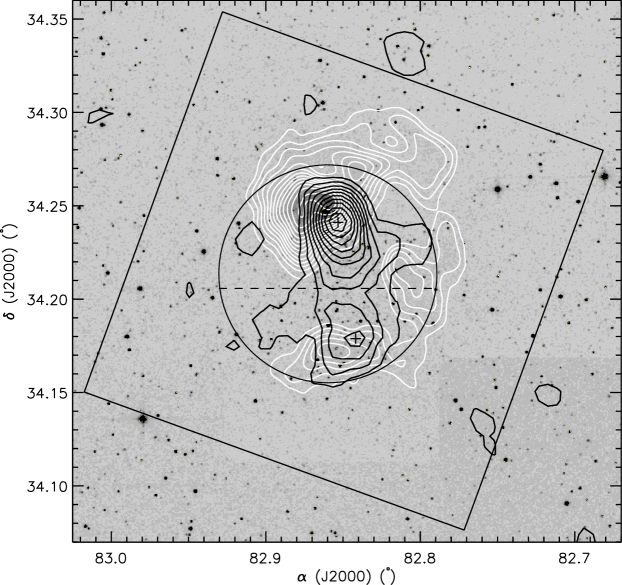
Figure 3.— The isodensity contours (thick black curves) generated from the 2MASS $K_{s}$-band data (with $\sigma_{K_{s}}\textless$ 0.1 mag) using a grid size of $\simeq$35 $\times$ 35 arcsec². The contours are plotted above 1$\sigma$ level. The contours have a step size of 2 stars/arcmin² with the lowest contour representing 5 stars/arcmin². Isodensity contours manifest two prominent clusterings. The dashed line demarcates northern and southern parts of the region. The thick white contours represent the MSX A-band (8.3 $\mu$m) intensity distribution. The minimum and maximum contour levels of the MSX A-band intensity are 1.78$\times$10^-6 W/m²-Sr and 3.35$\times$10^-5 W/m²-Sr, respectively. The area marked with the continuous line represents the region covered by optical photometry. The circle represents the estimated boundary of the region. The plus sign represents the center of the clusters.

The isodensity contours shown in Fig. 3, obtained using the stars detected in the 2MASS $K_{s}$-band ($\sigma_{Ks}\textless$ 0.1 mag), are used to study the morphology of the cluster. The contours are plotted above 1$\sigma$ level. The surface density distribution reveals two prominent structures distributed around $\alpha$(2000)=05^h31^m24$\fs$781, $\delta$(2000)=+34$\arcdeg$14$\arcmin$28$\farcs$05 and $\alpha$(2000)=05^h31^m22$\fs$034, $\delta$(2000)=+34$\arcdeg$10$\arcmin$43$\farcs$99, suggesting the presence of a double cluster in the region. In fact the radial density profile (RDP) of the region by Bonatto & Bica (2009) also reveals a density enhancement around the radial distance of $\sim$ 3$-$5 arcmin.

We used the star count technique to estimate the radial extent of the two clusters. The points of maximum densities in Fig. 3 were considered as the center of the clusters. The RDP is derived using the 2MASS $K_{s}$-band data ($\sigma_{K_{s}}~{}\textless$ 0.1 mag) by dividing star counts inside the concentric annulus of 30 arcsec width around the cluster center by the respective area. The densities thus obtained are plotted as a function of radius in Fig. 4, where, 1 arcmin at the distance of the cluster (2.3 kpc, cf. Section 6.1) corresponds to $\sim$ 0.67 pc. The upper and lower panels show the RDPs for the northern and southern clusters, respectively. The error bars are derived assuming that the number of stars in each annulus follows Poisson statistics.

Figure 4.— The radial density profile (RDP) is derived using the 2MASS $K_{s}$-band data (using $\sigma_{K_{s}}~{}\textless$ 0.1) by dividing star counts inside the concentric annulus of 30 arcsec width around the cluster center by the respective area. The densities thus obtained are plotted as a function of radius. The upper and lower panels show the RDPs for the northern and southern clusters respectively.

The radial extent of the clusters ($r_{cl}$) is defined as the point where the cluster stellar density merges with the field stellar density. Within the errors, the observed RDPs for both the clusters seem to merge with the background field at a radial distance of $\sim$ 2 arcmin. Hence, we assume a radius of 2 arcmin for both the clusters.

5. ANALYSIS OF THE POLARIMETRIC DATA

5.1. Polarization vector map & Distribution of $P_{V/R/I}$ $(\%)$ and $\theta_{V/R/I}$ $(\arcdeg)$

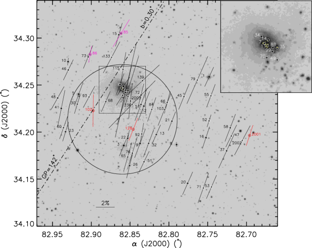
Figure 5.— The polarization measurements of the stars in NGC 1931 are superimposed on the 2MASS $K_{s}$-band image. The stars with $V$-band polarimetric measurements are shown with black vectors. The red and magenta vectors represent polarimetric measurements in $R_{C}$ and $I_{C}$-bands. The dashed-dotted line represents the orientation of the projection of the GP at $b=0\fdg 30$ which corresponds to a position angle of 142$\arcdeg$. A vector with a 2 per cent of polarization at a position angle of 90$\arcdeg$ is drawn for a reference. Barring a few vectors near the cluster center (shown in a square box), the majority of the vectors are closely aligned with GP indicating an ordered magnetic field towards NGC 1931. The vectors in the nebulous region of the cluster show a scattered distribution. Two stars #139 and #236 show high degree of polarization as well as different polarization angles from the rest of the stars. These stars are identified as probable YSOs (cf. Sec 6.2.3). The box at the corner shows an enlarged view of the central region. See the electronic version for the color image.

Table 6 lists the polarization measurements for 62 stars towards the cluster region. The star identification numbers for 59 stars are taken from column 1 of Table 2, whereas three stars #2001, #2002 and #2003, do not have optical data. The degree of polarization P (in per cent), polarization angles $\theta$ (in degree) measured in $V,(R,I)_{c}$ bands and their corresponding standard errors are given in columns $4-9$. The black vectors (Fig. 5) show the sky projection of the $V$-band polarization measurements. In the case of a few stars for which the $V$-band polarization measurements are not available, we plotted the polarization measurements either of $R_{c}$-band (red) or $I_{c}$-band (magenta). The length of each polarization vector is proportional to the degree of polarization. The dashed-dotted line represents the orientation of the projection of the Galactic plane ($GP$) at $b$ = 0.30$\arcdeg$, which corresponds to a position angle of 142$\arcdeg$. Interestingly, all the polarization vectors except those near the cluster center (enclosed by a square box) are roughly parallel to the GP. The enlarged view of the central region is shown in a separate panel at the top right part of the figure. The polarization measurements of two stars #7 and #11 could be affected by their close companions as well as by the nebulosity. Hence, the polarization measurements of these stars could be less reliable.

Figure 6.— Frequency distribution of polarization (left panel) and polarization angle values (right panel) for the stars detected in $V,(R,I)_{c}$ bands. In each case, the mean and standard deviation of polarization and polarization angle values are obtained by fitting a Gaussian function. The number of sources detected in each passband is also indicated. The position angle corresponds to the $b=0.30\arcdeg$ (GP) is also shown at 142$\arcdeg$ with a thick line. The mean polarization angles differ from the GP by $\sim$13$\arcdeg$.

The distribution of $P$ and $\theta$ in $V,(R,I)_{c}$ bands is shown in Fig. 6. A Gaussian fit to the each distribution yields a mean and a standard deviation as $P_{V}=2.4\pm$0.6 per cent, $P_{R}=2.2\pm$0.5 per cent, $P_{I}=2.0\pm$0.6 per cent, and $\theta_{V}=155\pm 7\arcdeg$, $\theta_{R}=154\pm 6\arcdeg$, $\theta_{I}=156\pm 12\arcdeg$. The values of $P_{V}(2.4\pm 0.6$ per cent) and $\theta_{V}(155\pm 7\arcdeg)$ towards NGC 1931 are comparable to those ($P_{V}=2.3\pm$0.1 per cent and $\theta_{V}=160\pm 3\arcdeg$, E11) for Stock 8 (${\it l}=173.37\arcdeg$, $b=-0.18\arcdeg$, distance = 2.05 kpc) which is spatically located near the NGC 1931.

5.2. Member identification

The identification of probable members of a cluster and the foreground/background stars towards the direction of the cluster is necessary to study the nature of the dust properties of the ICM/ISM and the magnetic field associated with the foreground and the ICM. Our earlier studies (E11 & E12) have shown that the polarimetry in combination with the $(U-B)-(B-V)$ two-color diagram (TCD) can be efficiently use to identify the probable members in the cluster region. This section describes the determination of membership using the polarization properties in combination with the $(U-B)-(B-V)$ TCD.

Figure 7.— $U$ versus $Q$ diagrams for all the stars given in Table 6. Open circles represent the stars having $V$-band data. The filled squares represent the stars located within the box as shown in Fig 5. The triangles represent the stars having either single or double band polarimetric data. The box with dashed line marks the boundary of mean $P\pm\sigma$ and mean $\theta\pm\sigma$. The position of the Sun is also shown with a square box at the ($Q=0$, $U=0$) coordinates. The GP is drawn with a dotted line. The stars distributed within or nearby 1$\sigma$ box of all the three Stokes planes are considered as probable members associated with the cluster.

The individual Stokes parameters of the polarization vectors of the V/R/I-band, $P_{V/R_{c}/I_{c}}$, given by $Q_{V/R_{c}/I_{c}}$ = $P_{V/R_{c}/I_{c}}$ $\cos$(2$\theta_{V/R_{c}/I_{c}}$) and $U_{V/R_{c}/I_{c}}$ = $P_{V/R_{c}/I_{c}}$ $\sin$(2$\theta_{V/R_{c}/I_{c}}$) have been estimated and are presented in the $U_{V/R_{c}/I_{c}}$ versus $Q_{V/R_{c}/I_{c}}$ plot as shown in Fig. 7. Since the polarization of light from a star depends on the column density of aligned dust grains that lie in front of the star, the cluster members are expected to group together in the $U$ versus $Q$ plot, whereas non-members are expected to show a scattered distribution. Similarly, the polarization angles of cluster members would be similar but could be different for foreground or background non-member stars as light from them could be affected in a different manner because of contributions from different/additional dust components. Therefore, the $U-Q$ plot is a useful tool to segregate the members from non-members in the cluster region. However, the stars with intrinsic polarization, e.g., due to an asymmetric distribution of matter around YSOs and/or rotation in their polarization angles (see e.g., E11 & E12), may also create scattered distribution in the $U-Q$ plane.

The probable members of the cluster should have a similar location in all the three $U-Q$ diagrams. The Stokes parameters for the stars lying within the square box as shown in Fig. 5 and embedded in the nebulosity are shown with filled squares. The box with dashed line in $U-Q$ plots shows the boundary of the area having mean P $\pm$ $\sigma$ ($P_{V}$=2.4$\pm$0.6 per cent, $P_{R}$=2.3$\pm$0.5 per cent, $P_{I}$=2.0$\pm$0.6 per cent) and mean $\theta$ $\pm$ $\sigma$ ($\theta_{V}$=155$\arcdeg\pm 7\arcdeg$, $\theta_{R}$=155$\arcdeg\pm 6\arcdeg$, $\theta_{I}$=156$\arcdeg\pm 12\arcdeg$) obtained from the distribution shown in Fig. 6. The stars lying within or near the 1$\sigma$ box in all the three $U-Q$ plots may be probable members associated with the cluster.

Figure 8.— $(U-B)$ versus $(B-V)$ TCD of the stars with polarimetric data. The symbols are the same as in the Fig. 7. The ZAMS from Schmidt-Kaler (1982) is shifted along a normal reddening vector having a slope of $E(U-B)/E(B-V)$ = 0.72. The TCD shows a variable reddening in the cluster region with $E(B-V)_{min}$ $\sim$ 0.5 mag and $E(B-V)_{max}$ $\sim$ 0.9 mag.

It is expected that the members of a cluster should exhibit comparable $E(B-V)$ values, whereas the foreground (background) population is expected to be less (highly) extincted as compared to the cluster members. Fig. 8 shows the $(U-B)-(B-V)$ TCD for only 58 stars as $U-B$ color is not available for three stars. The symbols of the stars are same as in Fig. 7. All the stars shown in Fig. 8 have the polarimetric data. In Fig. 8, the zero-age main sequence (ZAMS) from Schmidt-Kaler (1982) is shifted along a normal reddening vector having a slope of $E(U-B)/E(B-V)$ = 0.72. The TCD shows a variable reddening in the cluster region with $E(B-V)_{min}$ $\sim$ 0.5 mag and $E(B-V)_{max}$ $\sim$ 0.9 mag. It is also apparent from Fig. 8 that sources located in the northern nebulous region (lying within the box in Fig. 5) reveals presence of parent molecular cloud and show a variable extinction of $E(B-V)$ $\sim$ $0.5-0.9$ mag. The polarimetric observations in combination with the $(U-B)-(B-V)$ $TCD$ are used to identify members of the NGC 1931 cluster (cf. E11 and E12). The probable members thus identified are given in Table 5. The stars #7, 11, 14, 35, 49, 88 and 99 are embedded in the northern nebulosity, hence the polarization measurements may be affected by the nebulosity, consequently may show scattered distribution in the $U$ vs $Q$ diagram. Out of 22 probable members, 11 stars (#3, 7, 11, 14, 21, 22, 35, 49, 79, 88 and 93) have either $\sigma_{1}\textgreater$ 1.5 and/or $\overline{\epsilon}\textgreater$ 2.3, indicating for the presence of intrinsic polarization and/or rotation in their polarization angles (cf. Sec 5.4).

Table 5The list of probable members of the cluster selected on the basis of polarimetric and photometric observations.

Star ID	$E(B-V)$	lying within 3$\farcm$5 region
	(mag)
3	0.47	yes
5	0.38	yes⋆
7	0.61	yes†
9	0.46	yes
11	0.79	yes†
12	0.54	yes
13	0.52	yes
14	0.75	yes†
21	0.36	yes⋆
22	0.48	yes
32	0.70	yes
35	0.91	yes†
45	0.75	no
47	0.59	no
49	0.64	yes†
51	0.51	yes
53	0.69	no
55	0.44	no
79	0.59	no
88	0.80	yes†
93	0.92	yes
99	0.62	yes†

$\star$: The polarization of these sources is comparable to the cluster members, however the $E(B-V)$ values for these stars are less than minimum reddening ($E(B-V)_{min}$=0.50 mag) for the cluster region.
$\dagger$: These stars are embedded in the northern nebulosity.

5.3. Dust distribution

Figure 9.— $U_{V}$ versus $Q_{V}$ plot of the 10 probable cluster members of NGC 1931, which are free from possible intrinsic polarization and polarization angle rotation and also free from background nebulosity, along with other clusters towards the direction of NGC 1931. The data for other clusters have been taken from E11.

In our previous studies (E11 and E12) we have shown that the Stokes plane can be used to study the distribution of dust layers, the role of dust layers in polarization, the associated magnetic field orientation, etc. The vector connecting two points in the Stokes plane represents the amount of polarization, whereas the change in the direction of vectors indicates a change in the polarization angle. In the case of uniformly aligned dust grains (i.e. uniform magnetic field orientation), the degree of polarization is expected to increase with distance, but the direction of polarization (polarization angle) should remain the same and hence the Stokes vector should not change its direction with increasing distance. For example, in the case of NGC 1893 (E11), the degree of polarization was found to increase with distance, whereas the direction of polarization remained almost constant (cf. their figure 5). In contrast, the magnetic field orientation shows systematic rotation with distance towards the direction of Berkeley 59 (E12, see their figure 7) as the radiation from the cluster members might have a depolarization effect due to the systematic change in the dust grain alignment in the foreground medium. NGC 1931 is located towards the direction of NGC 1893 hence a similar behavior is expected for the cluster NGC 1931 also. Fig. 9 shows the $U_{V}-Q_{V}$ distribution for probable members of NGC 1931 along with the data for other clusters NGC 2281 ($\sim$ 0.6 kpc), NGC 1664 ($\sim$ 1.2 kpc), NGC 1960 ($\sim$ 1.3 kpc), Stock 8 ($\sim$ 2.0 kpc), NGC 1893 ($\sim$ 3.2 kpc), located towards the direction of NGC 1931. The data for other clusters have been taken from E11. Out of 22 probable members (cf. Table 5) of NGC 1931, we have used only 10 stars (#5, 9, 12, 13, 32, 45, 47, 51, 53 and 55) in Fig. 9 which are free from intrinsic polarization and/or rotation in their polarization angles and also free from the background nebulosity. The polarization data for NGC 1931 is consistent with the fact that the degree of polarization increases with the column density of dust grains lying in front of the stars that are relatively well aligned.

The various dust layers located between the star and the observer can cause a sudden increase in degree of polarization. The number of such sudden increase has been used by E11 to characterize the dust layers encountered by the radiation along its path and the relative magnetic field orientations of the dust layers towards the direction of NGC 1893 which is spatially located near the cluster NGC 1931. The polarimetric observations for NGC 1931 obtained in the present study follow the general trend revealed by the stars and clusters located towards the anticenter direction of the Galaxy as described by E11.

5.4. Dust properties

The wavelength dependence of polarization in the Galaxy can be represented by the following relation (Serkowski, 1973; Coyne, Gehrels, & Serkowski, 1974; Wilking, Lebofsky, & Rieke, 1982);

$$P_{\lambda}=P_{max}~{}\exp[-K~{}ln^{2}(\lambda_{max}/\lambda)]\\$$ (1)

where $P_{\lambda}$ and $\lambda_{max}$ are the percentage polarization at wavelength $\lambda$ and the peak polarization, occurring at wavelength $\lambda_{max}$. The $\lambda_{max}$ depends on the optical properties and characteristic particle size distribution of aligned grains (Serkowski, Mathewson, & Ford, 1975; McMillan, 1978) whereas the value of $P_{max}$ is dictated by the chemical composition, shape, size, column density, and alignment efficiency of the dust grains. The Serkowski’s relation with $K$=1.15 provides a reasonable representation of the observations of interstellar polarization between wavelengths 0.36 and 1.0 $\mu$m. The $P_{max}$ and $\lambda_{max}$ are obtained using the weighted least-squares fitting to the measured polarization in $V(RI)_{c}$ bands to equation 1 by adopting $K$=1.15. The parameters $\sigma_{1}$ (the unit weight error of the fit for each star), which quantifies the departure of the data from the standard Serkowski’s law, and $\overline{\epsilon}$, the dispersion of the polarization angle for each star normalized by the average of the polarization angle errors (cf. Marraco et al., 1993) were also estimated. The estimated values of $P_{max}$, $\lambda_{max}$, $\sigma_{1}$ and $\overline{\epsilon}$ for each star are given in Table 6.

Figure 10.— (upper panel): $\sigma_{1}$ versus $P_{max}$ and (lower panel): $\overline{\epsilon}$ versus $\lambda_{max}$. Stars with $\sigma_{1}\textgreater$ 1.5, $\overline{\epsilon}$ $\textgreater$ 2.3 and with $\lambda_{max}$ $\textless$ 0.35$\mu$m (#34) are marked with their IDs. The symbols are same as in Fig. 7

Fig. 10 shows $\sigma_{1}$ versus $P_{max}$ (upper panel) and $\overline{\epsilon}$ versus $\lambda_{max}$ (lower panel) plots. The criteria mentioned above indicate that majority of the stars do not show evidence of intrinsic polarization. However, a few stars (15) show indication of either intrinsic polarization and/or rotation in their polarization angles. Ten stars (#3, 14, 15, 21, 22, 26, 35, 88, 93 and 139) are found to exhibit an indication of intrinsic polarization as they have $\sigma_{1}$ $\textgreater$ 1.5 and 8 stars (7, 11, 15, 35, 49, 79, 88 and 139) are found to show rotation in their polarization angles, whose $\overline{\epsilon}$ values are higher ($\textgreater$ 2.3) than that for the rest of the stars. Four stars (15, 35, 88 and 139) are found to show both indication of intrinsic polarization and also rotation in their polarization angles.

The weighted mean values of $P_{max}$ and $\lambda_{max}$ using all the 22 probable members are found to be 2.51$\pm$ 0.03 per cent and 0.57$\pm$ 0.01 $\mu$m, respectively. Exclusion of stars showing intrinsic polarization does not change the mean values of $P_{max}$ and $\lambda_{max}$ significantly. The estimated $\lambda_{max}$ is slightly higher than the value corresponding to the diffuse ISM  (0.545 $\mu$m; Serkowski et al., 1975). Using the relation $R_{V}$=(5.6$\pm$0.3)$\times$ $\lambda_{max}$  (Whittet & van Breda, 1978), the value of $R_{V}$, the total-to-selective extinction, comes out to be 3.20 $\pm$ 0.05.

However the $\lambda_{max}$ value (0.55$\pm$0.01$\mu$m; E11) towards the cluster NGC 1893, which is spatially close to NGC 1931, is found to be comparable to the value for the diffuse ISM (0.545$\mu$m; Serkowski et al. 1975) as well as the reddening law towards NGC 1893 is found to be average (Sharma et al., 2007). This indicates that size of the dust grains towards NGC 1893 is comparable to those in the diffuse ISM. Jose et al. (2008) have also found the presence of average reddening law towards the cluster region of Stock 8 which is also located near the NGC 1931. The indication of slightly bigger dust grains towards NGC 1931 could be due to relatively bigger dust grains within the “intra-cluster medium”. The extinction law in the cluster region is further discussed in the ensuing section.

5.5. Extinction law

Figure 11.— The TCDs of the form $(V-\lambda)$ vs. $(B-V)$, where $\lambda$ is $I$, $J$, $H$ or $K_{s}$. Only the probable cluster members identified on the basis of polarimetric data, photometric color-color diagrams and color-magnitude diagrams have been used (cf. Sec 5.2). The open circles and triangles represent the stars having $V(RI)_{C}$ and single or double band polarimetric data, respectively. The star symbols are the probable PMS stars (cf. Sec 6.2.3). The filled square symbols are the stars lying in the northern nebulous region. The slopes of the straight line fit are indicated on right hand side of each panel. The stars in the nebulous region (filled square symbols) and two (# 88 and # 236) PMS stars are not used in the fit.

The $(V-\lambda)$ vs. $(B-V)$ TCDs, where $\lambda$ is one of the wavelengths of the broadband filters $R,I,J,H,K$ or $L$, have been used to separate the influence of the extinction produced by the diffuse ISM from that of the extinction due to the ICM (cf. Chini & Wargau, 1990; Pandey et al., 2000). The ($V-\lambda$) vs. ($B-V$) TCDs for the probable members (selected on the basis of polarimetric analysis and optical color-color diagrams; cf. Sec 5.2) and probable PMS stars (cf. Sec. 6.2.3) of the cluster region are shown in Fig. 11. The open circles are the stars with $V(RI)_{C}$ polarimetric data and the triangles are those with either single or double band polarimetric data. The slope for the general distribution of majority of the stars (excluding the stars in the nebulous region (filled square symbols) and two (# 88 and # 236) PMS stars) is found to be 1.17$\pm$0.05, 2.10$\pm$0.12, 2.63$\pm$0.14 and 2.76$\pm$0.16 for $(V-I)$, $(V-J)$, $(V-H)$, $(V-K)$ versus $(B-V)$ TCDs respectively. These slopes are higher in comparison to those obtained for diffuse ISM, which indicates a differing reddening law in the cluster region. The stars associated with the nebulous region of the northern cluster, shown with filled square symbols, seems to be deviate from the distribution of the majority of the stars.

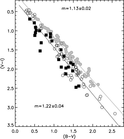
Figure 12.— The $(V-I)$ vs. $(B-V)$ TCD for the stars distributed in the cluster region. The gray filled circles are considered as field stars, whereas those shown with open circles are considered as probable cluster members. The stars distributed in the northern nebulous part of the cluster are shown with filled squares. The slopes of the gray and black continuous straight line fits to the field (1.13$\pm$0.03) and probable cluster members (1.22$\pm$0.04), respectively, are also indicated.

To have a general view of the reddening law in the cluster region ($r$ $\leq$ 3.5 arcmin), we used TCDs for all the sources detected in the region. Fig. 12 shows $(V-I)$ vs. $(B-V)$ TCD which indicates a combination of distributions for the field stars and the cluster members. We selected probable field stars visually assuming that stars following the slope of the diffuse ISM are contaminating field stars in the cluster region, and they are shown by gray filled circles. The slopes for the diffuse ISM have been taken from  Pandey et al. (2003). The remaining sources shown by open circles may be probable members of the cluster. The probable members associated with the nebulous region are shown by filled squares. The slopes of the distributions for probable cluster members (i.e. open circles + filled squares), $m_{cluster}$ are found to be 1.22$\pm$0.04, 2.20$\pm$0.08, 2.67$\pm$0.10, 2.81$\pm$0.12, for the $(V-I)$, $(V-J)$, $(V-H)$, $(V-K)$ vs. $(B-V)$ TCDs respectively. The ratios $E(V-\lambda)/E(B-V)$ and the ratio of total-to-selective extinction for the general distribution of probable cluster members in the cluster region, $R_{cluster}$, is derived using the procedure given by  Pandey et al. (2003). Assuming the value of $R_{V}$ for the diffuse foreground ISM as 3.1, the ratios $E(V-\lambda)/E(B-V)$ yield $R_{cluster}$ = 3.3$\pm$0.1, which is in fair agreement with the value derived using polarimetric data (cf. Sec 5.4) and indicate a differing reddening law in the cluster region. The probable members associated with the nebulous region, shown by filled squares, indicate a relatively higher $R_{V}$ value for the nebulous region. Several studies e.g. Pandey et al. (2003), Pandey et al. (2008) and references therein, have pointed out a high $R_{V}$ values in the vicinity of star-forming regions, which is attributed to the presence of larger dust grains in the region.

5.6. Polarization efficiency

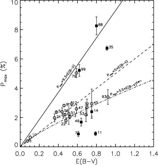
Figure 13.— $P_{max}$ versus $E(B-V)$ diagram. The symbols are the same as in Fig. 7. The continuous line represents the empirical upper limit relation for the polarization efficiency (assuming $R_{V}$= 3.1) of $P_{max}=9.3\times E(B-V)$ (Serkowski et al., 1975). The dashed line represents the relation $P_{max}=5\times E(B-V)$ (Serkowski et al., 1975) and the dashed-dotted line represents the relation $P_{max}$ = 3.5 $\times$ $E(B-V)^{0.811}$ by Fosalba et al. (2002).

The polarization efficiency [$P_{max}/E(B-V)$] of the medium depends mainly on the magnetic field strength, the grain alignment efficiency and the amount of depolarization due to the radiation passing through various mediums having different magnetic field directions (see e.g. Feinstein et al., 2003, E11 & E12 and references therein). Figure 13 displays the polarization efficiency diagram for the stars towards NGC 1931. The empirical upper limit relation for the polarization efficiency of the diffuse ISM, given by $P_{max}=3A_{V}\simeq 3R_{V}E(B-V)\simeq 9.3E(B-V)$  (assuming $R_{V}$=3.1, Hiltner & Johnson, 1956; Serkowski et al., 1975), shown by a continuous line in Fig. 13. Serkowski et al. (1975) have shown that the polarization efficiency of the ISM in general follows a mean relation $P_{max}\simeq 5E(B-V)$ and the same is shown by a dashed line. The dashed-dotted line represents the average polarization efficiency for the general diffuse ISM by Fosalba et al. (2002), which is valid for $E(B-V)$ $\textless$ 1.0 mag. The majority of the cluster members are distributed below the dashed line indicating that polarization efficiency of the ICM is less than the polarization efficiency of the diffuse ISM ($\sim$5 per cent per mag) and seems to follow the relation for the general diffuse ISM by Fosalba et al. (2002). Four stars, #35, #79, #88 and #99 have relatively high polarization ($P_{max}$ $\sim$ 5 to 8 per cent) and polarization efficiency greater than 5 per cent per mag. Interestingly, the stars #35 and #88 have $\sigma_{1}$ and $\overline{\epsilon}$ values $\textgreater$ 1.5 and $\textgreater$ 2.3 respectively, thereby indicating presence of intrinsic polarization and rotation in their polarization angles. It is worthwhile to mention that these two stars are associated with the nebulosity of the northern region. The star #79 has $\overline{\epsilon}$ $\textgreater$ 2.3 which indicates a rotation in the polarization angle. The stars #7 and #11 show significantly smaller polarization efficiency ($\sim$ 1 per cent per mag). The $\overline{\epsilon}$ values for these stars are $\textgreater$ 2.3, hence there could be a rotation in the polarization angle. As we have already mentioned (cf. Sec 5.1), the polarization measurements of these two stars (#7 and #11) are less reliable. Interestingly, all the stars deviating from the mean polarization efficiency behavior of the region are located in the northern region.

Here it is interesting to mention that the dust grains towards NGC 1893 ($l=173\fdg 6,b=-1\fdg 7$), which is spatially close to NGC 1931, show higher polarization efficiency (cf. figure 9, E11) whereas the the dust grains towards NGC 1931 exhibit less polarization efficiency in comparison to mean polarization efficiency for the general diffuse ISM. This could be due to the average extinction law in the foreground medium and differing reddening law in the intra-cluster medium.

6. STELLAR CONTENTS OF THE CLUSTER

6.1. Optical color-magnitude diagram: Distance and Age

Figure 14.— De-reddened $V$ versus $(B-V)$ CMD for probable member stars (cf. Sec. 5.2). The post main-sequence isochrones for 1 Myr (Z=0.02) by Marigo et al. (2008) has been plotted after correcting for the distance and reddening. The average error in color is shown in the right side of the figure. The polarization of two sources #5 and #21 is comparable to the cluster members, however the $E(B-V)$ values for these stars are less than the minimum reddening ($E(B-V)_{min}$=0.50 mag) for the cluster region (cf. Table 5).

The $V_{0}/(B-V)_{0}$ color-magnitude diagram (CMD; Fig. 14) of the identified 22 probable members (Sec 5.2) has been used to estimate the distance to the cluster. Reddening of individual probable members having spectral types earlier than $A0$ has been estimated using the reddening free index Q (Johnson & Morgan, 1953) which is defined as $Q=(U-B)-0.72(B-V)$. The reddening law was assumed to be normal. The intrinsic $(B-V)_{0}$ color and color-excess for the MS stars can be obtained from the relation $(B-V)_{0}$ = 0.332$\times$Q  (Johnson, 1966; Hillenbrand et al., 1993) and $E(B-V)=(B-V)-(B-V)_{0}$, respectively. A visual fit of the isochrone for 1 Myr and Z=0.02 by Marigo et al. (2008) to the observations yields a distance modulus of $V_{0}-M_{V}$=11.81$\pm$0.3 which corresponds to a distance of 2.3$\pm$0.3 kpc. The distance estimate is in agreement with that obtained by Pandey & Mahra (1986); Bhatt et al. (1994); Bonatto & Bica (2009).

Stars #7 ($E(B-V)$ =0.61) and #11 ($E(B-V)$ = 0.79) are located in the northern nebulous region and could be the ionizing source(s) of the region (cf. Sec 8). The star #3 is located in the southern region and has $E(B-V)$ =0.47. The present photometric data for star #3 is in agreement with that reported by Moffat et al. (1979). The $E(B-V)$ value for star #3 is comparable to the $E(B-V)_{min}$. Moffat et al. (1979) concluded that either this star is a foreground star or could be a binary star. Since polarimetric observations suggest that it could be a member, we presume that this star could be binary star and a member of the cluster.

Figure 15.— The $V/(V-I)$ CMDs for all the stars within $r_{cl}~{}\leqslant~{}3.5\arcmin$ of the cluster region (left panel), the nearby field region (middle panel) and statistically cleaned $V/(V-I)$ CMD (right panel).

The $V/(V-I)$ CMDs of all the stars within the cluster region (i.e. $r_{cl}~{}\leqslant~{}3.5\arcmin$) and the nearby field region are shown in the left and middle panels of Fig. 15. As discussed in our earlier works (e.g., Pandey et al., 2008; Jose et al., 2008) the removal of field star contamination from the sample of stars in the cluster region is necessary as both PMS and dwarf foreground stars occupy similar positions above the ZAMS in the CMDs. Since proper-motion data is not available for the region, the statistical criterion was used to estimate the number of probable member stars in the cluster region. To remove contamination due to field stars, we statistically subtracted their contribution from the CMD of the cluster region using the following procedure. The CMDs of the cluster as well as of the reference region were divided into grids of $\Delta{V}=1$ mag and $\Delta(V-I)$ = 0.4 mag. The number of stars in each grid of the CMDs were counted. After applying the completeness corrections using the CF (cf. Table 3) to both the data samples, the probable number of cluster members in each grid were estimated by subtracting the corrected reference star counts from the corrected counts in the cluster region. The estimated numbers of contaminating field stars were removed from the cluster CMD in the following manner. For a randomly selected star in the CMD of the reference region, the nearest star in the cluster CMD within $V\pm 0.25$ and $(V-I)\pm 0.125$ of the field was removed. Although the statistically cleaned $V/(V-I)$ CMD of the cluster region shown in the right panel of Fig. 15 clearly shows the presence of PMS stars in the cluster, however the contamination due to field stars near $V$ $\sim$ 20 mag and $(V-I)$ $\sim$ 2.0 can still be seen (cf. Fig. 16). This field population could be due to the background population as discussed by Pandey et al. (2006).

Figure 16.— The statistically cleaned CMD for the region within the 3.5 arcmin radius (cf. Fig. 3). The average error in $V$ and $(V-I)$ colors are shown in the right side of the figure.

The statistically cleaned $V/(V-I)$ CMD (SCMD) of the cluster region with PMS isochrones by Siess et al. (2000) for ages 1, 2, 5 and 10 Myr (dashed curves) and 1 Myr (continuous curve) by Marigo et al. (2008) is shown in the Fig. 16 which manifests the presence of PMS population with an age spread of $\sim$ 5 Myr. The statistics of PMS sources obtained from the SCMD can be used to study the initial mass function ($IMF$) of PMS population of NGC 1931. Here we would like to point out that the points shown by filled circles in Fig. 16 may not represent the actual members of the clusters. However, the filled circles should represent the statistics of PMS stars in the region and it has been used to study the $MF$ of the cluster region.

6.2. Identification of YSOs

6.2.1 On the basis of $(J-H)/(H-K)$ TCD

NIR imaging surveys are important tools to detect YSOs in star forming regions. The locations of YSOs on $(J-H)/(H-K)$ two-color diagram (NIR TCD) are determined to a large extent by their evolutionary state. The NIR TCD using the 2MASS data for all the sources lying in the NGC 1931 region and having photometric errors less than 0.1 magnitude is shown in the left panel of Fig. 17. All the 2MASS magnitudes and colors have been converted into the California Institute of Technology (CIT) system. The solid and thick dashed curves represent the unreddened MS and giant branch (Bessell & Brett, 1988), respectively. The dotted line indicates the locus of unreddened TTSs (Meyer et al., 1997). All the curves and lines are also in the CIT system. The parallel dashed lines are the reddening vectors drawn from the tip (spectral type M4) of the giant branch (left reddening line), from the base (spectral type $A0$) of the MS branch (middle reddening line) and from the tip of the intrinsic TTS line (right reddening line). The extinction ratios $A_{J}/A_{V}=0.265,A_{H}/A_{V}=0.155$ and $A_{K}/A_{V}=0.090$ have been taken from Cohen et al. (1981). The sources located in the ‘F’ region (cf. left panel of Fig. 17) could be either field stars (MS stars, giants) or Class III and Class II sources with small NIR-excesses, whereas the sources distributed in the ‘T’ and ‘P’ regions are considered to be mostly Classical TTSs (CTTSs or Class II objects) with relatively large NIR-excesses and likely Class I objects, respectively (for details see Pandey et al., 2008; Chauhan et al., 2011a, b). It is worthwhile to mention also that Robitaille et al. (2006) have shown that there is a significant overlap between protostars and CTTSs. The NIR TCD of the NGC 1931 region (left panel of Fig. 17) indicates that a few sources show $(H-K)$ excess and these are shown by open circles. A comparison of the TCD of the NGC 1931 region with the NIR TCD of the nearby reference region (right panel of Fig. 17) suggests that the sources lying in the ‘T’ region could be CTTSs/Class II sources.

6.2.2 On the basis of MIR data

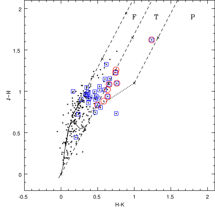
Figure 17.— (Left panel): The NIR TCD for the stars in the region of NGC 1931. (Right panel): Same as left panel but for the reference region. The continuous and thick dashed curves represent the unreddened MS and giant branch (Bessell & Brett, 1988), respectively. The dotted line indicates the locus of unreddened CTTSs (Meyer et al., 1997). The parallel dashed lines are the reddening vectors drawn from the tip (spectral type M4) of the giant branch (left reddening line), from the base (spectral type $A0$) of the MS branch (middle reddening line) and from the tip of the intrinsic CTTS line (right reddening line). The crosses on the reddening vectors show an increment of $A_{V}$ = 5 mag. The sources shown with circles are the NIR excess sources whereas the sources shown with square symbols are Class II sources identified on the basis of MIR data (cf. Sec 6.2.2).

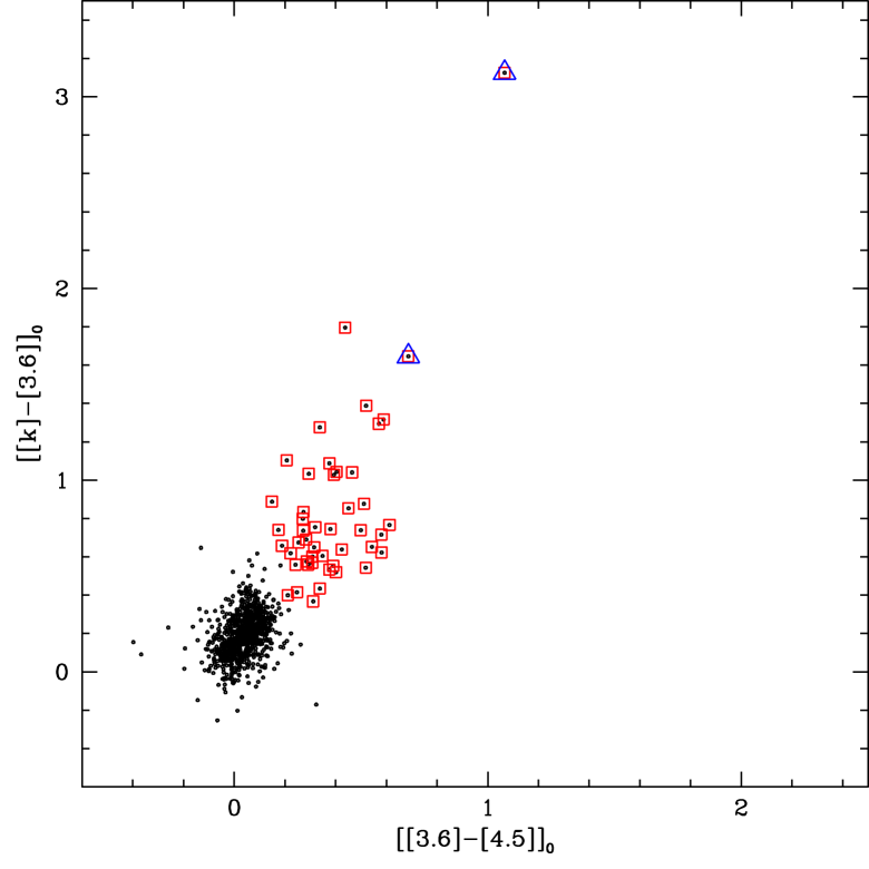
Figure 18.— $[[K]-[3.6]]_{0}$ versus $[[3.6]-[4.5]]_{0}$ TCD for the IRAC sources having 2MASS K-band counter parts. The triangle and squares represent Class I and Class II sources respectively.

The Spitzer MIR observations (3.6 $\mu$m and 4.5 $\mu$m) for the NGC 1931 region are also available. Since young stars in the NGC 1931 could be deeply embedded, the MIR observations can provide a deeper insight into the embedded YSOs. YSOs occupy distinct regions in the IRAC color plane according to their nature; this makes MIR TCDs a very useful tool for the classification of YSOs. Since 8.0 $\mu$m data are not available for the region, we used $[[K]-[3.6]]_{0}$ and $[[3.6]-[4.5]]_{0}$ TCD (cf. Gutermuth et al., 2009) to identify the deeply embedded YSOs. Fig. 18 presents a $[[K]-[3.6]]_{0}$ versus $[[3.6]-[4.5]]_{0}$ TCD for the observed sources. The identified Class I and Class II sources along with photometric data (optical: present work, $JHK_{s}$: 2MASS, 3.6 $\mu$m and 4.5 $\mu$m: Spitzer, 3.4 $\mu$m and 4.6 $\mu$m and 12 $\mu$m: WISE) are given in Tables 7 & 8. The 3.4 $\mu$m, 4.6 $\mu$m and 12 $\mu$m data have been taken from WISE database (http://irsa.ipac.caltech.edu/).

6.2.3 On the basis of optical & NIR CMDs and NIR TCD

Figure 19.— The $V/(V-I)$, $J/(J-H)$ CMDs and $(J-H)/(H-K)$ TCD for the stars having polarimetric observations but are not classified as probable members in Sec 5.2. The stars shown with star symbols are considered as probable members.The symbols are same as in Fig. 7.

Figure 19 shows $V/(V-I)$ and $J/(J-H)$ CMDs as well as $(J-H)/(H-K)$ two-color-diagram (TCD) for the remaining stars having polarimetric data but are not classified as probable members in Sec 5.2. We found a few stars located near 1 Myr isochrone in both the CMDs. These are shown by star symbols. Four stars #46, #58, #72 and #88 are located near the extension of T-Tauri stars (TTSs) locus by Meyer et al. (1997) in $(J-H)/(H-K)$ TCD. The disk accretion rates $\dot{M}_{disk}$ estimated using the spectral energy distribution (cf. Sec 6.4) for the stars #46 and #72 are of the order of $10^{-9}$ and $10^{-7}$ $M_{\sun}$/yr which are comparable to the Class II sources. We presume these could be weak line TTSs with small NIR excess. The star #139 could also be a reddened WTTs, whereas the star # 236 could be HAe/Be star. The star # 236 is identified as a Class II source on the basis of NIR and MIR data (cf. Sec 6.2.2). The $\dot{M}_{disk}$ for #236 and #139 is estimated to be $0.8\times 10^{-8}$ $M_{\sun}$/yr and $0.8\times 10^{-7}$ $M_{\sun}$/yr, respectively.

6.3. CMD for the PMS sources

Figure 20.— $V$ versus $(V-I)$ CMD for the identified YSOs (Class I, Class II and NIR-excess sources respectively shown with open triangles, squares and circles) identified on the basis of NIR (cf. Sec 6.2.1) and MIR (cf. Sec 6.2.2) data. The star symbols represent probable YSOs as identified in Sec 6.2.3. The PMS isochrones for 1, 2, 5 and 10 Myr by Siess, Dufour, & Forestini (2000) and isochrone for 1 Myr by Marigo et al. (2008) are drawn as dashed and continuous curves. All the isochrones are corrected for the cluster distance and reddening. The average error in $V$ and $(V-I)$ colors are shown in the right side of the figure.

The $V/(V-I)$ CMD for the YSOs identified in Sec 6.2 is shown in Fig. 20. PMS isochrones by Siess et al. (2000) for 1, 2, 5 and 10 Myr (dashed lines) and post-main sequence isochrone for 1 Myr by Marigo et al. (2008) (continuous curve) corrected for cluster distance (2.3 kpc) and minimum reddening ($E(B-V)$=0.5) are also shown. Figure 20 reveals that a majority of the sources have ages $\textless$ 5 Myr with a possible age spread of $\sim$5 Myr. Since the reddening vector in $V/(V-I)$ CMD is nearly parallel to the PMS isochrone, the presence of variable extinction in the region will not affect the age estimation significantly. The age and mass of each YSO have been estimated using the V/$(V-I)$ CMD, as discussed by  Pandey et al. (2008) and  Chauhan et al. (2009) and are given in Table 9. It is worthwhile to point out that the estimation of the ages and masses of the PMS stars by comparing their locations in the CMDs with the theoretical isochrones is prone to random as well as systematic errors  (see e.g. Hillenbrand, 2005; Hillenbrand et al., 2008; Chauhan et al., 2009, 2011b). The effect of random errors due to photometric errors and reddening estimation in determination of ages and masses has been estimated by propagating the random errors to their observed estimation by assuming normal error distribution and using the Monte-Carlo simulations (cf. Chauhan et al., 2009). The systematic errors could be due to the use of different PMS evolutionary models and the error in distance estimation etc. Since we are using evolutionary models by Siess et al. (2000) to estimate the age of all the YSOs in the region, we presume that the age estimation is affected only by the random errors. The presence of binaries may also introduce errors in the age determination. Binarity will brighten the star, consequently the CMD will yield a lower age estimate. In the case of an equal mass binary we expect an error of $\sim 50-60\%$ in the PMS age estimation. However, it is difficult to estimate the influence of binaries/variables on mean age estimation as the fraction of binaries/variables is not known. In the study of TTSs in the H ii region IC 1396, Barentsen et al. (2011) pointed out that the number of binaries in their sample of TTSs could be very low as close binaries loose their disk significantly faster than single stars (cf. Bouwman et al., 2006). Estimated ages and masses of the YSOs range from $\sim$ 0.1 to 5 Myr and $\sim 0.3-3.5M_{\sun}$ respectively, which are comparable with the lifetime and masses of TTSs. The age spread indicates a non-coeval star formation in this region.

6.4. Physical state of the YSOs

To characterize the circumstellar disk properties of YSOs, we analyzed the spectral energy distributions (SEDs) using the fitting tool of Robitaille et al. (2007). The SED fitting tool fits thousands of models to the observed SED simultaneously. This SED fitting tool determines their physical parameters like mass (M_⋆), age, interstellar extinction ($A_{V}$), temperature ($T_{\star}$), disk mass, disk mass accretion rate ($\dot{M}_{acc}$), etc. The SED fitting tool fits each of the models to the data, allowing both the distance and foreground extinction to be free parameters. Since we do not have spectral type information for the identified YSOs, we estimated $A_{V}$ by tracing back sources along the reddening vector to the intrinsic locus of TTS (Meyer et al., 1997) in $(J-H)/(H-K)$ TCD. Thus estimated value of $A_{V}$ is considered as the maximum $A_{V}$ whereas the foreground extinction for the YSOs, towards NGC 1931 is considered as the minimum $A_{V}$. The distance range is adopted as 2.1 to 2.5 kpc. The error in NIR and MIR flux estimates due to possible uncertainties in the calibration, extinction, and intrinsic object variability was set as 10$-$20%. Figure 21 shows an example of SED of the resulting model for a Class II source #236. We obtained physical parameters for all the sources adopting an approach similar to that of Robitaille et al. (2007) by considering those models that satisfy $\chi^{2}$-$\chi^{2}_{min}\textless$ $2N_{data}$, where $\chi^{2}_{min}$ is the goodness-of-fit parameter for the best-fit model and $N_{data}$ is the number of observational input data points. The relevant parameters are obtained from the weighted mean and the standard deviation of these models, weighted by e${}^{({{-\chi}^{2}}/2)}$ of each model and are shown in Table 10, which reveals that majority of the Class II sources have disk accretion rate of the order of $\sim$ $10^{-7}-10^{-8}$ $M_{\sun}$ yr^-1. The parameters support the classification of YSOs obtained on the basis of CMDs and NIR/MIR TCDs. We would like to mention that the stellar ages given in Table 10 are only approximate and in the absence of far-infrared (FIR) to millimeter data the disk parameters, should be taken with a caution, however these parameters can still be used as a quantitative indicator of stellar youth.

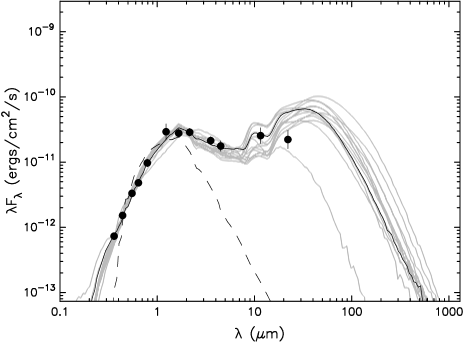
Figure 21.— The SED for a Class II source #236. The black line shows the best fit, and the gray lines show subsequent good fits with $\chi^{2}$-$\chi^{2}_{min}\textless$ $2N_{data}$. The dashed line shows the stellar photosphere corresponding to the central source of the best fitting model. The filled circles denote the input flux values using the data given in Tables 7 & 8.

7. INITIAL MASS FUNCTION AND K-BAND LUMINOSITY FUNCTION

The distribution of stellar masses for a star formation event in a given volume of space is known as initial mass function (IMF) and in combination with star formation rate, the IMF dictates the evolution and fate of galaxies and star clusters (Kroupa, 2002). The MF of young clusters can be considered as the IMF as they are too young to lose significant number of members either by dynamical or by stellar evolution.

The MF is often expressed by a power law, $N(\log m)\propto m^{\Gamma}$ and the slope of the MF is given as: $\Gamma=d\log N(\log m)/d\log m$ where $N(\log m)$ is the number of stars per unit logarithmic mass interval. For the mass range 0.4 $\textless$ $M/M_{\odot}$ $\leqslant 10$, the classical value derived by Salpeter (1955) for the slope of MF is $\Gamma=-1.35$.

Figure 22.— The MF for the whole cluster region (upper panel), the northern (middle panel) and southern (bottom panel) regions. The continuous line is the fit to the data excluding the points shown by open circles, whereas the dashed line shows fit for the entire sample.

With the help of the statistically cleaned CMD, shown in Fig. 16, we can derive the MF using the theoretical evolutionary models. Since the age of the massive cluster members could be $\sim$ 5 Myr, the stars having V $\leqslant$ 15 mag ($V_{0}$ $\leqslant$ 13.5 mag; M $\geqslant$ $2M_{\odot}$) are considered as MS stars. For these stars, the LF was converted to a MF using the theoretical models by Marigo et al. (2008) (cf. Pandey et al., 2001, 2005). The MF for the PMS stars have been obtained by counting the number of stars having age $\leqslant$ 5 Myr in various mass bins shown as evolutionary tracks in Fig. 16. The resulting MF for the whole cluster region, the northern and southern regions (cf. Fig. 3) is plotted in Fig. 22. The slope ($\Gamma$) of the MF in the mass range 0.5 $\textless$ $M/M_{\odot}$ $\textless$ 9.5 for the northern, southern clusters and for the combined region comes out to be $-0.92\pm 0.21$, $-0.87\pm 0.15$ and $-0.90\pm 0.16$ respectively, which seems to be shallower than the Salpeter (1955) value (-1.35). However, a careful look of the MF in the northern cluster reveals a break in the power law at $\sim$ 0.8$-$1.0 $M_{\odot}$. Excluding the points shown by open cirlces, the slope of the MF in the range 0.8 $\textless$ $M/M_{\odot}$ $\textless$ 9.8 is found to be -1.26$\pm$0.23, -0.98$\pm$0.22 and -1.15$\pm$0.19 for the northern, southern and for the whole cluster regions, respectively. The break in the MF slope has also been reported in the case of two clusters, namely Stock 8 and NGC 1893 located near the NGC 1931. In the case of young clusters, Stock 8 (Jose et al., 2008) and NGC 1893 (Sharma et al., 2007), the break was reported at $\sim$$1-2$$M_{\odot}$.

Figure 23.— Comparison of the observed KLF (filled circles) and the simulated KLF (triangles) from the Galactic model (see text). The error bars represent $\pm\sqrt{N}$ errors.

During the last decade several studies have focused on determination of the $K$-band luminosity function (KLF) of young open clusters (e.g Lada & Lada, 2003; Ojha et al., 2004; Sharma et al., 2007; Sanchawala et al., 2007; Pandey et al., 2008; Jose et al., 2008, 2011). The KLF is being used to investigate the IMF and star formation of young embedded clusters. In order to obtain the KLF in the region, we have assumed that the NIR data is 99% complete up to $\sim$ 15.7, 15.1 and 14.3 mag in $J$, $H$ and $K_{s}$ bands, respectively as mentioned in Sec 3.1. The Besançon Galactic model of stellar population synthesis (Robin et al., 2003) was used to estimate the foreground/background field star contamination in the present sample. The star counts both towards the cluster region and towards the direction of the reference field we estimated and checked the validity of the simulated model by comparing the model KLF with that of the reference field and found that the two KLFs match rather well (Fig. 23). The advantage of this method is that we can separate the foreground ($d~{}\textless~{}2.3$ kpc) and the background ($d~{}\textgreater~{}2.3$ kpc) field star contamination. The foreground extinction towards the cluster region is found to be $A_{V}\sim$ 1.6 mag. The model simulations with $d~{}\textless~{}2.3$ kpc and $A_{V}$ = 1.6 mag give the foreground contamination, and that with $d~{}\textgreater~{}2.3$ kpc and $A_{V}$ = 2.8 mag give the background population. We thus determined the fraction of the contaminating stars (foreground+background) over the total model counts. This fraction was used to scale the nearby reference region and subsequently the modified star counts of the reference region were subtracted from the KLF of the cluster to obtain the final corrected KLF. This KLF is expressed by the following power-law:

${{\rm{d}N(K)}\over{\rm{d}K}}\propto 10^{\alpha K}$

where ${\rm{d}N(K)}\over{\rm{d}K}$ is the number of stars per 0.5 magnitude bin and $\alpha$ is the slope of the power law. Fig. 24 shows the KLF for the cluster region which yields a slope of $\alpha$ = 0.38$\pm$0.13, 0.29$\pm$0.06 and 0.36$\pm$0.08 for the northern, southern regions and for the whole cluster region, respectively. The slopes in the northern and southern regions within the error are rather same and similar to the average slopes ($\alpha\sim 0.4$) for young clusters  (Lada & Lada, 1991, 1995, 2003) but higher than the values (0.27$-$0.31) obtained for Be 59 (Pandey et al., 2008), Stock 8 (Jose et al., 2008) and NGC 2175 region (Jose et al., 2012).

Figure 24.— The corrected KLF for North, South and whole cluster regions. The straight line is the least-square fit to the data. The error bars represent $\pm\sqrt{N}$ errors.

8. Star formation scenario in the NGC 1931 region

The massive stars in star-forming regions have strong influence and can significantly affect the entire region. The star formation in the region may be terminated as energetic stellar winds from massive stars can evaporate nearby clouds. Alternatively, stellar winds and shock waves from a supernova explosion may squeeze molecular clouds and induce next generation of star formation. Elmegreen & Lada (1977) propose that the expanding ionization fronts from the massive star(s) play a constructive role in inciting a sequence of star formation activities in the neighborhood. The distribution of YSOs and the morphological details of the environment around NGC 1931 can be used to probe the star formation scenario in the region.

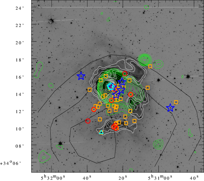
Figure 25.— Spatial distribution of Class II sources (square symbols), Class I sources (triangles), NIR excess sources (circles) and probable PMS sources (open star symbols) overlaid on K-band image. The open pentagon symbols denote two ionizing stars #7 and #11. The black continuous contours represent ¹²CO emission from Leisawitz et al. (1989). The NVSS 1.4 GHz radio emission contours (thin green contours) and MSX A-band intensity contours (thick white contours) have also been shown. The minimum and maximum levels of NVSS contours are 0.001 Jy/beam and 0.187 Jy/beam respectively, whereas the minimum and maximum levels of MSX A-band contours are 2.01$\times$10^-6 w/m²-Sr and 2.64$\times$10^-5 w/m²-Sr respectively. North is up and east is to the left. Abscissa and ordinate show the RA (J2000) and Dec (J2000), respectively. Color version of the figure is available in online journal.

In Fig. 25, the $NRAO$ VLA Sky Survey (NVSS) 1.4 GHz radio continuum emission contours (thin green contours) and MSX $A$-band (8.3 $\mu$m) MIR contours (thick white contours) along with distribution of YSOs are overlaid on the IRAC 3.4 $\mu$m image. In literature we could not find any detailed observations to probe the molecular cloud associated with NGC 1931. The only available is the ¹²CO contour map of Sh2-237 region traced from figure 27(c) of Leisawitz, Bash, & Thaddeus (1989), which is also shown in Fig. 25 as black contours. Although the resolution is poor, a moderate-sized molecular cloud (NGC 1931C; Leisawitz, Bash, & Thaddeus, 1989) of $\sim 6.9\times 10^{3}M_{\odot}$ is found to be associated with the cluster. The peak of the ¹²CO contours is located at the south-east of the cluster center, with a peak value of $H_{2}$ column density $N(H_{2})$ of $\sim 3\times 10^{21}cm^{-2}$.

The morphology of the radio continuum emission contours reveals that the eastern region is an ionization-bounded zone, whereas the decreasing intensity distribution towards the south-west direction suggests that this region could be density bounded. There seems to be a flow of ionized gas in the south-west direction, as expected in case of Champagne flow model (Tenorio-Tagle, 1979).

Sh2-237 is rather a spherical H ii region around ionizing star(s) and is nearly surrounded by a dust ring, as revealed by MIR emission in the MSX A-band (centered at 8.3 $\mu$m) as well as in the Spitzer IRAC channel 2 (centered at 4.5 $\mu$m). The far-ultraviolet (UV) radiation can escape from the H ii region and penetrate the surface of molecular clouds leading to the formation of photo-dissociation region (PDR) in the surface layer of the clouds. Polycyclic aromatic hydrocarbons (PAHs) within the PDR are excited by the UV photons re-emitting their energy at MIR wavelengths, particularly between 6 and 10 $\mu$m. The A-band (8.3 $\mu$m) of MSX includes several discrete PAH emission features (e.g., 6.6, 7.7, and 8.6 $\mu$m) in addition to the contribution from the thermal continuum component from hot dust. The ring of PAH emission lies beyond the ionization front (IF), indicating the interface between the ionized and molecular gas (i.e. PDR). The absence of 8 $\mu$m emission in the interior of the H ii region is interpreted as the destruction of PAH molecules by intense UV radiation of the ionizing star.

The 1.4 GHz radio continuum emission contours derived from the NVSS (Condon et al., 1998) reveal a peak around $\alpha_{2000}\sim 05^{h}31^{m}28^{s}$ and $\delta_{2000}\sim+34\arcdeg 14\arcmin 48\arcsec$. The integrated flux density of the radio continuum above $3\sigma$ level is estimated to be 0.76 Jy. Leisawitz et al. (1989) have reported the flux density of the H ii region as 0.6 Jy. We estimated the number of Lyman continuum photons ($N_{Lyc}$) emitted per second, and hence the spectral type of the exciting star using the flux density of 0.76 Jy together with the assumed distance and by assuming a spherical symmetry for the ionized region and neglecting absorption of UV radiation by dust inside the H ii region. Assuming a typical electron temperature in region as 8000 K (see e.g., Samal et al., 2007), the relation given by Martín-Hernández, van der Hulst, & Tielens (2003) yields log $N_{Lyc}$ = 47.26, which corresponds to a MS spectral type of $\sim$B0.5 (Panagia, 1973; Schaerer & de Koter, 1997). The region has two brightest stars (cf. Fig. 14; #7, $M_{V}$ $\sim$ -2.24 and #11, $M_{V}$ $\sim$ -2.03; spectral type $\sim$ B2) associated with the northern nebulosity. If these stars are the ionization sources of the region, the $N_{Lyc}$ produced by these stars will be $log(N_{Lyc})\approx 45.0$. The $N_{Lyc}$ derived from 1.4 GHz radio observations are quite high relative to the available stellar content estimated from the broad-band photometry.

The spectral type of the two brightest stars (probable ionizing stars) is found to be $\sim$ B2V. The stars seem to be on the MS. The MS life-time of B2 type star is $\sim$25 Myr (Leinert, 2006). This suggests that the H ii region may still be under expansion. The dynamical age of Sh2-237 can be estimated using the model by Dyson & Williams (1997) with an assumption that the ionized gas of pure hydrogen is at a constant temperature in an uniform medium of constant density. If the H ii region associated with Sh2-237 has $N_{Lyc}$ $\sim 1.855\times 10^{47}$ (log$N_{Lyc}$ $\sim$ 47.26) effective ionizing photons per second and is expanding into a homogeneous medium of typical density $10^{4}(10^{3})~{}{cm}^{-3}$, it will form a Str$\ddot{o}$mgren radius ($r_{s}$) of $\sim$ 0.022(0.10) pc. The initial phase is overpressured compared to the neutral gas and will expand into the medium of radius $r_{i}$ at time $t$ as

$$r_{i}=r_{s}\left(1+\frac{7~{}C_{II}~{}t}{4~{}r_{s}}\right)^{4/7}$$

The observed radius of the ionized gas from NVSS radio contours is found to be $\sim 2\farcm 4$ (cf. Fig. 25), which corresponds to a physical radius of about 1.6 pc at a distance of 2.3 kpc. In the literature the expansion velocity of the ionized front is reported as $\sim$ 4 km s^-1  (e.g., Moreno-Corral et al., 1993; Kang et al., 2009; Pomarès et al., 2009). Assuming an expansion speed ($C_{II}$) of 4 km s^-1 and typical density of the ionized gas as $10^{4}(10^{3})~{}cm^{-3}$, the dynamical age of the ionized region comes out to be $\sim$ 6 (2) Myr. The estimated dynamical age must be considered highly uncertain because of the assumption of an uniform medium, assumed velocity of expansion etc. Since the H ii region is found to be partially surrounded by the MSX dust emission, we would expect an expanding IF to be preceded by a swept-up shell of cool neutral gas as it erodes into a neutral cloud.

Fig. 25 also shows the distribution of identified YSOs. The distribution of YSOs does not seem to follow the stellar density distribution of the cluster region and hence we presume that these YSOs could be next generation stars. A significant number of YSOs are found to be associated with the dust ring as revealed by MIR emission in the MSX A-band (cf. Fig. 25). This could be an indication of triggered star formation. In the literature two mechanisms which could be responsible for triggered star formation have been discussed. These are “radiation-driven implosion” (RDI) and “collect-and-collapse” models.

Detailed model calculations of the RDI process have been carried out by several authors  (e.g., Bertoldi, 1989; Lefloch & Lazareff, 1995; Lefloch et al., 1997; De Vries et al., 2002; Kessel-Deynet & Burkert, 2003; Miao et al., 2006). In this process, a pre-existing dense clump is exposed to the ionizing radiation from massive stars of the previous generation. The head part of the clump collapses due to the high pressure of the ionized gas and the self-gravity, which consequently leads to the formation of next generation stars. The signature of the $RDI$ process is the anisotropic density distribution in a relatively small molecular cloud surrounded by a curved ionization/shock front (bright rim) as well as a group of YSOs aligned from the bright rim to the direction of the ionizing source.

In the “collect and collapse” process, which was proposed by  Elmegreen & Lada (1977), as the H ii region expands, the surrounding neutral material is collected between the ionization front and the shock front which precedes the former. With time the layer gets massive and consequently becomes gravitationally unstable and collapses to form stars of the second generation including massive stars. Recent simulations of this process are shown by Hosokawa & Inutsuka (2005, 2006) and Dale et al. (2007). An observational signature of the process is the presence of a dense layer and massive condensations adjacent to an H ii region (e.g., Deharveng et al., 2003).

The YSOs do not show any aligned distribution as expected in the case of RDI and hence the RDI cannot be the process for triggering of the next generation of stars. Since the probable ionization sources in the region have spectral types of $\sim$B2, the maximum MS life time of a B2 type star could be $\sim$25 Myr (cf. Leinert, 2006). The dynamical age of the ionized region is estimated in the range of $\sim$2-6 Myr. The spherical morphology of the ionized region partially surrounded by MSX dust emission in the mid-IR (see Fig. 25) and association of YSOs (having mean age $\sim$ 2$\pm$1 Myr) with the dust region indicate triggered star formation which could be due to “collect-and-collapse” process. Some of the YSOs are not found to be associated with the dust and are distributed in the central part. We presume that these sources may be located in the collected material lying in the outer skin of the molecular cloud towards the line of sight of the observer. The ¹²CO map by Leisawitz et al. (1989) also suggests that the cluster is located at the extreme end of the molecular cloud. The overall star formation scenario in the NGC 1931 region also seems to indicate for a blister model of star formation as suggested by Zuckerman (1973). Israel (1978) has also found that the majority of H ii regions were located at the edges of molecular clouds and have structure suggestive of IF surrounded by less dense envelopes.

However, in a recent model calculation, Walch et al. (2011) argued that the clumps around the edge of H ii regions do not require the collect and collapse process and can be explained by the pre-existing non-uniform density distribution of the molecular cloud into which the H ii region expands. This star formation scenario can also be speculated for the NGC 1931 region.

9. Conclusions

In this study we report photometric and polarimetric observations towards the direction of the NGC 1931 cluster region. The aim of this study was to investigate the properties of dust grains in the ISM towards the direction of the clusters as well as the properties of intracluster dust and star formation scenario in the region. The following are the main conclusions of this study:

• We have shown that the polarization measurements in combination with the $(U-B)-(B-V)$ color-color diagram provide a better identification of the cluster members.

• The distance to the cluster is estimated using the probable members identified on the basis of polarimetric and photometric data. The estimated distance of 2.3$\pm$0.3 kpc is in agreement with the values obtained by us in previous studies. The interstellar extinction in the cluster region is found to be variable with $E(B-V)_{min}~{}\simeq~{}0.5$ mag, $E(B-V)_{max}~{}\simeq~{}0.9$ mag. Both, the polarimetric as well as photometric studies indicate that the ratio of total-to-selective extinction in the cluster region, $R_{cluster}$, could be higher than the average.

• The estimated mean values of $P_{V}$ and $\theta_{V}$ for the cluster NGC 1931 are found to be similar to those of Stock 8 which is located approximately at similar distance of the cluster NGC 1931.

• The weighted mean of the $P_{max}$ and $\lambda_{max}$ values for NGC 1931 are found to be 2.51$\pm$0.03 per cent and 0.57$\pm$0.01 $\mu$m, respectively. The estimated $\lambda_{max}$ is slightly higher than that for the diffuse ISM which indicates that the average size of the dust grains within the cluster NGC 1931 may be slightly larger than that of the diffuse ISM.

• The polarization efficiency of the dust grains towards NGC 1931 is found to be less than that of the diffuse ISM. This could be due to the average extinction law in the foreground medium and a differing reddening law in the intra-cluster medium.

• The stellar density distribution in the region reveals two separate clustering in the region. The reddening in the northern regions is found to be variable. The radial extent of the region is estimated to be $\sim$3.5 arcmin.

• The statistically cleaned CMD indicates a PMS population in the region having ages $\sim$ 1$-$5 Myr.

• The slope of the mass function (-0.98$\pm$0.22) in the southern region in the mass range 0.8 $\textless$ $M/M_{\sun}$ $\textless$ 9.8 is found to be shallower in comparison to that in the northern region (-1.26$\pm$0.23), which is comparable to the Salpeter value (-1.35). The KLF of the region is found to be comparable to the average value of slope ($\sim$ 0.4; cf. Lada & Lada, 2003) for young clusters. However, the slope of the KLF is steeper in the northern region which indicates relatively fainter stars in the northern region as compared to the southern region.

• The region is probably ionized by two B2 MS type stars (#7 and #11). However, the $N_{Lyc}$ derived from 1.4 GHz radio observations are quite high relative to the available stellar content estimated from the broad-band photometry. The maximum MS age of B2 stars could be $\sim$25 Myr. The YSOs identified on the basis of NIR/MIR data have masses $\sim$1-3.5$M_{\odot}$. The mean age of the YSOs in the region is found to be 2$\pm$1 Myr which suggests that the YSOs must be younger than the ionizing sources of the region. The morphology of the region and ages of the YSOs and ionization sources indicate triggered star formation in the region.

Table 6Observed polarzation, polarization angles and estimated Serkowski parameters.

Star ID	R.A (J2000)	DEC (J2000)	$P_{V}\pm\epsilon$	$\theta_{V}\pm\epsilon$	$P_{Rc}\pm\epsilon$	$\theta_{Rc}\pm\epsilon$	$P_{Ic}\pm\epsilon$	$\theta_{Ic}\pm\epsilon$	$P_{max}\pm\epsilon$	$\lambda_{max}\pm\epsilon$	$\sigma_{1}$	$\overline{\epsilon}$
	(h m s)	($\arcdeg~{}\arcmin~{}\arcsec$)	(per cent)	($\arcdeg$)	(per cent)	($\arcdeg$)	(per cent)	($\arcdeg$)	(percent)	($\mu$m)
(1)	(2)	(3)	(4)	(5)	(6)	(7)	(8)	(9)	(10)	(11)	(12)	(13)
Stars with $V(RI)_{c}$ passband data
3	5 31 26.304	34 11 9.838	2.11 $\pm$ 0.09	153.1 $\pm$ 1.1	2.25 $\pm$ 0.08	151.7 $\pm$ 0.9	1.83 $\pm$ 0.09	150.3 $\pm$ 1.4	2.19 $\pm$ 0.06	0.58 $\pm$ 0.04	1.98	1.22
5	5 31 40.241	34 14 26.232	2.29 $\pm$ 0.10	156.3 $\pm$ 1.1	2.39 $\pm$ 0.08	156.1 $\pm$ 1.0	2.16 $\pm$ 0.09	156.2 $\pm$ 1.1	2.37 $\pm$ 0.06	0.61 $\pm$ 0.04	0.61	0.10
8	5 31 9.989	34 11 13.049	0.38 $\pm$ 0.11	6.1 $\pm$ 6.4	0.41 $\pm$ 0.09	2.7 $\pm$ 5.2	0.33 $\pm$ 0.11	0.3 $\pm$ 7.3	0.40 $\pm$ 0.08	0.57 $\pm$ 0.25	0.34	0.50
9	5 31 21.278	34 11 17.927	2.82 $\pm$ 0.12	155.6 $\pm$ 1.2	2.71 $\pm$ 0.11	155.8 $\pm$ 1.2	2.57 $\pm$ 0.14	156.7 $\pm$ 1.4	2.82 $\pm$ 0.09	0.58 $\pm$ 0.04	0.67	0.37
10	5 31 43.544	34 16 30.803	0.65 $\pm$ 0.16	172.0 $\pm$ 5.8	0.35 $\pm$ 0.14	163.0 $\pm$ 8.8	0.66 $\pm$ 0.13	4.7 $\pm$ 5.0	–	–	–	–
12	5 31 20.102	34 13 40.692	2.91 $\pm$ 0.16	154.3 $\pm$ 1.5	2.78 $\pm$ 0.14	151.7 $\pm$ 1.4	2.38 $\pm$ 0.17	156.1 $\pm$ 1.9	2.93 $\pm$ 0.15	0.53 $\pm$ 0.05	0.32	0.91
13	5 31 16.265	34 11 51.515	1.95 $\pm$ 0.20	151.9 $\pm$ 2.9	1.84 $\pm$ 0.18	151.6 $\pm$ 2.6	2.18 $\pm$ 0.21	159.7 $\pm$ 2.6	2.05 $\pm$ 0.13	0.73 $\pm$ 0.12	1.43	1.00
15	5 31 27.834	34 18 13.799	2.19 $\pm$ 0.25	160.5 $\pm$ 3.0	2.57 $\pm$ 0.22	148.3 $\pm$ 2.4	1.79 $\pm$ 0.24	141.4 $\pm$ 3.7	2.36 $\pm$ 0.20	0.56 $\pm$ 0.09	1.81	3.43
16	5 31 0.899	34 11 39.829	2.07 $\pm$ 0.24	158.2 $\pm$ 3.2	2.30 $\pm$ 0.17	152.3 $\pm$ 2.0	2.07 $\pm$ 0.16	152.6 $\pm$ 2.1	2.23 $\pm$ 0.12	0.64 $\pm$ 0.09	0.60	1.58
20	5 31 6.557	34 8 44.956	2.29 $\pm$ 0.25	151.8 $\pm$ 3.1	2.18 $\pm$ 0.17	151.1 $\pm$ 2.2	1.85 $\pm$ 0.17	149.6 $\pm$ 2.5	2.31 $\pm$ 0.24	0.52 $\pm$ 0.08	0.20	0.38
21	5 31 11.433	34 12 42.754	1.85 $\pm$ 0.25	154.6 $\pm$ 3.8	2.08 $\pm$ 0.23	154.7 $\pm$ 3.0	1.30 $\pm$ 0.28	153.9 $\pm$ 5.7	1.98 $\pm$ 0.27	0.51 $\pm$ 0.11	1.59	0.06
22	5 31 25.078	34 11 36.672	1.52 $\pm$ 0.24	166.6 $\pm$ 4.3	2.20 $\pm$ 0.21	161.1 $\pm$ 2.6	1.12 $\pm$ 0.24	160.5 $\pm$ 5.6	1.79 $\pm$ 0.19	0.56 $\pm$ 0.12	3.13	0.94
23	5 31 44.304	34 12 2.462	1.80 $\pm$ 0.30	159.5 $\pm$ 4.4	2.03 $\pm$ 0.21	164.7 $\pm$ 2.8	1.82 $\pm$ 0.18	168.5 $\pm$ 2.7	1.96 $\pm$ 0.15	0.64 $\pm$ 0.12	0.46	1.45
26	5 31 24.496	34 9 52.686	2.32 $\pm$ 0.29	163.7 $\pm$ 3.4	1.89 $\pm$ 0.21	156.4 $\pm$ 3.0	2.25 $\pm$ 0.23	168.1 $\pm$ 2.7	2.18 $\pm$ 0.15	0.64 $\pm$ 0.12	1.81	1.27
30	5 31 40.680	34 13 48.137	1.80 $\pm$ 0.36	159.8 $\pm$ 5.3	2.03 $\pm$ 0.30	165.3 $\pm$ 4.0	1.90 $\pm$ 0.30	163.3 $\pm$ 4.4	1.98 $\pm$ 0.19	0.69 $\pm$ 0.18	0.20	0.67
32	5 31 18.638	34 11 17.844	2.64 $\pm$ 0.30	155.5 $\pm$ 3.1	1.86 $\pm$ 0.24	148.4 $\pm$ 3.5	1.82 $\pm$ 0.26	154.0 $\pm$ 3.8	2.70 $\pm$ 0.56	0.42 $\pm$ 0.08	1.18	0.83
37	5 30 54.507	34 10 49.141	3.50 $\pm$ 0.33	150.9 $\pm$ 2.6	2.90 $\pm$ 0.23	148.6 $\pm$ 2.2	2.58 $\pm$ 0.21	152.6 $\pm$ 2.3	3.47 $\pm$ 0.41	0.47 $\pm$ 0.06	0.61	0.56
41	5 31 45.626	34 13 31.739	3.32 $\pm$ 0.44	166.4 $\pm$ 3.5	2.62 $\pm$ 0.25	163.4 $\pm$ 2.6	2.68 $\pm$ 0.17	164.0 $\pm$ 1.8	2.99 $\pm$ 0.31	0.56 $\pm$ 0.09	1.41	0.67
45	5 31 7.708	34 14 16.768	2.53 $\pm$ 0.40	153.5 $\pm$ 4.4	2.13 $\pm$ 0.33	146.2 $\pm$ 4.2	1.45 $\pm$ 0.37	153.9 $\pm$ 6.8	2.94 $\pm$ 1.00	0.38 $\pm$ 0.11	0.43	0.50
46	5 31 43.463	34 15 59.080	2.10 $\pm$ 0.44	149.6 $\pm$ 5.7	2.44 $\pm$ 0.31	158.9 $\pm$ 3.4	1.94 $\pm$ 0.27	151.8 $\pm$ 3.9	2.30 $\pm$ 0.30	0.58 $\pm$ 0.14	0.84	0.88
47	5 30 53.075	34 11 45.953	2.28 $\pm$ 0.40	149.2 $\pm$ 4.8	2.49 $\pm$ 0.34	155.9 $\pm$ 3.8	2.63 $\pm$ 0.40	159.1 $\pm$ 4.2	2.59 $\pm$ 0.29	0.76 $\pm$ 0.19	0.23	1.30
48	5 31 46.759	34 14 11.717	2.44 $\pm$ 0.45	145.7 $\pm$ 5.1	2.19 $\pm$ 0.30	160.6 $\pm$ 3.8	1.57 $\pm$ 0.25	148.1 $\pm$ 4.3	2.73 $\pm$ 0.80	0.41 $\pm$ 0.10	0.52	1.31
51	5 31 20.036	34 10 7.406	2.16 $\pm$ 0.41	149.5 $\pm$ 5.1	1.77 $\pm$ 0.35	152.0 $\pm$ 5.4	1.49 $\pm$ 0.42	165.8 $\pm$ 7.6	2.25 $\pm$ 0.71	0.43 $\pm$ 0.15	0.14	1.04
52	5 30 59.940	34 12 44.003	1.17 $\pm$ 0.44	158.3 $\pm$ 10.1	1.52 $\pm$ 0.35	157.7 $\pm$ 6.3	2.44 $\pm$ 0.39	163.9 $\pm$ 4.4	–	–
53	5 30 59.192	34 8 31.110	2.34 $\pm$ 0.43	152.3 $\pm$ 5.0	1.72 $\pm$ 0.35	143.3 $\pm$ 5.5	1.94 $\pm$ 0.40	153.8 $\pm$ 5.5	2.19 $\pm$ 0.47	0.50 $\pm$ 0.16	1.04	0.65
55	5 30 59.360	34 14 20.011	2.25 $\pm$ 0.47	155.5 $\pm$ 5.7	2.45 $\pm$ 0.41	158.8 $\pm$ 4.7	2.21 $\pm$ 0.49	158.3 $\pm$ 6.1	2.39 $\pm$ 0.27	0.64 $\pm$ 0.20	0.21	0.37
57	5 31 20.978	34 13 47.093	3.18 $\pm$ 0.43	155.7 $\pm$ 3.8	2.47 $\pm$ 0.34	152.9 $\pm$ 3.8	2.51 $\pm$ 0.37	141.6 $\pm$ 4.1	3.04 $\pm$ 0.51	0.49 $\pm$ 0.11	0.97	1.44
58	5 30 53.382	34 12 17.334	2.67 $\pm$ 0.47	155.0 $\pm$ 4.9	2.52 $\pm$ 0.33	151.7 $\pm$ 3.6	2.47 $\pm$ 0.31	149.1 $\pm$ 3.4	2.64 $\pm$ 0.27	0.61 $\pm$ 0.14	0.37	0.77
71	5 31 1.710	34 8 26.826	2.88 $\pm$ 0.60	156.6 $\pm$ 5.8	2.13 $\pm$ 0.47	155.1 $\pm$ 6.0	2.60 $\pm$ 0.56	-3.3 $\pm$ 5.9	2.63 $\pm$ 0.48	0.56 $\pm$ 0.20	1.12	9.12
73	5 31 37.341	34 16 48.904	2.28 $\pm$ 0.64	153.5 $\pm$ 7.6	2.49 $\pm$ 0.52	159.6 $\pm$ 5.7	2.32 $\pm$ 0.50	162.3 $\pm$ 5.9	2.45 $\pm$ 0.33	0.66 $\pm$ 0.24	0.11	0.78
79	5 31 3.560	34 15 20.297	4.76 $\pm$ 0.55	151.8 $\pm$ 3.3	5.05 $\pm$ 0.47	135.2 $\pm$ 2.6	4.81 $\pm$ 0.53	167.0 $\pm$ 3.1	5.04 $\pm$ 0.31	0.66 $\pm$ 0.11	0.05	3.53
84	5 31 17.663	34 13 27.548	2.30 $\pm$ 0.57	157.1 $\pm$ 6.8	2.89 $\pm$ 0.48	158.1 $\pm$ 4.6	1.79 $\pm$ 0.57	148.9 $\pm$ 8.7	2.56 $\pm$ 0.47	0.55 $\pm$ 0.20	1.23	0.46
92	5 31 20.749	34 11 53.851	1.98 $\pm$ 0.61	167.9 $\pm$ 8.5	2.45 $\pm$ 0.47	156.0 $\pm$ 5.2	1.55 $\pm$ 0.49	136.9 $\pm$ 8.6	2.23 $\pm$ 0.58	0.53 $\pm$ 0.21	1.04	1.92
93	5 31 37.064	34 14 15.670	2.28 $\pm$ 0.69	146.6 $\pm$ 8.4	4.05 $\pm$ 0.58	158.8 $\pm$ 4.0	3.02 $\pm$ 0.56	160.9 $\pm$ 5.1	3.40 $\pm$ 0.50	0.79 $\pm$ 0.25	1.65	1.51
103	5 31 13.736	34 13 26.782	3.14 $\pm$ 0.70	154.0 $\pm$ 6.2	3.36 $\pm$ 0.57	147.1 $\pm$ 4.7	2.08 $\pm$ 0.66	142.9 $\pm$ 8.5	3.43 $\pm$ 0.97	0.47 $\pm$ 0.16	0.97	0.93
Stars embedded in the nebulosity
7	5 31 27.071	34 14 49.520	0.82 $\pm$ 0.11	148.9 $\pm$ 3.3	0.73 $\pm$ 0.09	131.8 $\pm$ 3.1	0.55 $\pm$ 0.09	99.4 $\pm$ 3.9	0.88 $\pm$ 0.18	0.43 $\pm$ 0.09	0.36	6.47
11	5 31 26.523	34 14 45.071	0.62 $\pm$ 0.13	162.9 $\pm$ 5.0	0.86 $\pm$ 0.10	170.6 $\pm$ 2.9	0.87 $\pm$ 0.10	26.7 $\pm$ 2.8	0.90 $\pm$ 0.13	0.89 $\pm$ 0.20	0.56	13.42
14	5 31 26.434	34 14 56.224	2.11 $\pm$ 0.22	140.4 $\pm$ 2.9	2.10 $\pm$ 0.12	143.6 $\pm$ 1.5	1.30 $\pm$ 0.19	127.8 $\pm$ 3.9	2.40 $\pm$ 0.36	0.44 $\pm$ 0.07	2.18	1.89
34	5 31 27.504	34 15 3.132	2.11 $\pm$ 0.37	156.0 $\pm$ 4.6	1.11 $\pm$ 0.29	135.0 $\pm$ 7.0	1.04 $\pm$ 0.29	175.0 $\pm$ 7.4	–	–	–	–
35	5 31 25.024	34 14 40.484	6.51 $\pm$ 0.32	159.1 $\pm$ 1.3	6.23 $\pm$ 0.23	163.3 $\pm$ 1.1	6.82 $\pm$ 0.20	163.4 $\pm$ 0.8	6.73 $\pm$ 0.14	0.71 $\pm$ 0.04	2.59	2.64
49	5 31 25.012	34 14 17.387	1.61 $\pm$ 0.49	158.2 $\pm$ 8.0	1.58 $\pm$ 0.40	135.6 $\pm$ 7.0	1.73 $\pm$ 0.41	130.0 $\pm$ 6.4	1.69 $\pm$ 0.27	0.71 $\pm$ 0.30	0.35	2.39
68	5 31 31.881	34 13 57.500	2.03 $\pm$ 0.57	152.1 $\pm$ 7.6	1.70 $\pm$ 0.42	149.6 $\pm$ 6.8	1.52 $\pm$ 0.41	156.9 $\pm$ 7.3	2.01 $\pm$ 0.71	0.48 $\pm$ 0.20	0.20	0.34
70	5 31 26.662	34 14 21.656	2.21 $\pm$ 0.60	142.5 $\pm$ 7.6	3.25 $\pm$ 0.49	145.9 $\pm$ 4.2	2.32 $\pm$ 0.50	141.4 $\pm$ 5.9	2.74 $\pm$ 0.31	0.67 $\pm$ 0.21	1.37	0.25
72	5 31 20.975	34 14 22.715	2.08 $\pm$ 0.60	163.3 $\pm$ 7.5	2.67 $\pm$ 0.40	152.8 $\pm$ 4.1	2.82 $\pm$ 0.33	142.4 $\pm$ 3.2	2.86 $\pm$ 0.45	0.88 $\pm$ 0.26	0.14	2.12
88	5 31 25.693	34 14 41.104	8.66 $\pm$ 0.47	164.7 $\pm$ 1.5	6.36 $\pm$ 0.35	153.0 $\pm$ 1.6	6.42 $\pm$ 0.33	147.8 $\pm$ 1.4	8.26 $\pm$ 0.61	0.47 $\pm$ 0.04	2.88	6.41
99	5 31 25.777	34 14 33.565	4.77 $\pm$ 0.64	164.3 $\pm$ 3.6	4.80 $\pm$ 0.52	154.7 $\pm$ 3.0	5.39 $\pm$ 0.53	162.9 $\pm$ 2.7	5.22 $\pm$ 0.40	0.76 $\pm$ 0.14	0.84	1.17
139	5 31 20.503	34 15 17.975	4.51 $\pm$ 1.01	127.6 $\pm$ 6.8	3.18 $\pm$ 0.60	146.4 $\pm$ 5.3	4.26 $\pm$ 0.44	143.3 $\pm$ 2.8	4.05 $\pm$ 0.37	0.77 $\pm$ 0.22	1.74	2.32
Stars with either single or double band data
1	5 30 59.954	34 15 32.065	1.97 $\pm$ 0.08	150.7 $\pm$ 1.1	–	–	1.61 $\pm$ 0.05	151.5 $\pm$ 0.9	–	–	–	–
60	5 31 44.919	34 12 17.676	2.16 $\pm$ 0.52	156.5 $\pm$ 6.4	2.11 $\pm$ 0.40	164.9 $\pm$ 5.2	–	–	–	–	–	–
65	5 31 25.097	34 10 24.942	2.70 $\pm$ 0.48	161.1 $\pm$ 4.9	1.88 $\pm$ 0.41	163.9 $\pm$ 5.9	–	–	–	–	–	–
66	5 31 12.905	34 13 54.822	2.06 $\pm$ 0.54	162.4 $\pm$ 7.2	1.83 $\pm$ 0.47	154.5 $\pm$ 7.0	–	–	–	–	–	–
76	5 31 23.673	34 10 40.710	3.04 $\pm$ 0.56	159.7 $\pm$ 5.1	2.06 $\pm$ 0.49	154.3 $\pm$ 6.5	–	–	–	–	–	–
85	5 31 27.167	34 18 19.141	–	–	–	–	2.99 $\pm$ 0.28	143.9 $\pm$ 2.5	–	–	–	–
86	5 31 36.690	34 16 58.282	–	–	–	–	1.51 $\pm$ 0.45	167.0 $\pm$ 7.9	–	–	–	–
102	5 31 35.799	34 13 22.894	–	–	2.87 $\pm$ 0.59	179.1 $\pm$ 5.7	2.79 $\pm$ 0.59	154.8 $\pm$ 5.8	–	–	–	–
115	5 31 26.544	34 16 0.836	3.11 $\pm$ 0.90	168.7 $\pm$ 7.7	2.60 $\pm$ 0.45	171.3 $\pm$ 4.7	–	–	–	–	–	–
128	5 31 23.382	34 12 11.347	–	–	2.23 $\pm$ 0.72	154.4 $\pm$ 8.9	–	–	–	–	–	–
133	5 31 30.090	34 16 47.089	3.30 $\pm$ 0.95	147.1 $\pm$ 8.1	–	–	–	–	–	–	–	–
236	5 31 23.741	34 13 47.338	6.52 $\pm$ 0.55	130.1 $\pm$ 2.5	3.59 $\pm$ 0.41	129.4 $\pm$ 3.2	–	–	–	–	–	–
2001†	5 30 47.429	34 11 47.864	–	–	1.96 $\pm$ 0.61	158.3 $\pm$ 8.4	2.58 $\pm$ 0.70	169.6 $\pm$ 7.5	–	–	–	–
2002†	5 30 49.688	34 11 28.666	3.10 $\pm$ 0.59	147.1 $\pm$ 5.3	3.54 $\pm$ 0.51	147.8 $\pm$ 4.1	–	–	–	–	–	–
2003†	5 31 24.224	34 14 0.139	3.16 $\pm$ 0.79	172.6 $\pm$ 6.6	–	–	–	–	–	–	–	–

^†: Optical data is not available for the three stars, namely #2001, #2002 and #2003. Their ids are given arbitrarily.

Table 7The optical (present work), $JHK_{s}$ (2MASS) data for the identified YSOs

ID	RA (J2000)	Dec (J2000)	U$\pm\sigma_{U}$	B$\pm\sigma_{B}$	V$\pm\sigma_{V}$	$R_{c}$$\pm\sigma_{R_{c}}$	$I_{c}$$\pm\sigma_{I_{c}}$	$J\pm\sigma_{J}$	$H\pm\sigma_{H}$	$K\pm\sigma_{K}$
	(h m s)	($\arcdeg~{}\arcmin~{}\arcsec$)	(mag)	(mag)	(mag)	(mag)	(mag)	(mag)	(mag)	(mag)
(1)	(2)	(3)	(4)	(5)	(6)	(7)	(8)	(9)	(10)	(11)
46	5 31 43.461	34 15 59.011	16.689 $\pm$ 0.007	15.684 $\pm$ 0.004	14.436 $\pm$ 0.002	13.719 $\pm$ 0.002	13.071 $\pm$ 0.003	12.087 $\pm$ 0.022	11.500 $\pm$ 0.021	11.331 $\pm$ 0.019
58	5 30 53.386	34 12 17.417	16.964 $\pm$ 0.014	16.098 $\pm$ 0.004	14.784 $\pm$ 0.004	13.998 $\pm$ 0.003	13.241 $\pm$ 0.003	12.060 $\pm$ 0.019	11.433 $\pm$ 0.022	11.237 $\pm$ 0.018
72	5 31 20.999	34 14 23.129	16.685 $\pm$ 0.008	16.223 $\pm$ 0.004	15.027 $\pm$ 0.003	14.237 $\pm$ 0.003	13.432 $\pm$ 0.003	12.119 $\pm$ 0.023	11.449 $\pm$ 0.023	11.220 $\pm$ 0.019
85	5 31 27.171	34 18 19.087	18.808 $\pm$ 0.020	17.055 $\pm$ 0.009	15.183 $\pm$ 0.010	14.016 $\pm$ 0.004	12.940 $\pm$ 0.009	11.192 $\pm$ 0.022	10.203 $\pm$ 0.021	9.897 $\pm$ 0.018
88	5 31 36.688	34 16 57.950	15.893 $\pm$ 0.093	15.916 $\pm$ 0.090	15.274 $\pm$ 0.026	14.662 $\pm$ 0.060	13.748 $\pm$ 0.150	13.406 $\pm$ 0.037	12.924 $\pm$ 0.035	12.818 $\pm$ 0.033
129	5 31 32.081	34 9 26.896	17.474 $\pm$ 0.009	16.924 $\pm$ 0.018	15.965 $\pm$ 0.004	15.268 $\pm$ 0.011	14.551 $\pm$ 0.009	13.252 $\pm$ 0.022	12.688 $\pm$ 0.025	12.172 $\pm$ 0.021
139	5 31 20.503	34 15 17.975	18.715 $\pm$ 0.018	17.715 $\pm$ 0.011	16.094 $\pm$ 0.005	15.016 $\pm$ 0.012	13.943 $\pm$ 0.005	12.120 $\pm$ 0.022	11.221 $\pm$ 0.021	10.919 $\pm$ 0.018
236	5 31 23.731	34 13 47.352	18.290 $\pm$ 0.026	18.168 $\pm$ 0.022	16.980 $\pm$ 0.029	16.140 $\pm$ 0.015	15.032 $\pm$ 0.236	12.805 $\pm$ 0.023	12.057 $\pm$ 0.024	11.269 $\pm$ 0.018
544	5 31 19.522	34 14 41.392	–	20.354 $\pm$ 0.018	18.623 $\pm$ 0.022	17.524 $\pm$ 0.015	16.420 $\pm$ 0.111	14.665 $\pm$ 0.034	13.699 $\pm$ 0.033	13.267 $\pm$ 0.029
589	5 31 23.966	34 12 21.672	–	20.661 $\pm$ 0.021	18.776 $\pm$ 0.011	17.694 $\pm$ 0.012	16.618 $\pm$ 0.048	14.877 $\pm$ 0.040	13.947 $\pm$ 0.046	13.636 $\pm$ 0.044
609	5 31 24.859	34 13 34.457	–	20.444 $\pm$ 0.044	18.876 $\pm$ 0.012	17.583 $\pm$ 0.021	16.401 $\pm$ 0.070	14.489 $\pm$ 0.034	13.549 $\pm$ 0.037	13.135 $\pm$ 0.034
1493	5 31 4.709	34 17 7.112	–	–	21.161 $\pm$ 0.048	19.845 $\pm$ 0.029	18.253 $\pm$ 0.021	16.274 $\pm$ 0.096	15.404 $\pm$ 0.102	14.799 $\pm$ 0.089
a	5 31 23.926	34 9 56.668	–	–	–	–	–	14.737 $\pm$ 0.041	13.021 $\pm$ 0.049	11.750 $\pm$ 0.021
b	5 30 50.131	34 12 57.532	–	–	–	–	–	13.392 $\pm$ 0.017	12.800 $\pm$ 0.022	12.541 $\pm$ 0.021
c	5 31 38.609	34 14 24.760	–	–	–	–	–	15.171 $\pm$ 0.042	14.112 $\pm$ 0.035	13.482 $\pm$ 0.033
d	5 30 47.194	34 7 0.048	–	–	–	–	–	16.188 $\pm$ 0.106	15.204 $\pm$ 0.096	14.597 $\pm$ 0.091

Note: The stars (a, b, c, d) are not covered by optical photometric observations.

Table 8The 3.6 $\mu$m and 4.5 $\mu$m (SPITZER), 3.4 $\mu$m and 4.6 $\mu$m, 12 $\mu$m and 22 $\mu$m (WISE) data for the identified YSOs

ID	RA (J2000)	Dec (J2000)	$3.6\pm\sigma_{3.6}\mu$m	$4.5\pm\sigma_{4.5}\mu$m	$3.35\pm\sigma_{3.35}\mu$m	$4.6\pm\sigma_{4.6}\mu$m	$11.6\pm\sigma_{11.6}\mu$m	$22\pm\sigma_{22}\mu$m
	(h m s)	($\arcdeg~{}\arcmin~{}\arcsec$)	(mag)	(mag)	(mag)	(mag)	(mag)	(mag)
(1)	(2)	(3)	(4)	(5)	(6)	(7)	(8)	(9)
46	5 31 43.461	34 15 59.011	–	–	11.239 $\pm$ 0.026	11.283 $\pm$ 0.026	8.709 $\pm$ 0.047	6.661 $\pm$ 0.133
58	5 30 53.386	34 12 17.417	–	–	11.125 $\pm$ 0.023	11.170 $\pm$ 0.022	11.391	8.956
72	5 31 20.999	34 14 23.129	–	–	10.824 $\pm$ 0.024	10.676 $\pm$ 0.020	7.212 $\pm$ 0.020	2.755 $\pm$ 0.021
85	5 31 27.171	34 18 19.087	–	–	9.657 $\pm$ 0.024	9.707 $\pm$ 0.021	9.634	6.990
88	5 31 36.688	34 16 57.950	–	–	12.414 $\pm$ 0.026	12.337 $\pm$ 0.029	8.587 $\pm$ 0.059	6.010 $\pm$ 0.079
129	5 31 32.081	34 9 26.896	10.680 $\pm$ 0.029	10.035 $\pm$ 0.027	10.802 $\pm$ 0.030	9.914 $\pm$ 0.025	6.321 $\pm$ 0.049	4.511 $\pm$ 0.103
139	5 31 20.503	34 15 17.975	10.674 $\pm$ 0.039	10.646 $\pm$ 0.025	10.372 $\pm$ 0.023	10.262 $\pm$ 0.020	5.958 $\pm$ 0.018	2.143 $\pm$ 0.022
236	5 31 23.731	34 13 47.352	10.113 $\pm$ 0.024	9.580 $\pm$ 0.026	10.121 $\pm$ 0.026	9.392 $\pm$ 0.022	6.302 $\pm$ 0.036	3.664 $\pm$ 0.079
544	5 31 19.522	34 14 41.392	12.350 $\pm$ 0.030	12.047 $\pm$ 0.032	12.462 $\pm$ 0.094	11.938 $\pm$ 0.107	8.016 $\pm$ 0.133	3.966 $\pm$ 0.104
589	5 31 23.966	34 12 21.672	12.823 $\pm$ 0.045	12.531 $\pm$ 0.052	12.864 $\pm$ 0.076	12.565 $\pm$ 0.101	8.469 $\pm$ 0.150	6.334 $\pm$ 0.441
609	5 31 24.859	34 13 34.457	12.457 $\pm$ 0.045	12.119 $\pm$ 0.046	12.382 $\pm$ 0.069	11.633 $\pm$ 0.073	7.946 $\pm$ 0.124	3.769 $\pm$ 0.057
1493	5 31 4.709	34 17 7.112	14.147 $\pm$ 0.052	13.604 $\pm$ 0.049	14.192 $\pm$ 0.062	13.540 $\pm$ 0.092	9.274 $\pm$ 0.087	7.129 $\pm$ 0.324
a	5 31 23.926	34 9 56.668	10.085 $\pm$ 0.033	9.489 $\pm$ 0.022	10.215 $\pm$ 0.033	9.341 $\pm$ 0.028	6.734 $\pm$ 0.130	4.476 $\pm$ 0.420
b	5 30 50.131	34 12 57.532	12.045 $\pm$ 0.025	11.539 $\pm$ 0.037	12.119 $\pm$ 0.027	11.536 $\pm$ 0.023	7.976 $\pm$ 0.026	5.753 $\pm$ 0.040
c	5 31 38.609	34 14 24.760	12.858 $\pm$ 0.036	12.428 $\pm$ 0.036	12.889 $\pm$ 0.109	12.350 $\pm$ 0.124	8.218 $\pm$ 0.231	5.451 $\pm$ 0.258
d	5 30 47.194	34 7 0.048	–	–	13.685 $\pm$ 0.031	13.461 $\pm$ 0.042	9.948 $\pm$ 0.079	7.980 $\pm$ 0.196

Note: The stars (a, b, c, d) are not covered by optical photometric observations.

Table 9Age and mass of YSOs obtained in the present study

ID	Age $\pm\sigma$	Mass $\pm$ $\sigma$	ID	Age $\pm\sigma$	Mass $\pm$ $\sigma$
	(Myr)	($M_{\sun}$)		(Myr)	($M_{\sun}$)
32	2.3 $\pm$ 0.3	3.0 $\pm$ 0.1	1009	$\textgreater$ 5.0	0.7 $\pm$ 0.1
46	1.2 $\pm$ 0.3	3.4 $\pm$ 0.2	1017	$\textgreater$ 5.0	0.7 $\pm$ 0.1
58	0.5 $\pm$ 0.1	3.5 $\pm$ 0.1	1056	1.6 $\pm$ 0.5	0.5 $\pm$ 0.1
72	0.5 $\pm$ 0.1	3.1 $\pm$ 0.2	1074	2.4 $\pm$ 1.5	0.5 $\pm$ 0.1
88	0.9 $\pm$ 0.7	2.8 $\pm$ 0.2	1133	1.2 $\pm$ 0.1	0.4 $\pm$ 0.1
98	0.8 $\pm$ 1.2	2.2 $\pm$ 0.3	1188	1.5 $\pm$ 0.2	0.4 $\pm$ 0.1
129	2.7 $\pm$ 0.9	2.4 $\pm$ 0.2	1200	$\textgreater$ 5.0	0.6 $\pm$ 0.1
236	0.4 $\pm$ 0.3	1.0 $\pm$ 0.3	1204	$\textgreater$ 5.0	0.6 $\pm$ 0.1
298	2.2 $\pm$ 0.9	1.5 $\pm$ 0.1	1223	2.7 $\pm$ 0.5	0.5 $\pm$ 0.1
321	3.9 $\pm$ 0.6	1.6 $\pm$ 0.1	1238	1.5 $\pm$ 0.3	0.4 $\pm$ 0.1
544	0.9 $\pm$ 0.3	0.7 $\pm$ 0.1	1268	2.5 $\pm$ 1.3	0.4 $\pm$ 0.1
589	1.3 $\pm$ 0.2	0.7 $\pm$ 0.1	1279	1.8 $\pm$ 0.2	0.4 $\pm$ 0.1
609	0.6 $\pm$ 0.1	0.5 $\pm$ 0.1	1281	3.4 $\pm$ 0.9	0.5 $\pm$ 0.1
668	1.7 $\pm$ 0.3	0.7 $\pm$ 0.1	1298	1.4 $\pm$ 0.1	0.3 $\pm$ 0.1
671	2.3 $\pm$ 0.9	0.8 $\pm$ 0.1	1349	1.4 $\pm$ 0.1	0.3 $\pm$ 0.1
719	3.1 $\pm$ 1.0	0.8 $\pm$ 0.1	1387	1.6 $\pm$ 0.1	0.3 $\pm$ 0.1
737	3.7 $\pm$ 0.8	0.9 $\pm$ 0.1	1395	3.7 $\pm$ 0.7	0.4 $\pm$ 0.1
745	2.1 $\pm$ 0.8	0.7 $\pm$ 0.1	1448	4.8 $\pm$ 0.2	0.5 $\pm$ 0.1
953	2.8 $\pm$ 1.0	0.6 $\pm$ 0.1	1481	1.6 $\pm$ 0.1	0.3 $\pm$ 0.1
967	3.2 $\pm$ 0.9	0.6 $\pm$ 0.1	1493	1.8 $\pm$ 0.2	0.3 $\pm$ 0.1
			1575	2.4 $\pm$ 0.3	0.3 $\pm$ 0.1

Table 10The physical parameters of the YSOs estimated from the SED fits

ID	M∗	T∗	age	$\dot{M}_{\rm acc}$	AV
	($M_{\odot}$)	(103 K)	(106 yr)	(10-7 $M_{\odot}$/yr)	(mag)
46	3.44 $\pm$ 0.20	5.30 $\pm$ 0.45	0.980 $\pm$ 0.352	0.011 $\pm$ 0.000	1.4 $\pm$ 0.4
58	3.65 $\pm$ 0.17	5.33 $\pm$ 0.05	0.901 $\pm$ 0.099	0.000 $\pm$ 0.000	1.8 $\pm$ 0.1
72	3.07 $\pm$ 0.44	6.02 $\pm$ 1.05	1.532 $\pm$ 0.588	1.036 $\pm$ 0.028	2.1 $\pm$ 0.6
85	3.74 $\pm$ 0.00	5.35 $\pm$ 0.00	0.852 $\pm$ 0.000	0.000 $\pm$ 0.000	2.9 $\pm$ 0.0
88	3.45 $\pm$ 0.49	12.81 $\pm$ 1.82	4.307 $\pm$ 2.346	0.000 $\pm$ 0.000	2.8 $\pm$ 0.4
129	4.34 $\pm$ 0.66	14.89 $\pm$ 1.91	3.667 $\pm$ 0.514	0.006 $\pm$ 0.001	4.0 $\pm$ 0.4
139	3.56 $\pm$ 0.51	5.70 $\pm$ 0.57	1.035 $\pm$ 0.408	0.821 $\pm$ 0.032	3.1 $\pm$ 1.0
236	3.76 $\pm$ 0.43	13.70 $\pm$ 1.10	5.052 $\pm$ 2.050	0.082 $\pm$ 0.007	4.1 $\pm$ 0.4
544	2.07 $\pm$ 0.71	6.61 $\pm$ 2.80	4.171 $\pm$ 2.903	0.206 $\pm$ 0.006	3.9 $\pm$ 1.4
589	2.23 $\pm$ 0.27	7.73 $\pm$ 1.83	5.755 $\pm$ 2.119	0.046 $\pm$ 0.002	4.8 $\pm$ 1.3
609	1.76 $\pm$ 0.76	5.56 $\pm$ 2.20	2.994 $\pm$ 2.648	0.177 $\pm$ 0.006	3.5 $\pm$ 1.3
1493	2.07 $\pm$ 0.60	5.20 $\pm$ 0.61	3.261 $\pm$ 1.230	0.155 $\pm$ 0.003	3.1 $\pm$ 0.6
a	3.95 $\pm$ 1.25	13.07 $\pm$ 3.67	4.526 $\pm$ 2.497	0.265 $\pm$ 0.005	10.0 $\pm$ 1.7
b	2.47 $\pm$ 0.64	7.27 $\pm$ 2.93	4.330 $\pm$ 1.314	0.024 $\pm$ 0.002	3.4 $\pm$ 0.5
c	2.85 $\pm$ 1.30	9.97 $\pm$ 4.24	4.202 $\pm$ 2.264	0.107 $\pm$ 0.004	8.7 $\pm$ 2.3
d	2.02 $\pm$ 0.67	8.09 $\pm$ 2.73	5.991 $\pm$ 2.842	0.070 $\pm$ 0.002	8.8 $\pm$ 2.8

Note: The stars (a, b, c, d) are not covered by optical photometric observations.

References

- Barentsen et al. (2011) Barentsen, G., et al. 2011, MNRAS, 415, 103
- Bertoldi (1989) Bertoldi, F. 1989, ApJ, 346, 735
- Bessell & Brett (1988) Bessell, M. S., & Brett, J. M. 1988, PASP, 100, 1134
- Bhatt et al. (1994) Bhatt, B. C., Pandey, A. K., Mahra, H. S., & Paliwal, D. C. 1994, Bulletin of the Astronomical Society of India, 22, 291
- Bonatto & Bica (2009) Bonatto, C., & Bica, E. 2009, MNRAS, 397, 1915
- Bouwman et al. (2006) Bouwman, J., Lawson, W. A., Dominik, C., Feigelson, E. D., Henning, T., Tielens, A. G. G. M., & Waters, L. B. F. M. 2006, ApJ, 653, L57
- Chauhan et al. (2011a) Chauhan, N., Ogura, K., Pandey, A. K., Samal, M. R., & Bhatt, B. C. 2011a, PASJ, 63, 795
- Chauhan et al. (2011b) Chauhan, N., Pandey, A. K., Ogura, K., Jose, J., Ojha, D. K., Samal, M. R., & Mito, H. 2011b, MNRAS, 415, 1202
- Chauhan et al. (2009) Chauhan, N., Pandey, A. K., Ogura, K., Ojha, D. K., Bhatt, B. C., Ghosh, S. K., & Rawat, P. S. 2009, MNRAS, 396, 964
- Chen et al. (2004) Chen, W. P., Chen, C. W., & Shu, C. G. 2004, AJ, 128, 2306
- Chini & Wargau (1990) Chini, R., & Wargau, W. F. 1990, A&A, 227, 213
- Cohen et al. (1981) Cohen, J. G., Persson, S. E., Elias, J. H., & Frogel, J. A. 1981, ApJ, 249, 481
- Condon et al. (1998) Condon, J. J., Cotton, W. D., Greisen, E. W., Yin, Q. F., Perley, R. A., Taylor, G. B., & Broderick, J. J. 1998, AJ, 115, 1693
- Coyne et al. (1974) Coyne, G. V., Gehrels, T., & Serkowski, K. 1974, AJ, 79, 581
- Cutri et al. (2003) Cutri, R. M., et al. 2003, VizieR Online Data Catalog, 2246, 0
- Dale et al. (2007) Dale, J. E., Bonnell, I. A., & Whitworth, A. P. 2007, MNRAS, 375, 1291
- De Vries et al. (2002) De Vries, C. H., Narayanan, G., & Snell, R. L. 2002, ApJ, 577, 798
- Deharveng et al. (2003) Deharveng, L., Zavagno, A., Salas, L., Porras, A., Caplan, J., & Cruz-González, I. 2003, A&A, 399, 1135
- Dyson & Williams (1997) Dyson, J. E., & Williams, D. A. 1997, The physics of the interstellar medium
- Elmegreen & Lada (1977) Elmegreen, B. G., & Lada, C. J. 1977, ApJ, 214, 725
- Eswaraiah et al. (2012) Eswaraiah, C., Pandey, A. K., Maheswar, G., Chen, W. P., Ojha, D. K., & Chandola, H. C. 2012, MNRAS, 419, 2587
- Eswaraiah et al. (2011) Eswaraiah, C., Pandey, A. K., Maheswar, G., Medhi, B. J., Pandey, J. C., Ojha, D. K., & Chen, W. P. 2011, MNRAS, 411, 1418
- Feinstein et al. (2003) Feinstein, C., Martínez, R., Vergne, M. M., Baume, G., & Vázquez, R. 2003, ApJ, 598, 349
- Fosalba et al. (2002) Fosalba, P., Lazarian, A., Prunet, S., & Tauber, J. A. 2002, ApJ, 564, 762
- Glushkov et al. (1975) Glushkov, Y. I., Denisyuk, E. K., & Karyagina, Z. V. 1975, A&A, 39, 481
- Gutermuth et al. (2009) Gutermuth, R. A., Megeath, S. T., Myers, P. C., Allen, L. E., Pipher, J. L., & Fazio, G. G. 2009, ApJS, 184, 18
- Hillenbrand (2005) Hillenbrand, L. A. 2005, ArXiv Astrophysics e-prints
- Hillenbrand et al. (2008) Hillenbrand, L. A., Bauermeister, A., & White, R. J. 2008, in Astronomical Society of the Pacific Conference Series, Vol. 384, 14th Cambridge Workshop on Cool Stars, Stellar Systems, and the Sun, ed. G. van Belle, 200
- Hillenbrand et al. (1993) Hillenbrand, L. A., Massey, P., Strom, S. E., & Merrill, K. M. 1993, AJ, 106, 1906
- Hiltner & Johnson (1956) Hiltner, W. A., & Johnson, H. L. 1956, ApJ, 124, 367
- Hosokawa & Inutsuka (2005) Hosokawa, T., & Inutsuka, S.-i. 2005, ApJ, 623, 917
- Hosokawa & Inutsuka (2006) Hosokawa, T., & Inutsuka, S.-i. 2006, ApJ, 646, 240
- Israel (1978) Israel, F. P. 1978, A&A, 70, 769
- Johnson (1966) Johnson, H. L. 1966, ARA&A, 4, 193
- Johnson & Morgan (1953) Johnson, H. L., & Morgan, W. W. 1953, ApJ, 117, 313
- Jose et al. (2011) Jose, J., et al. 2011, MNRAS, 411, 2530
- Jose et al. (2012) Jose, J., et al. 2012, MNRAS, 424, 2486
- Jose et al. (2008) Jose, J., et al. 2008, MNRAS, 384, 1675
- Kang et al. (2009) Kang, M., Bieging, J. H., Kulesa, C. A., & Lee, Y. 2009, ApJ, 701, 454
- Kessel-Deynet & Burkert (2003) Kessel-Deynet, O., & Burkert, A. 2003, MNRAS, 338, 545
- Kroupa (2002) Kroupa, P. 2002, Science, 295, 82
- Lada & Lada (1991) Lada, C. J., & Lada, E. A. 1991, in Astronomical Society of the Pacific Conference Series, Vol. 13, The Formation and Evolution of Star Clusters, ed. K. Janes, 3
- Lada & Lada (2003) Lada, C. J., & Lada, E. A. 2003, ARA&A, 41, 57
- Lada & Lada (1995) Lada, E. A., & Lada, C. J. 1995, AJ, 109, 1682
- Landolt (1992) Landolt, A. U. 1992, AJ, 104, 340
- Lefloch & Lazareff (1995) Lefloch, B., & Lazareff, B. 1995, A&A, 301, 522
- Lefloch et al. (1997) Lefloch, B., Lazareff, B., & Castets, A. 1997, A&A, 324, 249
- Leinert (2006) Leinert, C. 2006, Sterne und Weltraum, 45, 090000
- Leisawitz et al. (1989) Leisawitz, D., Bash, F. N., & Thaddeus, P. 1989, ApJS, 70, 731
- Marigo et al. (2008) Marigo, P., Girardi, L., Bressan, A., Groenewegen, M. A. T., Silva, L., & Granato, G. L. 2008, A&A, 482, 883
- Marraco et al. (1993) Marraco, H. G., Vega, E. I., & Vrba, F. J. 1993, AJ, 105, 258
- Martín-Hernández et al. (2003) Martín-Hernández, N. L., van der Hulst, J. M., & Tielens, A. G. G. M. 2003, A&A, 407, 957
- McMillan (1978) McMillan, R. S. 1978, ApJ, 225, 880
- Meyer et al. (1997) Meyer, M. R., Calvet, N., & Hillenbrand, L. A. 1997, AJ, 114, 288
- Miao et al. (2006) Miao, J., White, G. J., Nelson, R., Thompson, M., & Morgan, L. 2006, MNRAS, 369, 143
- Moffat et al. (1979) Moffat, A. F. J., Jackson, P. D., & Fitzgerald, M. P. 1979, A&AS, 38, 197
- Moreno-Corral et al. (1993) Moreno-Corral, M. A., Chavarria, K. C., de Lara, E., & Wagner, S. 1993, A&A, 273, 619
- Ojha et al. (2004) Ojha, D. K., et al. 2004, ApJ, 608, 797
- Panagia (1973) Panagia, N. 1973, AJ, 78, 929
- Pandey & Mahra (1986) Pandey, A. K., & Mahra, H. S. 1986, Ap&SS, 120, 107
- Pandey et al. (2001) Pandey, A. K., Nilakshi, Ogura, K., Sagar, R., & Tarusawa, K. 2001, A&A, 374, 504
- Pandey et al. (2000) Pandey, A. K., Ogura, K., & Sekiguchi, K. 2000, PASJ, 52, 847
- Pandey et al. (2006) Pandey, A. K., Sharma, S., & Ogura, K. 2006, MNRAS, 373, 255
- Pandey et al. (2008) Pandey, A. K., Sharma, S., Ogura, K., Ojha, D. K., Chen, W. P., Bhatt, B. C., & Ghosh, S. K. 2008, MNRAS, 383, 1241
- Pandey et al. (2007) Pandey, A. K., Sharma, S., Upadhyay, K., Ogura, K., Sandhu, T. S., Mito, H., & Sagar, R. 2007, PASJ, 59, 547
- Pandey et al. (2003) Pandey, A. K., Upadhyay, K., Nakada, Y., & Ogura, K. 2003, A&A, 397, 191
- Pandey et al. (2005) Pandey, A. K., Upadhyay, K., Ogura, K., Sagar, R., Mohan, V., Mito, H., Bhatt, H. C., & Bhatt, B. C. 2005, MNRAS, 358, 1290
- Pomarès et al. (2009) Pomarès, M., et al. 2009, A&A, 494, 987
- Rautela et al. (2004) Rautela, B. S., Joshi, G. C., & Pandey, J. C. 2004, Bulletin of the Astronomical Society of India, 32, 159
- Robin et al. (2003) Robin, A. C., Reylé, C., Derrière, S., & Picaud, S. 2003, A&A, 409, 523
- Robitaille et al. (2007) Robitaille, T. P., Whitney, B. A., Indebetouw, R., & Wood, K. 2007, ApJS, 169, 328
- Robitaille et al. (2006) Robitaille, T. P., Whitney, B. A., Indebetouw, R., Wood, K., & Denzmore, P. 2006, ApJS, 167, 256
- Salpeter (1955) Salpeter, E. E. 1955, ApJ, 121, 161
- Samal et al. (2007) Samal, M. R., Pandey, A. K., Ojha, D. K., Ghosh, S. K., Kulkarni, V. K., & Bhatt, B. C. 2007, ApJ, 671, 555
- Samal et al. (2010) Samal, M. R., et al. 2010, ApJ, 714, 1015
- Sanchawala et al. (2007) Sanchawala, K., et al. 2007, ApJ, 667, 963
- Schaerer & de Koter (1997) Schaerer, D., & de Koter, A. 1997, A&A, 322, 598
- Schmidt et al. (1992) Schmidt, G. D., Elston, R., & Lupie, O. L. 1992, AJ, 104, 1563
- Serkowski (1973) Serkowski, K. 1973, in IAU Symposium, Vol. 52, Interstellar Dust and Related Topics, ed. J. M. Greenberg & H. C. van de Hulst, 145
- Serkowski et al. (1975) Serkowski, K., Mathewson, D. S., & Ford, V. L. 1975, ApJ, 196, 261
- Sharma et al. (2006) Sharma, S., Pandey, A. K., Ogura, K., Mito, H., Tarusawa, K., & Sagar, R. 2006, AJ, 132, 1669
- Sharma et al. (2007) Sharma, S., Pandey, A. K., Ojha, D. K., Chen, W. P., Ghosh, S. K., Bhatt, B. C., Maheswar, G., & Sagar, R. 2007, MNRAS, 380, 1141
- Sharma et al. (2012) Sharma, S., et al. 2012, ArXiv e-prints
- Siess et al. (2000) Siess, L., Dufour, E., & Forestini, M. 2000, A&A, 358, 593
- Tenorio-Tagle (1979) Tenorio-Tagle, G. 1979, A&A, 71, 59
- Walch et al. (2011) Walch, S., Whitworth, A., Bisbas, T., Hubber, D. A., & Wuensch, R. 2011, ArXiv e-prints
- Whittet & van Breda (1978) Whittet, D. C. B., & van Breda, I. G. 1978, A&A, 66, 57
- Wilking et al. (1982) Wilking, B. A., Lebofsky, M. J., & Rieke, G. H. 1982, AJ, 87, 695
- Zuckerman (1973) Zuckerman, B. 1973, ApJ, 183, 863