A fully nonlinear iterative solution method for self-similar potential flows with a free boundary

Abstract

An iterative solution method for fully nonlinear boundary value problems governing self-similar flows with a free boundary is presented. Specifically, the method is developed for application to water entry problems, which can be studied under the assumptions of an ideal and incompressible fluid with negligible gravity and surface tension effects. The approach is based on a pseudo time stepping procedure, which uses a boundary integral equation method for the solution of the Laplace problem governing the velocity potential at each iteration. In order to demonstrate the flexibility and the capabilities of the approach, several applications are presented: the classical wedge entry problem, which is also used for a validation of the approach, the block sliding along an inclined sea bed, the vertical water entry of a flat plate and the ditching of an inclined plate. The solution procedure is also applied to cases in which the body surface is either porous or perforated. Comparisons with numerical or experimental data available in literature are presented for the purpose of validation.

1 Introduction

The water entry flow is highly nonlinear and is generally characterised by thin jets, as well as sharp velocity and pressure gradients. As a free boundary problem, the solution is further complicated from the mathematical viewpoint by the fact that a portion of the domain boundary, which is the free surface, is unknown and has to be derived as a part of the solution. At least in the early stage of the water entry, viscous effects are negligible and thus the fluid can be considered as ideal. Moreover, provided the angle between the free surface and the tangent to the body at the contact point is greater than zero, compressible effects are negligible Korobkin & Pukhnachov (1988) and the fluid can be considered as incompressible.

Several approaches dealing with water entry problems have been developed within the potential flow approximation over the last twenty years, which provide the solution in the time domain, e.g. Zhao & Faltinsen (1993); Battistin & Iafrati (2003); Mei et al. (1999); Wu et al. (2004); Xu et al. (2008, 2010) just to mention a few of them. Time domain approaches are characterised by a high level of flexibility, as they can be generally applied to almost arbitrary body shapes and allow to account for the variation of the penetration velocity in time. However, depending on the shape of the body and on the entry velocity, the solution can be profitably written in a self-similar form by using a set of time dependent spatial variables. In this way, the initial boundary value problem is transformed into a boundary value problem, e.g. Semenov & Iafrati (2006); Faltinsen & Semenov (2008). It is worth noticing that sometime the solution formulated in terms of time dependent variables is not exactly time independent, but it can be approximated as such under some additional assumptions. Problems of this kind are for instance those discussed in King & Needham (1994); Iafrati & Korobkin (2004); Needham et al. (2008) where the solutions can be considered as self-similar in the limit as $t\to 0^{+}$.

Although avoiding the time variable reduces the complexity significantly, the problem remains still nonlinear as a portion of the boundary is still unknown and the conditions to be applied over there depends on the solution. Several approaches have been proposed for the solution of the fully nonlinear problem since the very first formulation by Dobrovol’skaya (1969), who expressed the solution of the problem in terms of a nonlinear, singular, integrodifferential equation. The derivation of the solution function is rather tricky, though (Zhao & Faltinsen, 1993). An approach which has some similarities with that proposed by Dobrovol’skaya (1969), has been proposed in Semenov & Iafrati (2006) where the solution is derived in terms of two governing functions, which are the complex velocity and the derivative of the complex potential defined in a parameter domain. The two functions are obtained as the solution of a system of an integral and an integro-differential equation in terms of the velocity modulus and of the velocity angle to the free surface, both depending on the parameter variable. This approach proved to be rather accurate and flexible (Faltinsen & Semenov, 2008; Semenov & Yoon, 2009), although it is not clear at the moment if that approach can be easily extended to deal with permeable conditions at the solid boundaries.

Another approach is proposed in Needham et al. (2008), which generalise the method also used in King & Needham (1994) and Needham et al. (2007), uses a Newton iteration method for the solution of the nonlinear boundary value problem. The boundary conditions are not enforced in a fully nonlinear, though. Both the conditions to be applied and the surface onto which the conditions are applied are determined in an asymptotic manner, which is truncated at a certain point.

In this work an iterative, fully nonlinear, solution method for a class of boundary value problems with free boundary is presented. The approach is based on a pseudo-time-stepping procedure, basically similar to that adopted in time domain simulations of the water entry of arbitrary shaped bodies (Battistin & Iafrati, 2003; Iafrati & Battistin, 2003; Iafrati, 2007). Differently from that, the solution method exploits a modified velocity potential which allows to significantly simplify the boundary conditions at the free surface. By using a boundary integral representation of the velocity potential, a boundary integral equation is obtained by enforcing the boundary conditions. A Dirichlet condition is applied on the free surface, whereas a Neumann condition is enforced at the body surface. In discrete form, the boundary is discretized by straight line panels and piecewise constant distributions of the velocity potential and of its normal derivative are assumed.

As already said, water entry flows are generally characterised by thin jets developing along the body surface or sprays detaching from the edges of finite size bodies. An accurate description of the solution inside such thin layers requires highly refined discretizations, with panel size of the order of the jet thickness. A significant reduction of the computational effort can be achieved by cutting the thin jet off the computational domain without affecting the accuracy of the solution substantially. However, there are some circumstances in which it is important to extract some additional information about the solution inside the jet, e.g. the jet length or the velocity of the jet tip. For those cases, a shallow water model has been developed which allows to compute the solution inside the thinnest part of the jet in an accurate and efficient way by exploiting the hyperbolic structure of the equations. A space marching procedure is adopted, which is started at the root of the jet by matching the solution provided by the boundary integral representation.

The solution method is here presented and applied to several water entry problems. It is worth noticing that the method has been adopted in the past to study several problems, but was never presented in a unified manner. For this reason, in addition to some brand new results, some results of applications of the method which already appeared in conference proceedings or published paper are here briefly reviewed. The review part is not aimed at discussing the physical aspects but mainly at showing, with a unified notation, how the governing equations change when the model is applied to different contexts. Solutions are presented both for self-similar problems and for problems which are self-similar in the small time limit. Applications are also presented for bodies with porous or perforated surfaces where the the boundary condition at the solid boundary depends on the local pressure.

The mathematical formulation and the boundary value problem are derived in section 2 for the self-similar wedge entry problem with constant velocity. The disrete method is illustrated in section 3, together with a discussion over the shallow water model adopted for the thin jet layer. The applications of the proposed approach to the different problems are presented in section 4 along with a discussion about the changes in the governing equations.

2 Mathematical formulation

The mathematical formulation of the problem is here derived referring to the water entry of a two-dimensional wedge, under the assumption of an ideal and incompressible fluid with gravity and surface tension effects also neglected. The wedge, which has a deadrise angle $\gamma$, touches the free surface at $t=0$ and penetrates the water at a constant speed $V$. Under the above assumptions, the flow can be expressed in terms of a velocity potential $\phi(x,y,t)$ which satisfies the initial-boundary value problem

$$\nabla^{2}\phi = 0\qquad\qquad\Omega(t)$$ (1)

$$\frac{\partial\phi}{\partial n} = 0\qquad\qquad x=0$$ (2)

$$\frac{\partial\phi}{\partial n} = V\cos\gamma\qquad y=-Vt+x\tan\gamma$$ (3)

$$\frac{\partial\phi}{\partial t}+\frac{1}{2}{\boldsymbol{u}}^{2} = 0\qquad\qquad H(x,y,t)=0$$ (4)

$$\frac{DH}{Dt} = 0\qquad\qquad H(x,y,t)=0$$ (5)

$$H(x,y,0) = 0\qquad\qquad y=0$$ (6)

$$\phi(x,y,0) = 0\qquad\qquad y=0$$ (7)

$$\phi(x,y,t) \to 0\qquad\qquad(x^{2}+y^{2})\to\infty$$ (8)

where $\Omega(t)$ is the fluid domain, $H(x,y,t)=0$ is the equation of the free surface, $\boldsymbol{n}$ is the normal to the fluid domain oriented inwards and $x,y$ represent the horizontal and vertical coordinates, respectively. Equation (2) represents the symmetry condition about the $y$ axis. In equation (4) $\boldsymbol{u}=\nabla\phi$ is the fluid velocity. It is worth remarking that the free surface shape, i.e. the function $H(x,y,t)$, is unknown and has to be determined as a part of the solution. This is achieved by satisfying equations (4) and (5) which represent the dynamic and kinematic boundary conditions at the free surface, respectively.

By introducing the new set of variables:

$$\xi=\frac{x}{Vt}\qquad\eta=\frac{y}{Vt}\qquad\varphi=\frac{\phi}{V^{2}t}\;\;,$$ (9)

the initial-boundary value problem can be recast into a self-similar problem, which is expressed by the following set of equations:

$$\nabla^{2}\varphi = 0\qquad\qquad\varOmega$$ (10)

$$\varphi_{\xi} = 0\qquad\qquad\xi=0$$ (11)

$$\varphi_{\nu} = \cos\gamma\qquad\eta=-1+\xi\tan\gamma$$ (12)

$$\varphi-(\xi\varphi_{\xi}+\eta\varphi_{\eta})+\frac{1}{2}\left(\varphi_{\xi}^{2}+\varphi_{\eta}^{2}\right) = 0\qquad\qquad h(\xi,\eta)=0$$ (13)

$$-(\xi h_{\xi}+\eta h_{\eta})+(h_{\xi}\varphi_{\xi}+h_{\eta}\varphi_{\eta}) = 0\qquad\qquad h(\xi,\eta)=0$$ (14)

$$\varphi \to 0\qquad\qquad\xi^{2}+\eta^{2}\to\infty$$ (15)

where $\varOmega$ is fluid domain, $h(\xi,\eta)=0$ is the equation of the free surface and $\nu$ is the unit normal to the boundary, which is oriented inward the fluid domain.

Despite the much simpler form, the boundary value problem governing the self-similar solution is still rather challenging as the free surface shape is unknown and nonlinear boundary conditions have to be enforced on it. The free surface boundary conditions can be significantly simplified by introducing a modified potential $S(\xi,\eta)$ which is defined as

$$S(\xi,\eta)=\varphi(\xi,\eta)-\frac{1}{2}\rho^{2}$$ (16)

where $\rho=\sqrt{\xi^{2}+\eta^{2}}$. By substituting equation (16) into the kinematic condition (14), it follows that $\nabla S\cdot\nabla h=0$, which is

$$S_{\nu}=0$$ (17)

on the free surface $h=0$. Similarly, by substituting equation (16) into the dynamic condition (13), it is obtained that

$$S+\frac{1}{2}\left(S_{\xi}^{2}+S_{\eta}^{2}\right)=0$$

on the free surface. By using equation (17), the above equation becomes

$$S+\frac{1}{2}S_{\tau}^{2}=0\qquad\Rightarrow\qquad S_{\tau}=\pm\sqrt{-2S}\;\;,$$ (18)

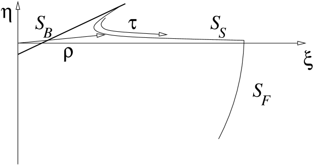
Figure 1: Sketch of the computational domain and of the notation adopted.

where $\tau$ is the arclength measured along the free surface (Fig. 1).

By combining all equations together, we arrive at the new boundary value problem

$$\nabla^{2}\varphi = 0\qquad\qquad\qquad\varOmega$$ (19)

$$\varphi_{\xi} = 0\qquad\qquad\qquad\xi=0$$ (20)

$$\varphi_{\nu} = \cos\gamma\qquad\qquad\qquad\eta=-1+\xi\tan\gamma$$ (21)

$$\varphi = S+\frac{1}{2}\rho^{2}\qquad\qquad h(\xi,\eta)=0$$ (22)

$$S_{\tau} = \pm\sqrt{-2S}\qquad\qquad h(\xi,\eta)=0$$ (23)

$$S_{\nu} = 0\qquad\qquad\qquad h(\xi,\eta)=0$$ (24)

$$S \to -\frac{1}{2}\rho^{2}\qquad\qquad\rho\to\infty$$ (25)

solution of which is derived numerically via a pseudo-time stepping procedure discussed in detail in the next section.

3 Iterative Solution Method

The solution of the boundary value problem (19)-(24) is obtained by a pseudo-time stepping procedure similar to that adopted for the solution of the water entry problem in time domain (Battistin & Iafrati, 2003, 2004). The procedure is based on an Eulerian step, in which the boundary value problem for the velocity potential is solved, and a Lagrangian step, in which the free surface position is moved in a pseudo-time stepping fashion and the velocity potential on it is updated.

3.1 Eulerian substep

Starting from a given free surface shape with a corresponding distribution of the velocity potential on it, the velocity potential at any point $\boldsymbol{x}_{P}=(\xi_{P},\eta_{P})\in\>\>\varOmega$ is written in the form of boundary integral representation

$$\varphi(\boldsymbol{x}_{P})=\int_{S_{S}\cup S_{B}\cup S_{\infty}}\left(\frac{\partial\varphi(\boldsymbol{x}_{Q})}{\partial\nu_{Q}}G(\boldsymbol{x}_{P}-\boldsymbol{x}_{Q})-\varphi(\boldsymbol{x}_{Q})\frac{\partial G(\boldsymbol{x}_{P}-\boldsymbol{x}_{Q})}{\partial\nu_{Q}}\right)\mbox{d}S_{Q}\;,$$ (26)

where $\boldsymbol{x}_{Q}=(\xi_{Q},\eta_{Q})\in\>\>\partial\varOmega$. In the integrals, $S_{B}$ and $S_{S}$ denote the body contour and free surface, respectively, $S_{\infty}$ the boundary at infinity and $G(\boldsymbol{x})=\log\left(|\boldsymbol{x}|\right)/2\pi$ the free space Green’s function of the Laplace operator in two-dimensions.

The velocity potential along the free surface is assigned by equations (22) and (23), whereas its normal derivative on the body contour is given by equation (21). In order to derive the velocity potential on the body and the normal derivative at the free surface the limit of equation (26) is taken as $\boldsymbol{x}_{P}\to\partial\varOmega$. Under suitable assumptions of regularity of the fluid boundary, for each $\boldsymbol{x}_{P}\in\>\>\partial\varOmega$ it is obtained

$$\frac{1}{2}\varphi(\boldsymbol{x}_{P})=\int_{S_{S}\cup S_{B}\cup S_{\infty}}\left(\frac{\partial\varphi(\boldsymbol{x}_{Q})}{\partial\nu_{Q}}G(\boldsymbol{x}_{P}-\boldsymbol{x}_{Q})-\varphi(\boldsymbol{x}_{Q})\frac{\partial G(\boldsymbol{x}_{P}-\boldsymbol{x}_{Q})}{\partial\nu_{Q}}\right)\mbox{d}S_{Q}\>.$$ (27)

The above integral equation with mixed Neumann and Dirichlet boundary conditions, is solved numerically by discretizing the domain boundary into straight line segments along which a piecewise constant distribution of the velocity potential and of its normal derivative are assumed. Hence, in discrete form, it is obtained

$$a_{i}\varphi_{i}+\sum_{j=1}^{N_{B}}\varphi_{j}d_{ij}-\sum_{j=N_{B}+1}^{N_{B}+N_{S}}\varphi_{\nu,j}g_{ij}=e_{i}\varphi_{i}-\sum_{j=N_{B}}^{N_{B}+N_{S}}\varphi_{j}d_{ij}+\sum_{j=1}^{N_{B}}\varphi_{\nu,j}g_{ij}\;\;,$$ (28)

where $N_{B}$ and $N_{S}$ indicate the number of elements on the body and on the free surface, respectively, with $(a_{i},e_{i})=(1/2,0)$ if $i\in(1,N_{B})$ and $(a_{i},e_{i})=(0,-1/2)$ if $i\in(N_{B},N_{B}+N_{S})$. In (28) $g_{ij}$ and $d_{ij}$ denote the influence coefficients of the segment $j$ on the midpoint of the segment $i$ related to $G$ and $G_{\nu}$, respectively. It is worth noticing that the when $\boldsymbol{x}_{P}$ lies onto one of the segments representing the free surface, the integral of the influence coefficient $d_{ij}$ is evaluated as the Cauchy principal part. The symmetry condition about the $\xi=0$ axis is enforced by accounting for the image when computing the influence coefficients.

The size of the panels adopted for the discretization is refined during the iterative process in order to achieve a satisfactory accuracy in the higly curved region about the jet root. Far from the jet root region, the panel size grows with a factor which is usually 1.05.

The linear system (28) is valid provided the computational domain is so wide that condition (15) is satisfied at the desired accuracy at the far field. A significant reduction of the size of the domain can be achieved by approximating the far field behaviour with a dipole solution. When such an expedient is adopted, a far field boundary $S_{F}$ is introduced at a short distance from the origin, along which the velocity potential is assigned as $C_{D}\varphi_{D}$ where $\varphi_{D}$ is the dipole solution

$$\varphi_{D}=\frac{\eta}{\xi^{2}+\eta^{2}}\;\;.$$

Along the boundary $S_{F}$, the normal derivative is derived from the solution of the boundary integral equation. Let $N_{F}$ denote the number of elements located on the far field boundary, the discrete system of equations becomes

$$a_{i}\varphi_{i}+\sum_{j=1}^{N_{B}}\varphi_{j}d_{ij}-\sum_{j=N_{B}+1}^{N_{B}+N_{S}+N_{F}}\varphi_{\nu,j}g_{ij}+C_{D}\sum_{j=N_{B}+N_{S}+1}^{N_{F}}\varphi_{D,j}d_{ij}=e_{i}\varphi_{i}-$$

$$\sum_{j=N_{B}+1}^{N_{B}+N_{S}+N_{F}}\varphi_{j}d_{ij}+\sum_{j=1}^{N_{B}}\varphi_{\nu,j}g_{ij}\;\;,$$ (29)

where $i\in(1,N_{B}+N_{S}+N_{F})$. An additional equation is needed to derive the constant of the dipole $C_{D}$ together with the solution of the boundary value problem. There is no unique solution to assign such additional condition. Here this additional equation is obtained by enforcing the condition that the total flux across the far field boundary has to equal that associated to the dipole solution, which in discrete form reads (Battistin & Iafrati, 2004)

$$-\sum_{j=N_{B}+N_{S}+1}^{N_{B}+N_{S}+N_{F}}\varphi_{\nu,j}\Delta s_{j}+C_{D}\sum_{j=N_{B}+N_{S}+1}^{N_{B}+N_{S}+N_{F}}\varphi_{D\nu,j}\Delta s_{j}=0\;\;.$$ (30)

The solution of the linear system composed by equations (29) and (30), provides the velocity potential on the body contour and its normal derivative on the free surface. Hence, the tangential and normal derivatives of the modified velocity potential can be computed as

$$S_{\tau}=\varphi_{\tau}-\rho\rho_{\tau}\qquad,\qquad S_{\nu}=\varphi_{\nu}-\rho\rho_{\nu}$$ (31)

allowing to check if the kinematic condition on the free surface (24) is satisfied. Unless the condition is satisfied at the desired accuracy, the free surface shape and the distribution of the velocity potential on it are updated and a new iteration is made.

3.2 Update of free surface shape and velocity potential

The solution of the boundary value problem makes available the normal and tangential derivatives of $S$ at the free surface. A new guess for the free surface shape is obtained by displacing the free surface with the pseudo velocity field $\nabla S$, which is

$$\frac{D\boldsymbol{x}}{Dt}=\nabla S\;\;.$$ (32)

Equation (32) is integrated in time (actually, it would be more correct to say pseudo time) by a second order Runge Kutta scheme. The time interval is chosen so that the displacement of the centroid in the step is always smaller than one fourth of the corresponding panel size. Once the new shape is available, the modified velocity potential on it is initialized and the velocity potential is derived from equation (22). At the intersection of the free surface with the far field boundary the velocity potential is provided by the dipole solution, by using the constant of the dipole obtained from the solution of the boundary value problem at the previous iteration. The value of the velocity potential is used to compute the corresponding modified velocity potential from equation (22) and then the dynamic boundary condition (23) is integrated along the free surface moving back towards the intersection with the body contour, thus providing the values of $S$ and $\varphi$ on the new guess.

For the wedge entry problem, at the far field, the modified velocity potential behaves as $S\to-\rho^{2}/2$ and thus, $S_{\tau}\simeq-\rho$ as $\rho\to\infty$ (Fig. 1). In this case the boundary condition can be easily integrated along the free surface, in the form

$$S=-\frac{1}{2}(\tau+C)^{2}\;\;.$$ (33)

By assuming that the free surface forms a finite angle with the body contour, the boundary conditions (21) and (24) can be both satisfied at the intersection point only if $S_{\tau}=0$ and thus $S=0$. From equation (33) it follows that the conditions are satisfied if $C=0$ and $\tau$ is taken with origin at the intersection point, i.e.

$$S=-\frac{1}{2}\tau^{2}\;\;.$$ (34)

Although equation (34) holds for the final solution, the conditions are not satisfied for an intermediate solution. In this case, for the new free surface shape the curvilinear abscissa $\tau$ is initialized starting from the intersection with the body contour and the constant $C$ is chosen to match the value of the modified velocity potential at the intersection with the far field boundary. Once the distribution of the modified velocity potential on the free surface is updated, the velocity potential is derived from equation (22), and the boundary value problem can be solved.

Additional considerations are deserved by the choice of $\nabla S$ as pseudo velocity field. It is easy to see that with such a choice, once the final solution has been reached and $S_{\nu}$ approaches zero all along the free surface, the displacements of the centroids are everywhere tangential to the free surface, thus leaving the free surface shape unchanged. However, this is not enough to explain why the use of $S_{\nu}$ as normal velocity drives the free surface towards the solution of the problem. By differentiating twice in $\tau$ equation (33) we have that $S_{\tau\tau}=-1$. From equation (16), it is $S_{\nu\nu}+S{\tau\tau}=-2$ and then on the free surface

$$S_{\nu\nu}=-2-S_{\tau\tau}=-1\;\;.$$

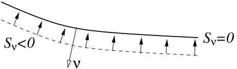
Figure 2: Orientation of the normal velocity field on the free surface guess.

According to the kinematic condition (24) $S_{\nu}=0$ on the free surface, so that if $S_{\nu\nu}<0$ we have $S_{\nu}<0$ in the water domain, which implies that using $S_{\nu}$ as normal velocity drives the free surface towards the solution (Fig. 2).

3.3 Jet modelling

Water entry flows often generates thin sprays along the body contours. An accurate description of such thin layer by a boundary integral representation requires highly refined discretizations, with panel dimensions comparable to the local thickness. Beside increasing the size of the linear system to be solved, the small panel lenghts in combination to the high velocity characterizing the jet region yields a significant reduction of the time step making a detailed description of the solution highly expensive from the computational standpoint.

Despite the effort required for its accurate description, the jet does not contribute significantly to the hydrodynamic loads acting on the body, which is doubtless the most interesting quantity to be evaluated in a water entry problem. Indeed, due to the small thickness, the pressure inside the spray is essentially constant and equal to the value it takes at the free surface, which is $p=0$. This is the reason why rather acceptable estimates of the pressure distribution and total hydrodynamic loads can be obtained by cutting off the thinnest part of the jet, provided a suitable boundary condition is applied at the truncation. In the context of time domain solutions, the cut of the jet was exploited for instance in Battistin & Iafrati (2003) in which the jet is cut at the point where the angle between the free surface and the body contour drops below a threshold value.

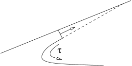
Figure 3: Model adopted for the thin jet and local coordinate system for the shallow water model.

A similar cut can be adopted in the context self-similar problems discussed here. The truncated part is accounted for by assuming that the normal velocity at the truncation of the jet equals the projection on the normal direction of the velocity at the free surface. From the sketch provided in Fig. 3, $\tau^{*}$, which denotes the value of the arclength at the intersection between the free surface and the jet truncation, is different from zero and thus, from equation (34) it follows

$$S_{\tau}(\tau^{*})=-\tau^{*}\;\;.$$ (35)

The value $\tau^{*}$ is derived by initializing the arclength on the free surface as $\tau=\tilde{\tau}+\tau^{*}$ and matching the velocity potential at the far field with the asymptotic behaviour. If the computational domain is large enough, the matching is established in terms of the tangential velocity and thus, from equation (25), we simply get that

$$\tau^{*}=\rho-\tilde{\tau}\;\;.$$

When the dipole solution $C_{D}\varphi_{D}$ is used to approximate the far field solution, $\tau^{*}$ is determined by matching the velocity potential and then, by equations (22) and (34), we get

$$\tau^{*}=(\rho^{2}-2C_{D}\varphi_{D})^{1/2}-\tilde{\tau}\;\;.$$

The tangential velocity at the intersection of the free surface with the jet truncation line can be computed from

$$\varphi_{\tau}=S_{\tau}+\rho\rho_{\tau}\;\;,$$ (36)

where $S_{\tau}$ comes from equation (35). Hence, the normal velocity to be used as boundary condition at the jet truncation is derived as

$$\varphi_{\nu}=\varphi_{\tau}\cos\beta\;\;,$$ (37)

where $\beta$ is angle formed by body contour with the tangent at the free surface taken at the intersection with jet truncation line.

Although very efficient and reasonably accurate, such simplified models do not allow to derive any information in terms of wetted surface and jet speed. An alternative approach, which provides all the information in a rather efficient way, exploits the shallowness of the jet layer. In order to explain the model, it is useful to consider the governing equations in a local frame of reference with $\lambda$ denoting the coordinate along the body and $\mu=f(\lambda)$ the local thickness (Fig. 3). The kinematic boundary condition (24) becomes

$$S_{\mu}=S_{\lambda}f_{\lambda}\qquad\mbox{on }\;\mu=f(\lambda)\;\;.$$ (38)

From the definition (16), it follows that $\nabla^{2}S=-2$. Integration of the above equation across the jet thickness, i.e. along a $\lambda=const$ line, provides

$$\int_{0}^{f(\lambda)}S_{\lambda\lambda}(\lambda,\mu)\mbox{d}\mu+\left[S_{\mu}(\lambda,\mu)\right]_{\mu=0}^{\mu=f(\lambda)}=-2f(\lambda)\;\;.$$ (39)

By exploting the body boundary conditions on the body surface, we finally get (Korobkin & Iafrati, 2006)

$$\frac{\mbox{d}}{\mbox{d}\lambda}\int_{0}^{f(\lambda)}S_{\lambda}(\lambda,\mu)\mbox{d}\mu=-2f(\lambda)\;\;,$$ (40)

which can be further simplified by neglecting the variations of the modified velocity potential across the jet layer, thus arriving to

$$\left[\tilde{S}_{\lambda}(\lambda)f(\lambda)\right]_{\lambda}+2f(\lambda)=0\;\;,$$ (41)

where $\tilde{S}(\lambda)=S\left(\lambda,f(\lambda)\right)\simeq S(\lambda,\mu)$. In terms of $\tilde{S}(\lambda)$ the kinematic condition (38) reads

$$\tilde{S}_{\lambda}=-\frac{S_{\tau}}{\sqrt{1+f_{\lambda}^{2}}}$$ (42)

Equations (41) and (42), together with the dynamic boundary condition (34) can be used to build an iterative, space marching procedure which, at the jet root, matches the solution provided by the boundary integral formulation in the bulk of the fluid. The most relevant point of the procedure are discussed here, whereas a more detailed description can be found in Korobkin & Iafrati (2006).

By using a finite difference discretization of equation (41), the following equation for the jet thickness is obtained

$$f^{k}(i+1)=\omega f^{k-1}(i+1)-(1-\omega)f(i)\left[\frac{\Delta\lambda-\tilde{S}_{\lambda}(i)}{\Delta\lambda+\tilde{S}^{k-1}_{\lambda}(i+1)}\right]\;\;.$$ (43)

As $\tilde{S}_{\lambda}(i+1)$ and $f(i+1)$ are both unknown, the solution is derived by subiterations. In equation (43) $k$ is the subiteration number and $\omega$ is a relaxation parameter, which is usually taken as 0.9. Once the new estimate of the local thickness $f^{k}(i+1)$ is available, it is used in the kinematic condition (42) to evaluate $S^{k}_{\lambda}(i+1)$ as

$$S^{k}_{\lambda}(i+1)=-\frac{S^{k}_{\tau}(i+1)}{\sqrt{1+\left[f_{\lambda}^{k}(i+1)\right]^{2}}}\;\;,$$ (44)

where the derivative of the thickness is evaluated in discrete form as

$$f_{\lambda}^{k}(i+1)=\frac{f^{k}(i+1)-f(i)}{\Delta\lambda}\;\;.$$ (45)

In equation (44) the term $S^{k}_{\tau}(i+1)$ is estimated by exploiting equation (34) which provides $S_{\tau}(i)=-\tau(i)$, and thus

$$S_{\tau}^{k}(i+1)=S_{\tau}(i)+\sqrt{\Delta\lambda^{2}+(f^{k}(i+1)-f(i))^{2}}\;\;.$$ (46)

The system of equations (43)-(46) is solved by subiterations, which use $f(i)$ and $\tilde{S}_{\lambda}(i)$ as first guess values. All quantities at $i=1$ are derived from the boundary integral representation, thus ensuring the continuity of the solution. The spatial step $\Delta\lambda$ is assumed equal to half of the size of the first free surface panel attached to the jet region. Such a choice turns to be useful for the computation of the pressure, as discussed in the next section. The space marching procedure is advanced until reaching the condition $|S_{\lambda}(i+1)|<\Delta\lambda$, which implies that the distance to the intersection with the body contour is smaller than $\Delta\lambda$.

3.4 Pressure distribution

The pressure field on the body can be derived from the distribution of the velocity potential. Let $\varrho$ denote the fluid density, the equation of the local pressure

$$p=-\varrho\left\{\frac{\partial\phi}{\partial t}-\frac{1}{2}\left|\boldsymbol{u}\right|^{2}\right\}\;\;,$$

is written in terms of the self-similar variables (9) thus leading to

$$\psi(\xi,\eta)=-\varphi+(\varphi_{\xi}\xi+\varphi_{\eta}\eta)-\frac{1}{2}(\varphi_{\xi}^{2}+\varphi_{\eta}^{2})\;\;,$$ (47)

where $\psi=p/(\varrho V^{2})$ is the nondimensional pressure.

When the shallow water model is activated, due to the assumptions, the pressure in the modelled part of the jet is constant and equal to the value it takes at the free surface, i.e zero. As a consequence, a sharp drop of the pressure would occur across the separation line between the bulk of the fluid and the modelled part of the jet. In order to avoid such artificial discontinuity, the velocity potential along the body is recomputed by using the boundary integral representation of the velocity potential for the whole region containing both the bulk of the fluid and the part of the jet modelled by the shallow water model. As discussed in the previous section, the spatial step in the space marching procedure of the shallow water model has been chosen as half of the size of the free surface panel adjacent to the modelled part of the jet. This allows a straightforward derivation of the discretization to be used in the boundary integral representation. Two adjacent panels in the shallow water region are used to define a single panel in the discrete boundary integral representation (29). This panel has the velocity potential associated at the mid node connecting the two shallow water elements which constitutes the panel. On the basis of the above considerations, if $N_{SW}$ is the number of steps in the space marching procedure, the inclusion of the modelled part of the jet in the boundary integral representation corresponds to $N_{SW}/2$ panels on the body contour and $N_{SW}/2$ panel on the free surface, with a total of $N_{SW}$ additional equations in (29). As usual, a Neumann boundary condition is applied to the panels lying along the body contour, and a Dirichlet condition is applied to the panels lying on the free surface. It is shown in the following that including the shallow water solution in the boundary integral representation results in a much smoother pressure distribution about the root of the jet, whereas the remaining part is essentially unchanged.

3.5 Porous and perforated contours

The solution procedure is also applicable to problems in which the solid boundary is permeable, provided the boundary condition can be formulated as a function of the pressure. In these case, of course, an accurate prediction of the pressure distribution is mandatory.

Possible examples are represented by porous or perforated surfaces. In a porous surface the penetration velocity depends on a balance between the viscous losses through the surface and the pressure jump, so that, if the $\boldsymbol{V}\cdot\boldsymbol{n}$ is the normal velocity of the contour, the actual boundary condition is

$$\frac{\partial\phi}{\partial n}=\boldsymbol{V}\cdot\boldsymbol{n}-\alpha_{0}p\;\;,$$ (48)

where $\alpha_{0}$ is a coefficient that depends on the characteristics of the porous layer (Iafrati & Korobkin, 2005$b$). In a perforated surface, the flow through the surface is governed by a balance between the inertial terms and the pressure jump. In this case the condition is usually presented in the form Molin & Korobkin (2001)

$$\frac{\partial\phi}{\partial n}=\boldsymbol{V}\cdot\boldsymbol{n}-\chi\sqrt{p/\varrho}\;\;,\qquad\chi^{2}=\frac{2\sigma\kappa^{2}}{1-\kappa}$$ (49)

where $\sigma$ is a dicharge coefficient which is about $0.5$ and $\kappa$ is the perforation ratio, i.e. the ratio between the area of the holes and the total area.

In terms of the self-similar variables, both cases are still described by the system of equations (9)-(15) but for the body boundary condition (12) which is rewritten as

$$\varphi_{\nu}=\cos\gamma-f(\psi)\qquad\eta=-1+\xi t\tan\gamma\;\;,$$ (50)

where $f(\psi)=\alpha_{0}\psi$ and $f(\psi)=\chi\sqrt{\psi}$ for porous and perforated surfaces, respectively.

Examples of water entry flows of porous or perforated bodies are presented in the next section. The important changes operated on the solution by different levels of permeability are clearly highlighted.

4 Applications

4.1 Wedge entry problem

As a first application, the computational method is applied to the water entry with constant vertical velocity of an infinite wedge. An example of the convergence process for a wedge with 10 degrees deadrise angle is shown in Fig. 4.

It is worth noticing that for convenience, in the wedge entry problem, the first guess for the free surface is derived from the dipole solution at the far field. Indeed, if $C_{D}\varphi_{D}$ approximates the far field behaviour, then the free surface elevation should behave as

$$\eta(0)=\frac{C_{D}}{3\xi^{2}}\;\;,$$ (51)

where the constant $C_{D}$ is derived together with the solution of the boundary value problem, as discussed in section 3. Note that, a few preliminary iterations are performed in order to get a better estimate of the constant $C_{D}$. During these preliminary iterations the free surface varies only due to the variation of the coefficient $C_{D}$ in equation (51).

Once the pseudo time stepping procedure starts, it gradually develops a thin jet along the body surface. When the angle formed by the free surface with the body surface drops below a threshold value, usually 10 degrees, the jet is truncated or the shallow water model is activated. This process is shown in the left picture of Fig. 4 where, for the sake of clarity, the shallow water region is not displayed.

The convergence in terms of pressure distribution is shown in Fig. 5 along with a close up view of the jet root region. It can be noticed that the use of the shallow water solution within the boundary integral representation makes the pressure very smooth about the transition.

Due to the use of the $\nabla S$ as a pseudo velocity field for the displacement of the free surface panels, the achievement of convergence implies that there is no further motion of the free surface in the normal direction, and thus the kinematic condition (17) is satisfied. A more quantitative understanding of the convergence in terms of the kinematic condition is provided by the quantity

$$K=\int_{S_{S}}S_{\nu}^{2}\mbox{ d}s\;\;.$$ (52)

The behaviour of $K$ versus the iteration number is displayed in Fig. 6, which indicates that $K$ diminishes until reaching a limit value that diminishes when refining the discretization.

$\gamma$	$C_{p}=2\psi$		$\eta_{max}$
	Present	ZF	Present	ZF
7.5	140.1	140.59	0.5601	0.5623
10	77.6	77.85	0.5538	0.5556
20	17.7	17.77	0.5079	0.5087
30	6.86	6.927	0.4217	0.4243
40	3.23	3.266	0.2946	0.2866

Table 1: Comparison between the results provided by the present solver and the corresponding data derived by the self-similar solution in Zhao & Faltinsen (1993).

In Fig. 7 the free surface profiles obtained for different deadrise angles are compared. In the figure, two solutions, largely overlapped, are drawn for the 10 degree wedge which refers to two different discretizations, with minimum panel size of 0.04 and 0.01 for the coarse and fine grids, respectively. Similarly, two solutions are drawn for the 60 degrees case, one which makes use of the shallow water model and a second solution in which the jet is described by the boundary integral representation. At such deadrise angles, the angle at the tip, which is about 15 degrees, is large enough to allow an accurate and still efficient description of the solution within the standard boundary integral representation.

It is worth noticing that, as the solution is given in terms of the self-similar variables (9), the length of the jet in terms of those variables

$$l_{j}=\sqrt{\xi_{j}^{2}+\eta_{j}^{2}}\;\;,$$ (53)

is also an index of the propagation velocity of the tip. For the present problem, according to equations (9) the scaling from the self-similar to the physical variables is simply linear and thus the $l_{j}$ is just the tip speed. The jet length versus the deadrise angle, which is drawn in Fig. 8, approaches a $1/\gamma$ trend for $\gamma\leq 30$ degrees.

A comparison of the pressure distribution obtained for different deadrise angles is provided in Fig. 9. The results show that, up to 40 degrees deadrise angle, the pressure distribution is characterised by a pressure peak occurring about the root of the jet whereas, at larger deadrise angles, the maximum pressure occur at the wedge apex. As for the free surface shape, also for the pressure distribution two solutions are drawn for the cases at 10 and 60 deadrise angles, which are essentially overlapped.

For validation of the results, some relevant quantities are extracted and compared with corresponding data computed by the Dobrovol’skaya (1969) model in Zhao & Faltinsen (1993). The comparison is established in terms of the maximum pressure coefficient, which is $2\psi_{max}$, and of the vertical coordinate of the point along the body where the pressure gets the peak, $\eta_{max}=\xi_{max}\tan\gamma-1$. The comparison, shown in Table 1, displays a rather good agreement for all the deadrise angles.

When the body surface is either porous or perforated, a flow through the solid boundary occurs which grows with the local pressure. As shown in Fig. 9, for deadrise angles smaller than 40 degrees the pressure takes the maximum at the root of the jet, and this causes a shrinking, and a subsequent shortening, of the jet. The changes in the free surface shape caused by the porosity of the surface on a 10 degrees wedge are shown in Fig. 10 where the shrinking of the jet is clearly highlighted. From the corresponding pressure distributions, which are given in the left picture, it can be seen that even low porosity levels provide an important reduction in the pressure peak, and the peak itself is shifted down towards the wedge apex, thus leading to a shortening of the region of the body exposed to the pressure. Beside the reduction of the peak value, the pressure displays a significant reduction also in the remaining part of the body, and all those effects combined together implies an significant reduction of the total load acting on the body.

Similar results are shown also for a 30 degrees wedge, in Fig. 11, where solutions for perforated surfaces are compared. Quantitatively, the differences in terms of $C_{p}$, $\eta_{max}$ and $l_{j}$ when varying the porous or the perforation coefficient are provided in Table 2.

$\alpha_{0},\chi$	Porous			Perforated
	$C_{p_{max}}$	$\eta_{max}$	$l_{j}$	$C_{p_{max}}$	$\eta_{max}$	$l_{j}$
0.0	6.86	0.4217	5.6612	6.86	0.4217	5.6612
0.02	6.59	0.4052	5.5527	6.69	0.4098	5.5930
0.05	6.20	0.3807	5.4086	6.43	0.3988	5.4910
0.10	5.68	0.3451	5.2084	6.02	0.3697	5.3350
0.20	4.88	0.2887	4.9145	5.33	0.3127	5.0610
0.30	4.28	0.2442	4.7100	4.74	0.2686	4.8339
0.40	3.83	0.2150	4.5610	4.24	0.2285	4.6462
0.50	3.45	0.1856	4.4460	3.81	0.1956	4.4912

Table 2: Effect of the porosity coefficient and of the perforation ratio on some relevant parameters for a 30 degrees wedge.

4.2 Sliding block

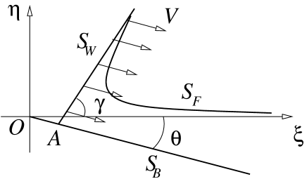
Figure 12: Block sliding along an inclined sloping bed.

As a second application, the method is adopted to study the flow generated when a solid block slides along a sloping bed (Fig. 12). This flow configuration resembles that generated at coastal sites when massive land slides along the sea bed giving rise to tsunamis. The study can help in understanding which are the conditions in terms of the angle of the front and bed slope which result in the larger velocities. The possibility of accounting for the permeability of the mass is exploited as well.

This problem and all the physical implications were already addressed and discussed in Iafrati et al. (2007). As explained in the introduction, the application is here shortly reviewed, focusing the attention on the changes to be operated to the boundary value problem formulated above. Some other aspects of the solutions are highlighted as well.

By assuming a constant entry velocity, which is acceptable in an early stage, the flow is self-similar and can be described by the same approach presented above. The only difference concerns the boundary conditions on the bed and on the front which are

$$\varphi_{\nu}=0\qquad\mbox{ on }\;\eta=-\xi\tan\theta$$ (54)

and

$$\varphi_{\nu}=\sin(\gamma+\theta)-f(\psi)\qquad\mbox{ on }\;\eta=\xi\tan\gamma-\frac{\sin(\gamma+\theta)}{\cos\gamma}$$ (55)

where, as aforesaid, $f(\psi)$ accounts for the permeability of the block and $\theta$ is the inclination of the sea bed (Fig. 12). In this case the solid boundary is represented by both the bed and the block front, but only the latter can be permeable.

The free surface profiles generated by a block sliding over sea beds with different slopes and different inclinations of the block are shown in Fig. 13. When the shallow water model is exploited, the free surface portions belonging to the bulk of the fluid and to the shallow water region are displayed, along with the boundary between the two domains. For the case with $\gamma=60$ degrees, the results indicate that the jet length grows, i.e. the tip moves faster, when the beach slope increases from 10 to 40 and decays for larger slopes. Results are similar for the case $\gamma=90$ degrees, although the maximum is achieved for a bed slope of $30$ degrees. For an inclination of the front of $120$ degrees the results show that the jet length decays monotonically as the beach slope increases. Quantitatively, the results are summarized in Table 3.

$\theta$	$\gamma=60$			$\gamma=90$			$\gamma=120$
	$\xi_{T}$	$\eta_{T}$	$l_{J}$	$\xi_{T}$	$\eta_{T}$	$l_{J}$	$\xi_{T}$	$\eta_{T}$	$l_{J}$
10	1.822	1.277	1.474	0.9848	1.196	1.196	0.3894	0.8576	1.232
20	2.003	1.500	1.732	0.9397	1.261	1.261	0.2940	0.7764	1.163
30	2.097	1.631	1.884	0.8660	1.249	1.249	0.2039	0.6468	0.8670
40	2.112	1.689	1.951	0.7660	1.176	1.176	0.1182	0.4794	0.6211
50	2.056	1.682	1.942	0.6428	1.050	1.050	4.8543E-02	0.2632	0.3309
60	1.931	1.613	1.863	0.5000	0.8749	0.8749

Table 3: Coordinates of the jet tip $(\xi_{T},\eta_{T})$ and length of the jet $l_{J}$ for a block with $\gamma=60,90$ and $120$ degrees sliding along a seabed with different slopes.

In the case of a permeable front, the flow across the solid boundary makes the jet thinner and shorter, i.e. the tip speed is lower. This can be seen from Fig. 14 where the free surface profiles obtained for a perforated block with $\gamma=90$ degrees and $\theta=40$ are shown for $\chi=0,0.1$ and $0.2$.

4.3 Floating plate impact

The computational procedure can be also applied in contexts in which the problem is not strictly self-similar but is can be approximated as self-similar under additional assumptions. This is for example the case of the sudden start of a wedge originally floating on the free surface with the apex submerged (Iafrati & Korobkin, 2005$a$) or the sudden start of a floating wedge in a weakly compressible liquid (Korobkin & Iafrati, 2006). Both problems are approximately self-similar in the small time limit. It can be shown that the problems can be represented by the same boundary value problem, aside from some differences in the coefficients appearing in the dynamic boundary condition (13) or (23).

As a particular example, the water entry of a floating plate is presented here below. Formally, the plate entry problem is not self-similar as the breadth of the plate introduces a length scale. By formulating the solution of the problem in the form of a small time expasion, it can be shown that the first order solution is singular at the edge of the plate. In order to resolve the singularity, an inner solution has to be formulated under set of stretched coordinates. Hence, the inner solution has to be matched to the outer one at the far field.

It is worth remarking that a detailed derivation of the outer and inner problems, as well as the matching condition, can be found in Iafrati & Korobkin (2004) whereas practical applications are discussed in Iafrati & Korobkin (2008) and Iafrati & Korobkin (2011). The problem is here discussed in order to highligth the different form of the dynamic boundary condition compared to the previous cases. This requires a different procedure as the dynamic boundary condition cannot be integrated analytically and, moreover, an additional unknown appears which has to be derived as a part of the solution. As shown in the following, the additional unknown governs the shape of the free surface.

Within a small time assumption, the problem in a close neighbourood of the edge is formulated in terms of the following variables:

$$\xi=\frac{x-1}{Bt^{2/3}}\qquad\eta=\frac{y}{Bt^{2/3}}\qquad\varphi=\frac{\phi}{\sqrt{2B}t^{1/3}}\;\;,B=(9/2)^{1/3}\;\;.$$ (56)

In terms of the new variables, the problem is such that the plate is fixed and the flow is arriving from the far field. As $t\to 0$, in terms of the stretched coordinates (56), the plate occupies the negative $\xi$-axis, with the plate edge located at the origin of the coordinate system. With respect to the pure self-similar problem, some differences occur in terms of the boundary conditions, which are

$$\varphi_{\nu} = 0\qquad\qquad\qquad\xi<0,\eta=0$$ (57)

$$S_{\tau} = \pm\sqrt{\frac{1}{2}\rho^{2}-S}\qquad\qquad h(\xi,\eta)=0$$ (58)

$$h(0,0) = 0\;,\;h_{\xi}(0,0)=0\qquad\qquad(\xi=0,\eta=0)$$ (59)

$$\varphi \to \sqrt{\rho}\sin(\delta/2)\qquad\qquad\rho\to\infty$$ (60)

where equations (59) states that the free surface is always attached at the plate edge, and leaves the plate tangentially (Iafrati & Korobkin, 2004).

Although the solution procedure is quite similar to that presented above, there are some important differences which deserve a deeper discussion. Due to the different coefficients in the dynamic boundary condition, it cannot be analytically integrated along the free surface. Equation (58) is integrated numerically along the free surface starting from the far field where the matching with the asymptotic behaviour of the solution is enforced. The numerical integration needs care, in particular at large distances from the origin, in order to avoid the effects of round off errors. Aside from that, the problem is even more complicated as the sign in the dynamic boundary condition (58) changes along the free surface. This can be easily understood by examining the behaviour of the solution nearby the plate edge, $\rho\to 0$, and in the far field as $\rho\to\infty$. Close to the edge, the flow exits from the area beneath the plate toward the free surface. If $\tau$ denotes the arclength along the free surface, oriented toward the far field, we have that $\varphi_{\tau}>0$, and thus, as $\rho=0$ at the edge, $S_{\tau}>0$. At the far field, the free surface approach the undisturbed water level and thus, from the definition (22) it follows that $S_{\tau}\to-\rho$.

The position of the inversion point, i.e. the point where the sign in the dynamic condition changes from negative to positive, is unknown and has to be determined as a part of the solution. The additional constraint given by equations (59) is used to that purpose. In discrete form, at each time step, three distributions of the velocity potential are initialized on the free surface by locating the inversion point at the same panel vertex used at the previous step, and at the vertices of the preceeding and successive panels. Three boundary value problems are solved by using the three distributions of the potential and the three values of the normal derivatives of the velocity potential at the first panel attached at the plate are compared. The inversion point is located at that position among the three, which yields the smallest value of the normal velocity at the plate edge (Iafrati & Korobkin, 2004).

Physically, the inversion point represents a point of discontinuity in the tangential velocity along the free surface. Indeed, such a point is the tip of the thin splash developing at short distance from the edge. The discontinuity in the tangential velocity is associated to the discontinuity in the tangent to the free surface at the tip. Due to the lack of a known surface to be used as a base for the shallow water model, in this case the flow within the thin splash is described by the boundary integral representation, aside from the very thin part which is cut off. The discretization is continuously refined in order to ensure an adequate resolution throughout the spray, whereas the normal velocity at the trucation is assigned to be equal to the projection of the velocities at the two sides of the free surface along the normal to the truncation panel.

In Fig. 15 the convergence history of the free surface profiles is shown, along with a comparison of the final free surface shape with experimental data (Yakimov, 1973). In order to make more evident the differences in the curves, a different scale is used for the horizontal and experimental axes in the picture with the convergence history. In establishing the comparison with the experimental data, the points digitalized by the original paper are assumed with origin at the plate edge and are scaled by the same factor in both directions, with the scale factor chosen to reach the best overlapping at the root of the spray.

Once the convergence is achieved, the distribution of the velocity potential along the body can be used to derive the pressure on the plate. Starting from the definition of the stretched variables, the pressure can be defined as $p/\varrho=1/Bt^{-2/3}\psi$, where

$$\psi=-\varphi+2(\xi\varphi_{\xi}+\eta\varphi_{\eta})-(\varphi_{\xi}^{2}+\varphi_{\eta}^{2})\;\;,$$ (61)

the first two contributions originating from the time derivative and the third one related to the squared velocity term. It is worth noticing the differences in the coefficients with respect to those found in the effective self-similar problem (47).

Whereas a more detailed discussion on the behaviour of the pressure and the matching between inner and outer solutions is provided in Iafrati & Korobkin (2008, 2011), here the attention is focussed on the pressure $\psi$ given in terms of the inner variables. The pressure, which is shown in Fig. 16, displays a peak located at a short distance from the edge and a sharp drop to zero at the plate edge. On the other side, the pressure gently diminishes approaching the outer solution.

4.4 Ditching plate

As a last example, the solution method is applied to derive the self-similar solution characterizing the water entry of a two-dimensional plate with a high horizontal velocity component, which is considered as an exemplification of the aircraft ditching problem. There are two parameters governing the solution in this case, which are the velocity ratio $V/U$ and the angle $\gamma$ formed by the plate with the still water level.

The problem is self-similar under following set of variables

$$\xi=\frac{x}{Ut}\qquad\eta=\frac{y}{Ut}\qquad\varphi=\frac{\phi}{U^{2}t}\;\;,$$ (62)

where $U$ and $V$ are the horizontal and vertical velocity of the plate. In terms of the variables (62), the plate edge is located at $(1,V/U)$. The governing equations are about the same as (19)-(25), aside from the symmetry condition, which does not hold in the ditching case. The boundary condition on the body is

$$\varphi_{\nu}=\sin\gamma+\frac{V}{U}\cos\gamma\qquad\eta=-\frac{V}{U}+(\xi-1)\tan\gamma\;\;.$$ (63)

As for the plate entry problem, also in this case an additional condition is enforced at the edge, requiring that the free surface is always attached to the edge and that the free surface leave the plate tangentially. The solution on the left hand side is then rather similar to that of the plate entry case, with the dynamic boundary condition changing the sign at some inversion point. The position of the inversion point is determined by enforcing the two additional conditions at the plate edge.

In Fig. 17 the solution is shown in terms of free surface shape for a plate with $\gamma=10$ degrees and a velocity ratio $V/U=0.03$. The solution displays the very thin jet developing along the plate. According to the definition of the stretched variables (62), the tip of the jet moves with a velocity which is about three times the velocity of the plate. With similar considerations, the root of the jet, which is just in front of the pressure peak, moves with a horizontal velocity which is about 1.5 times the horizontal velocity of the plate.

Beside the thin jet developing along the plate, a splash is formed at the rear. Differently from that found for the vertical entry case, the splash is much milder and much thicker, with a rather large angle formed by the two sides of the free surface at the tip. For the case presented here, the tip of the splash is located at $(-0.029,0.099)$, and the free surface is inclined of about 52 and 67 degrees with respect to the still water level on the left and right hand side, respectively. This result in an internal angle of about 61 degrees.

The pressure distribution for the same case is plotted in Fig. 18, where $\psi=p/(\varrho U^{2})$. The pressure peak is located at $\xi\simeq 1.49$, and thus the distance to the plate edge is $0.49/\cos 10\simeq 0.4976$. In the physical variables this means that in a frame of reference attached to the body, the peak moves along the body surface with a velocity equal to $0.4976U$.

Another important information that can be derived by the pressure distribution is the total hydrodynamic load acting on the plate. By integrating the pressure distribution it is obtained that

$$F=\int p{\mbox{d}}s=(\varrho U^{3}t)\int\psi{\mbox{d}}\tau$$

where $\tau$ is the arclength measured along the body in the self-similar plane. From the numerical integration of the pressure distribution along the wetted surface it is obtained that $F\simeq 0.156(\varrho U^{3}t)$.

5 Conclusions

An iterative method for the solution of the fully nonlinear boundary value problems characterizing self-similar free surface flows has been presented. The method has been applied to different examples characterized by different boundary conditions in order to demonstrate the good level of flexibility and accuracy. It has been shown that the method keeps a good accuracy even when dealing with the thin jets developing during water entry processes. In this regard, the shallow water model proved to be very efficient, thus allowing a significant reduction of the computational effort without reducing the level of accuracy.

The applications presented here are all referred to constant velocity. Future extension of the method may involve constant acceleration cases, as that discussed in Needham et al. (2008). In those cases however, additional and more stringent hyphotheses are needed in order to guarantee that gravity and surface tension effects are still negligible.

Figure 4: Convergence of the iterative process for a wedge with 10 degrees deadrise angle. The left picture display the early stage of the process, starting from the initial configuration, till the formation of the thin jet layer (not shown) where the shallow water model is adopted. On the right picture, the convergence process about the root of the jet is shown.

Figure 5: Convergence of the pressure distribution for the 10 degrees wedge. A close up view of the pressure about the jet root is shown, displaying a smooth transition to zero thanks to the use of the shallow water model.

Figure 6: Convergence history of the kinematic boundary condition. The curves refer to two different discretizations, the coarser having a minimum panel size of 0.04, the finer 0.01.

Figure 7: Comparison between the free surface profiles. In the upper picture, solutions refer to $5,7.5,10,20$ degrees deadrise angle. In lower picture, solution refer to $30,40,50,60,70$ and $80$ degrees deadrise angle.

Figure 8: Distance of the jet tip to the wedge apex, versus the wedge angle. According to the definition of self-similar variables (9), $l_{j}V$ represents the velocity at which the tip swept the body surface. The dash line represent the $C/\gamma$ line, where $C=190$ if the angle is expressed in degrees. The graph is given in logscale on the right.

Figure 9: Comparison between the pressure distributions. Solutions for $5,7.5,10,20$ degrees deadrise angle are shown on the left, whereas solutions for $30,40,50,60,70$ and $80$ degrees deadrise angle are given on the right.

Figure 10: Effect of the porosity on the free surface shape and pressure distribution. Solutions are drawn for deadrise angle $\gamma=10$ degree, with porosity coefficients $\alpha_{0}=0,0.02$ and $0.05$.

Figure 11: Free surface shapes and pressure distributions for a wedge $\gamma=30$ degrees deadrise angle in case of perforated surfaces. The perforated coefficients are $0,0.02,0.05,0.10,0.20,0.30,0.40,0.50$.

Figure 13: Free surface profiles for a block, 60 degrees (top), 90 degrees (middle), 120 degrees (bottom). Solutions are drawn for bed slopes 10, 20, 30, 40 and 50 degrees. The line about the jet root indicates the position where the shallow water model is started.

Figure 14: Effect of the permeability of the front on the free surface elevation. Solutions refer to a block front 90 degrees inclination, with $\chi=0$ (solid), $\chi=0.1$ (dash) and $\chi=0.2$ (dot).

Figure 15: On the left, the convergence history of the free surface shape nearby the plate edge is shown. On right, the final solution is compared to the experimental data by Yakimov (1973).

Figure 16: Pressure distribution acting on the plate.

Figure 17: Free surface shape about a ditching plate, 10 degrees deadrise angle. The plate is moving with a velocity ratio $V/U=0.03$. Below, a close up view of the splash tip is provided.

Figure 18: Pressure distribution about a ditching plate, 10 degrees deadrise angle, with velocity ratio $V/U=0.03$.

References

- Battistin & Iafrati (2003) Battistin, D. & Iafrati, A. 2003 Hydrodynamic loads during water entry of two- dimensional and axisymmetric bodies, J. Fluid Struct. 17, 643–664. doi:10.1016/S0889-9746(03)00010-0
- Battistin & Iafrati (2004) Battistin, D. & Iafrati, A. 2004 A numerical model for the jet flow generated by water impact, J. Engng. Math. 48, 353-374. doi: 10.1023/B:engi.0000018173.66342.9f
- Dobrovol’skaya (1969) Dobrovol’skaya, Z.N. 1969 On some problems of similarity flow of fluid with a free surface, J. Fluid Mech. 36, 805-829. doi:10.1017/S0022112069001996
- Faltinsen & Semenov (2008) Faltinsen, O.M. & Semenov, Y.A. 2008 Nonlinear problem of flat-plate entry into an incompressible liquid, J. Fluid Mech. 611, 151-173. doi:10.1017/S0022112008002735
- Iafrati & Battistin (2003) Iafrati, A. & Battistin, D. 2003 Hydrodynamics of water entry in presence of flow separation from chines, Proc. 8th Int. Conf. Num. Ship Hydrod., Busan, Korea.
- Iafrati & Korobkin (2004) Iafrati, A. & Korobkin, A.A. 2004 Initial stage of flat plate impact onto liquid free surface, Phys. Fluids 16, 2214-2227. doi:10.1063/1.1714667
- Iafrati & Korobkin (2005) Iafrati, A. & Korobkin, A.A. 2005 Starting flow generated by the impulsive start of a floating wedge, J. Engng. Math. 52, 99-126. doi:10.1007/s10665-004-3686-9
- Iafrati & Korobkin (2005) Iafrati, A. & Korobkin, A.A. 2005 Self-similar solutions for porous/perfotated wedge entry problem Proc. 20th IWWWFB (available at www.iwwwfb.org), Spitzbergen, Norway.
- Iafrati (2007) Iafrati, A. 2007 Free surface flow generated by the water impact of a flat plate, Proc. 9th Int. Conf. Num. Ship Hydrod., Ann Arbor (MI), USA.
- Iafrati et al. (2007) Iafrati, A., Miloh, T. & Korobkin, A.A. 2007 Water entry of a block sliding along a sloping beach, Proc. Int. Conf. Violent Flows (VF-2007), Fukuoka, Japan.
- Iafrati & Korobkin (2008) Iafrati, A. & Korobkin, A.A. 2008 Hydrodynamic loads during early stage of flat plate impact onto water surface, Phys. Fluids 20, 082104. doi:10.1063/1.2970776
- Iafrati & Korobkin (2011) Iafrati, A. & Korobkin, A.A. 2011 Asymptotic estimates of hydrodynamic loads in the early stage of water entry of a circular disk, J. Engng. Math. 69, 199-224. doi:10.1007/s10665-010-9411-y
- King & Needham (1994) King, A.C. % Needham, D.J. 1994 The initial development of a jet caused by fluid, body and free-surface interaction. Part 1. A uniformly accelerating plate, J. Fluid Mech. 268, 89-101. doi:10.1017/S0022112094001278
- Korobkin & Pukhnachov (1988) Korobkin, A.A & Pukhnachov, V.V. 1988 Initial Stage of Water Impact, Ann. Rev. Fluid Mech. 20, 159-185. doi: 10.1146/annurev.fl.20.010188.001111
- Korobkin & Iafrati (2006) Korobkin, A.A. & Iafrati, A. 2006 Numerical study of jet flow generated by impact on weakly compressible liquid, Phys. Fluids 18, 032108. doi:10.1063/1.2182003
- Mei et al. (1999) Mei, X., Liu, Y. & Yue, D.K.P. 1999 On the water impact of general two-dimensional sections, App. Oc. Res. 21, 1-15. doi:10.1016/S0141-1187(98)00034-0
- Molin & Korobkin (2001) Molin, B. & Korobkin, A.A. 2001 Water entry of a perforated wedge, Proc. 16th IWWWFB (available at www.iwwwfb.org), Hiroshima, Japan.
- Needham et al. (2007) Needham, D.J., Billingham, J. & King, A.C. 2007 The initial development of a jet caused by fluid, body and free-surface interaction. Part 2. An impulsively moved plate, J. Fluid Mech. 578, 67-84. doi:10.1017/S0022112007004983
- Needham et al. (2008) Needham, D.J., Chamberlain, P.G. & Billingham, J. 2008 The initial development of a jet caused by fluid, body and free surface interaction. part 3. an inclined accelerating plate, Q. J. Mech. Appl. Math. 61, 581-614. doi:10.1093/qjmam/hbn019
- Semenov & Iafrati (2006) Semenov, Y.A. & Iafrati, A. 2006 On the nonlinear water entry problem of asymmetric wedges, J. Fluid Mech. 547, 231-256. doi:10.1017/S0022112005007329
- Semenov & Yoon (2009) Semenov, Y.A. & Yoon B.-S. 2009 Onset of flow separation for the oblique water impact of a wedge, Phys. Fluids 21, 112103 (11 pages). doi:10.1063/1.3261805
- Xu et al. (2008) Xu, G.D., Duan, W.Y. & Wu, G.X. 2008 Numerical simulation of oblique water entry of an asymmetrical wedge, Ocean Engng. 35, 1597-1603. doi:10.1016/j.oceaneng.2008.08.002
- Xu et al. (2010) Xu, G.D., Duan, W.Y. & Wu, G.X. 2010 Simulation of water entry of a wedge through free fall in three degrees of freedom, Proc. R. Soc. A 466, 2219-2239. doi:10.1098/rspa.2009.0614
- Yakimov (1973) Yakimov, Y.L. 1973 Influence of atmosphere at falling of bodies on water Izv. Akad. Nauk SSSR, Mekh. Zhidk. 5, 3-7.
- Wu et al. (2004) Wu, G.X., Sun, H. & He, Y.S. 2004 Numerical simulation and experimental study of water entry of a wedge in free fall motion, J. Fluids Struct. 19, 277-289. doi:10.1016/j.jfluidstructs.2004.01.001
- Zhao & Faltinsen (1993) Zhao, R. & Faltinsen, O.M. 1993 Water entry of two-dimensional bodies, J. Fluid Mech. 246, 593-612. doi:10.1017/S002211209300028X