Accelerated Molecular Dynamics through stochastic iterations to strengthen yield of path hopping over upper states (SISYPHUS)
Abstract
We present a new method, called SISYPHUS (Stochastic Iterations to Strengthen Yield of Path Hopping over Upper States), for extending accessible time-scales in atomistic simulations. The method proceeds by separating phase space into basins, and transition regions between the basins based on a general collective variable (CV) criterion. The transition regions are treated via traditional molecular dynamics (MD) while Monte Carlo (MC) methods are used to (i) estimate the expected time spent in each basin and (ii) thermalize the system between two MD episodes. In particular, an efficient adiabatic switching based scheme is used to estimate the time spent inside the basins. The method offers various advantages over existing approaches in terms of (i) providing an accurate real time scale, (ii) avoiding reliance on harmonic transition state theory and (iii) avoiding the need to enumerate all possible transition events. Applications of SISYPHUS to low temperature vacancy diffusion in BCC Ta and adatom island ripening in FCC Al are presented. A new CV appropriate for such condensed phases, especially for transitions involving collective motions of several atoms, is also introduced.
Achieving usefully long timescales (seconds or longer) in atomistic simulations of materials is a problem of great interest, and the search for a practical and general solution has generated intense activity in the field over last several decadesLaio and Parrinello (2002); Voter (1997); Tiwary and van de Walle (2011); Fan et al. (2011); Henkelman and Jonsson (2001); Barkema and Mousseau (1996); Lindorff-Larsen et al. (2011); Lu et al. (2010); Bai et al. (2010) (see Voter et al. (2002); Laio and Gervasio (2008); Perez et al. (2009) for excellent reviews of these and other efforts). The problem arises because, as the system moves from one energy basin to another through infrequent rare events, it stays trapped in some energy basin for extended periods of time. Along with the small time steps (on the order of femtoseconds) needed for the total energy staying conserved, this severely restricts the time scales accessible in MD simulations and also leads to limited phase-space exploration.
Although many methods exist to increase the rate of rare events and efficiently explore the rugged free energy landscape, a frequent limitation is the inability to efficiently obtain an accurate estimate of the “real” time scale of the simulation in general physical systems. Existing schemes to achieve this either
- 1.
-
2.
rely on harmonic approximations to the system’s energy surfaceSørensen and Voter (2000), or
- 3.
In this letter, we propose a new mixed Monte Carlo-Molecular Dynamics method that uses a collective variable (CV) solely to discriminate between basins and transition regions, thus placing very weak requirements on the choice of CV, less stringent than what required in metadynamics methods111In Metadynamics, the CV should distinguish between initial basin, final basin and transition regions. Our CV however is allowed (but not required) to take the same value in two basins.. The method still provides the system’s dynamics via conventional atomic coordinates and thus provides more detailed information than the coarse grained dynamics typically provided by Metadynamics methodsLaio and Parrinello (2002); Bussi et al. (2006). The method also provides an accurate real time scale that does not deteriorate with system size and that does not rely on harmonicity assumptions. There is no need to construct a priori or in situ a catalog of possible transition mechanisms. The method is specially suited for exploiting massive parallel computing.
The proposed algorithm generalizes our previous workTiwary and van de Walle (2011) along multiple dimensions. First, we use a general CV (instead of the system’s potential energy) to discriminate between basins and transition regions and propose a novel type of CV suitable for this purpose in condensed phases. (Recently proposed dimensionality reduction algorithmsTribello et al. (2010, 2012) that discover CV automatically could be used as well.) Second, we introduce an adiabatic switching scheme to efficiently calculate the real time spent inside wells. Finally, we use a more robust criterion to determine when the system has been trapped in a basin for sufficiently long time to have equilibrated therein.
Let the system be characterized by position and velocity . The CV is a function of (we give an example of such a function later in this letter). For a user-specified cut-off value , we define the basins, or wells, W in this -space as a set of connected states for which . In the wells, the method does not follow the system’s exact trajectory in phase space, but instead provides the expected amount of time spent in each well. In contrast, the region of the phase space contains the interesting but infrequently occurring events whose dynamics is fully described. The choice of thus specifies the level of details one wishes to retain in the simulation. Large values of may cause wells to merge and limit the ability to resolve the precise dynamics of some events. The method is still formally correct but the definition of the wells W may not have an an obvious physical meaning. Nevertheless, the method is very robust to changes in that do not change the topology of the well structure (we will provide numerical evidence of this fact).
When the CV of the system is above the threshold , the system evolves via MD according to its true Hamiltonian with constant-pressure (or volume) or constant-temperature (or energy) ensemble as entailed by the simulation. When , the algorithm continues performing MD until either (i) (in which case the system is considered to have exited the well and standard MD continues as described above) or (ii) a time equal to the system’s decorrelation time has elapsed. In that latter case, the system is considered to have been trapped in the well for long enough that it has reached a local thermodynamic equilibrium. This criterion is similar to the one used in other methods Voter (1998); Lu et al. (2010) to define a transition event. At this time, we launch a MC simulation (called MC) whose aim is to generate a new random starting position at the well’s boundary to initialize the next MD episode. MC is run for long enough that the system loses memory of how it entered the well and visits the boundary of the well a few times. MD is restarted with the position where the system last visited the well’s boundary and with velocities drawn from a truncated Maxwell-Boltzmann distribution conditional on (i.e. we only consider velocities in the half-space pointing outwards of the well).
In parallel to the first MC (MC) we perform a second MC run (called MC) that calculates the expected time the system would have spent inside the well. This separation of two MC runs makes our algorithm extremely parallelizable and especially amenable to be used on loosely coupled cluster of computers. We can launch as many MC runs as we have processors available. These runs do not need to communicate with each other, and because of the system’s ergodicity, we can make a quick estimate of the quantity by averaging over these independent runs. This parallelization is even simpler than for the Parallel Replica methodVoter (1998).
Before we describe how we calculate the time the system would have spent in whichever well it visited, we describe specifically how MC is implemented. We define the boundary of the well W with thickness :
| (1) |
Trying to visit with an unbiased potential would be of no avail, since we will rarely visit states in . We thus do MC with a biased potential defined as follows:
| (4) |
Per Eq. (4), MC never visits the outside of the well W and biases states with a penalty function that increases with their depth inside the well. Note that the bias is zero at the well boundary, which is important to obtain the correct sampling distribution of the boundaryVoter (1997). The bias inside the well changes the fraction of time spent at the boundary but not the ratio of the times spent at any two points of the boundary. The parameter determines how sharp the boundary of the well is (a value around 0.5 is found to perform well in practice). is kept around the standard deviation in potential energy of the system. As we demonstrate numerically later, the algorithm is very robust with respect to choice of parameters in Eq. (4).
Having described a way to accelerate the exploration of various wells, we now turn to the question of calculating (via a Monte Carlo labelled MC) the expected time the system would have spent inside well W if there was no acceleration of the dynamics. This time, denoted , can be calculated as the reciprocal of the flux of states exiting the well:
| (5) |
where the average is taken over drawn from the well W with a probability density proportional to . is Boltzmann’s constant, T is the temperature and equals 1 if the event is true and 0 otherwise. denotes the mean projection of a Maxwell-Boltzmann-distributed velocity along the unit vector parallel to , conditional on . When all atoms have the same mass , (a general expression can be found in Ref. Tiwary and van de Walle, 2011).
A straightforward implementation of Eq. (5) will again suffer from a rare event problem. Even an importance sampling scheme, as suggested in Ref. Tiwary and van de Walle, 2011 is not very efficient. Consider what happens if we used the biased potential as defined in Eq. (4) to calculate :
| (6) |
where denote expectations taken under a density proportional to , in which is . This approach is exact in the limit of an ensemble average, but there is a fundamental trade-off that limits its usefulness: A large bias leads to a more rapid convergence of the denominator (due to an increased sampling rate of the boundary) but a slower convergence of the numerator (due to an increase in ).
To avoid this problem, we now propose a technique that bears some resemblance to adiabatic switching methodsFrenkel and Smit (2002); Jarzynski (1997), in which the system is continuously, adiabatically switched from (the true potential) to (identical to the potential used in MC). Let smoothly interpolate between and . Then we can express the ensemble average in Eq.(5) as below (working in terms of rate ):
| (7) | |||||
where denotes a differential volume in 3-N dimensional configuration space for N particles, the integration being performed over entire configuration space within the well W and the expected value in Eq.(7) is defined by
| (8) |
Below we define the term in Eq.(7) and re-express it in a computationally tractable form (see Supplemental Materials (SM) for a more detailed derivation):
We pick a linear switching scheme for , i.e. an interpolation scheme between and :
| (10) |
We now make a few observations regarding Eq.(7). It involves 2 parts. The first is . This is nonzero only when , and whenever it is nonzero, the difference is very small(see Eqs.(1-4)). Since this average is calculated with the maximally biased potential , the boundary is visited frequently, and thus the first term in Eq.(7) can be evaluated very quickly. The second part in Eq.(7) is , where the average does not contain any exponentials that could cause a slow convergence. In SM, we prove rigorously that for this switching scheme and for the choice of biasing potential in Eq.(4) we can use a non-uniform grid to evaluate which can be made finer as but kept coarse for larger , leading to further computational efficiency.
For solid-state systems where bond-breaking is the dominant mechanism of interest, we take to be the bond distortion function (BDF), defined below for a N-particle system:
| (11) |
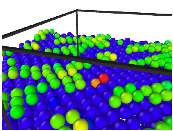
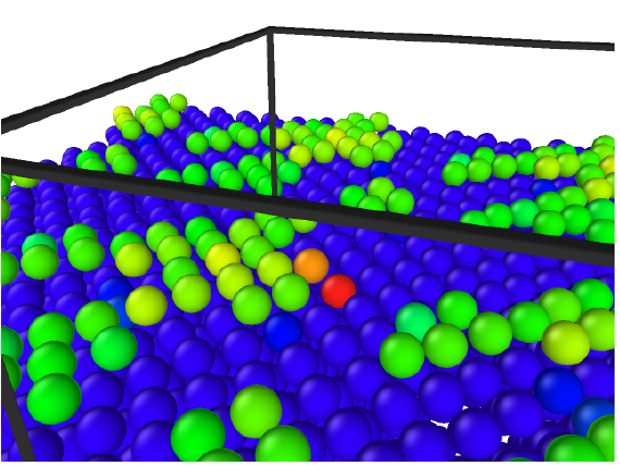
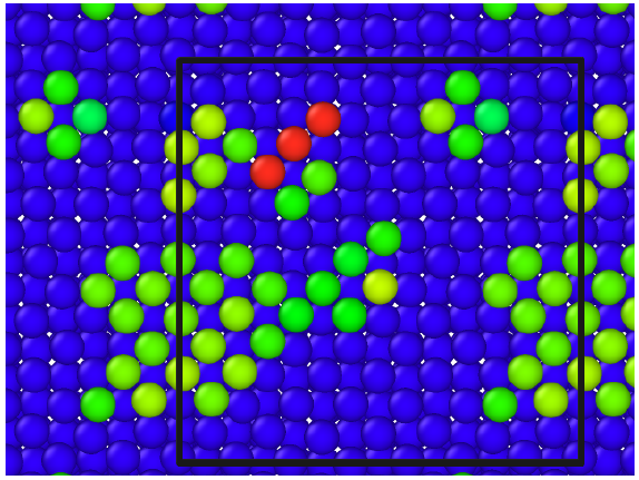
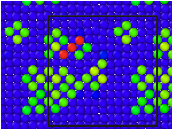
where and is the 0 Kelvin lattice parameter. For each bond, is the equilibrium bond length that can be obtained by a few conjugate gradient steps each time a transition is detected. In the limit that , the BDF, which is a p-norm over fractional bond distortions, approaches the maximum norm, i.e. the strain (times ) in the maximally strained bond. For we thus recover the so-called bond-boost functionFichthorn et al. (2009). We pick around 8-12 for the systems studied in this letter. Not taking allows us to treat on a similar footing cases where (a) one bond is distorted by a large amount, or (b) several bonds are collectively distorted by a significant amount which is however less than the amount in (a). As soon as either (a) or (b) happens, the BDF detects it through a spike and thus we can then switch back to doing completely unbiased MD. This way we can treat transition mechanisms involving small but concerted and collective motion of several atoms (see Fig. 3 g-h)) - for example in glasses, shear transformation zonesFalk and Langer (1998) involve several atoms moving displacing together by a small amount.
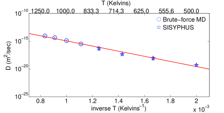
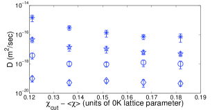
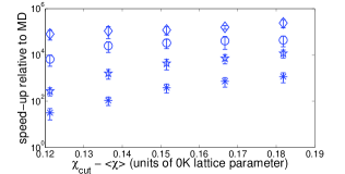
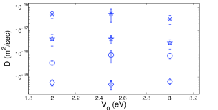
We now describe applications of the algorithm that validate it and demonstrate its insensitivity to choice of parameters. The first example is vacancy assisted lattice diffusion at low temperatures in BCC Tantalum. Lattice diffusion at low temperatures is a problem important in a spectrum of sciences from Materials Science to GeologyMrowec and Marcinkiewicz (1980); Watson and Baxter (2007), but is beyond the time scales one can access in current MD simulations, requiring times longer than millisecondsMendelev and Mishin (2009); Tiwary and van de Walle (2011). We describe the parameters for the MD partAckland and Thetford (1987) of this simulation in SM. In Fig.1 we demonstrate how the diffusion constant through brute-force MD and SISYPHUS for vacancy assisted diffusion lie on the same Arrhenius plot, giving an Arrhenius-type activation energy of 0.9(+/-0.1) eV (in rough agreement with Harmonic Transition State Theory(HTST) calculation of 1.1 eV). Fig.2(top) demonstrates the lack of sensitivity of the dynamics to what and values we pick. As expected the speed-up is higher for higher (Fig.2(middle)). At higher temperature we find slightly higher sensitivity to (still within order of magnitude accuracy). This is because for a low , the values becomes closer to time the system takes to equilibrate in a well. Insensitivity to values can be seen from Fig.2(bottom). A smaller leads to slower sampling in Eq.6, and MC also takes longer to converge. With too high a however, the periphery of the well W can be too steep and one might again face sampling issues since the system can be trapped in some regions of the well boundary. In SM, we provide a back-of-the-envelope estimate of how to pick an optimum for a given system.
For our second application, we studied the room-temperature dynamics of Al adatoms on Al (001) thin film (625 atoms, roughly 3 times larger than the Ta vacancy diffusion example). We picked this problem because firstly, from a technological perspective, it is of immense importance for fabrication processes in nanoscale devices involving growth of thin films from deposited adatomsZhang and Lagally (1997); Becker et al. (2009). This problem is very interesting from a theoretical perspective too, given that it is an inherently non-equilibrium phenomenon dictated by the interplay between kinetics and thermodynamics. Being able to model and control the growth and properties of such films is hugely desirable - the time-scales needed are however far beyond MD. Accurate 0 Kelvin saddle point search methodsHenkelman and Jonsson (1999, 2001) have shown the existence of a large number of transition mechanisms with low and similar activation energies (smaller than 0.4eV). Such low lying barriers can be hard to deal with in most accelerated MD methodsVoter et al. (2002). On-the-fly KMCHenkelman and Jonsson (2001) calculations have been used previously used to get rough estimate of the time-scale for adatom island ripening that we can compare SISYPHUS with. In SM we provide details of the simulation parameters for this system.
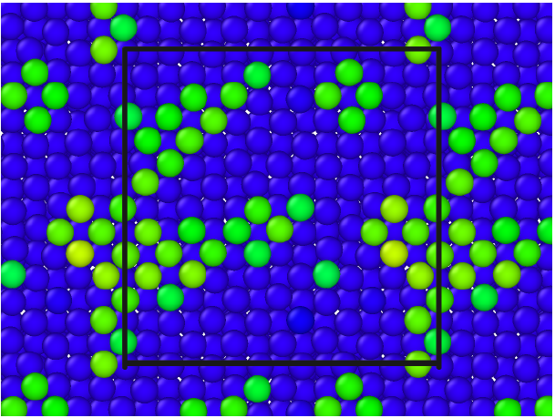
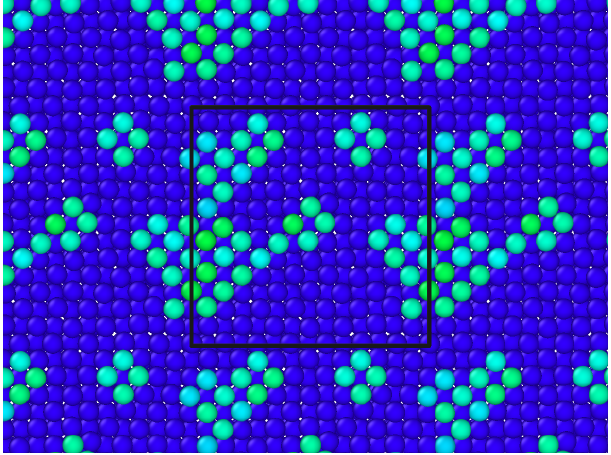
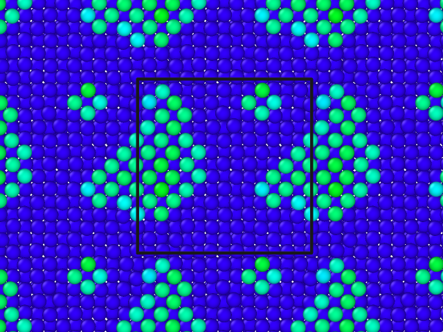
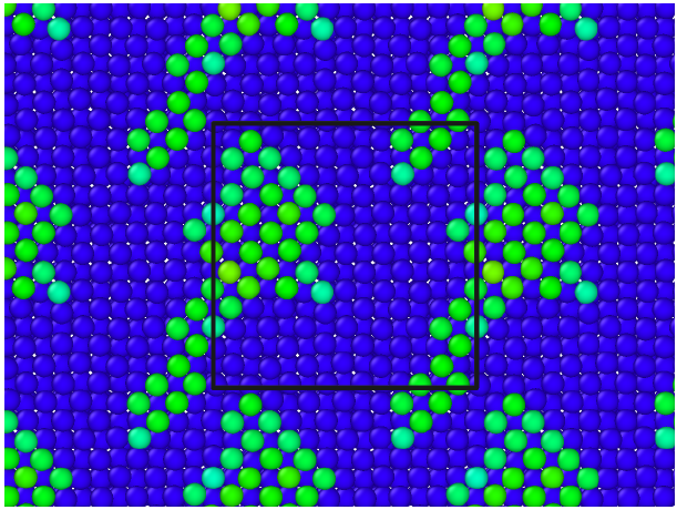
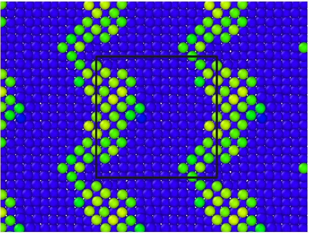
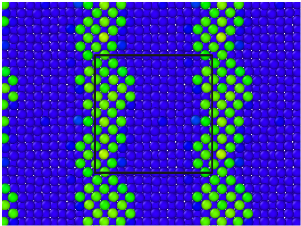
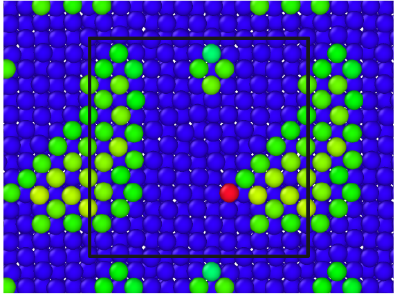
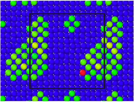
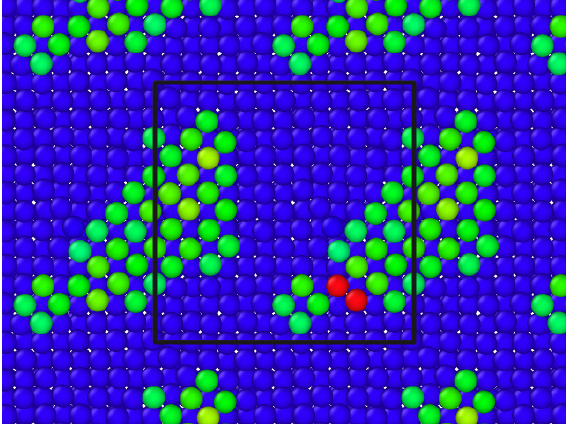
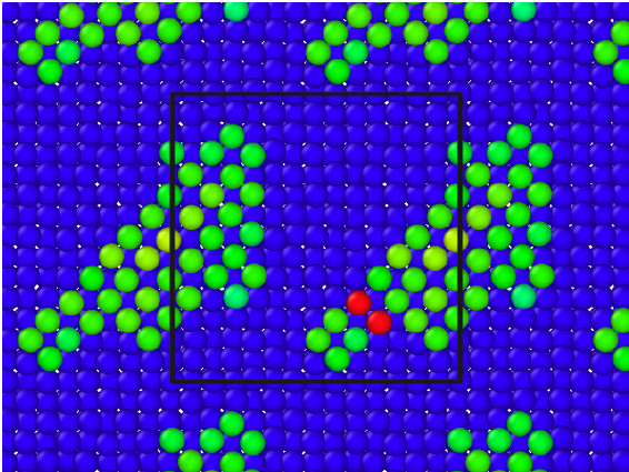
Fig. 3 and the movies in SM illustrate the most common mechanisms seen through SISYPHUS. We have the single adatom hop (a-b), the concerted two adatom hop (c-d), and the concerted event involving an adatom and a substrate atom as the latter moves to the adatom layer (e-f). Occasionally we see more complicated mechanisms like the 3-atom hop (g-h), and events with creation of a vacancy in the top substrate layer (see SM). The first three mechanisms are the most common and are in fact the lowest energy transitions found using the dimer method for saddle point search. In Fig. 4 and movie in SM we show the typical evolution of the island ripening at room temperature over several milliseconds of physical time (exact time can vary from run to run well but still within an order of magnitude). Shown alongwith are corresponding energies obtained by quenching each structure to its local minima, illustrating further the effectiveness of the algorithm in escaping and exploring various local energy minima. The overall time can be compared with the analogous on-the-fly KMC workHenkelman and Jonsson (2001) for same system and interatomic potentialVoter and Chen (1987) where 20 adatoms (half as many as current work) formed one compact cluster around 1ms. As a verification that our proposed BDF is effective to decomposing phase space into disconnected wells, we show, in a movie accompanying the SM, a superposition of snapshots of the system during a MC run, illustrating that the system does not jump from one well to another within one MC run (since it rejects all moves with ).
In conclusion, we have shown SISYPHUS to be an extremely parallelizable and robust set of algorithms that help achieve fraction of second timescale for thousands of atoms. The method works well irrespective of system size, and can be applied in the general setting of any collective variable. We also introduced a new CV appropriate for solid state systems especially for transitions involving collective motions of several atoms.
We would like to thank Dr. Arthur Voter and Prof. Graeme Henkelman for helpful discussions and stimulating the trajectory of this research, Dr. Christopher Weinberger for the HTST calculation for Ta vacancy diffusion, and Prof. Julia Greer for hospitality during PT’s visit to Caltech. This research was supported by the US National Science Foundation through XSEDE computational resources provided by NCSA under grant DMR050013N and DMR120056, and NSF Condensed Matter and Materials Theory program DMR0907669, and the Office of Naval Research through grant N00014-11-1-0886.
References
- Laio and Parrinello (2002) A. Laio and M. Parrinello, Proceedings of the National Academy of Sciences 99, 12562 (2002).
- Voter (1997) A. F. Voter, Phys. Rev. Lett. 78, 3908 (1997).
- Tiwary and van de Walle (2011) P. Tiwary and A. van de Walle, Phys. Rev. B 84, 100301 (2011).
- Fan et al. (2011) Y. Fan, A. Kushima, S. Yip, and B. Yildiz, Phys. Rev. Lett. 106, 125501 (2011).
- Henkelman and Jonsson (2001) G. Henkelman and H. Jonsson, The Journal of Chemical Physics 115, 9657 (2001).
- Barkema and Mousseau (1996) G. T. Barkema and N. Mousseau, Phys. Rev. Lett. 77, 4358 (1996).
- Lindorff-Larsen et al. (2011) K. Lindorff-Larsen, S. Piana, R. O. Dror, and D. E. Shaw, Science 334, 517 (2011).
- Lu et al. (2010) C.-Y. Lu, D. E. Makarov, and G. Henkelman, The Journal of Chemical Physics 133, 201101 (pages 4) (2010).
- Bai et al. (2010) X.-M. Bai, A. F. Voter, R. G. Hoagland, M. Nastasi, and B. P. Uberuaga, Science 327, 1631 (2010).
- Voter et al. (2002) A. Voter, F. Montalenti, and T. Germann, Annual Review of Materials Research 32, 321 (2002).
- Laio and Gervasio (2008) A. Laio and F. L. Gervasio, Reports on Progress in Physics 71, 126601 (2008).
- Perez et al. (2009) D. Perez, B. Uberuaga, Y. Shim, J. Amar, and A. Voter, Annual Reports in Computational Chemistry 5, 79 (2009).
- Sørensen and Voter (2000) M. Sørensen and A. Voter, The Journal of Chemical Physics 112, 9599 (2000).
- Jarzynski (2006) C. Jarzynski, Physical Review E 73, 046105 (2006).
- Bussi et al. (2006) G. Bussi, A. Laio, and M. Parrinello, Phys. Rev. Lett. 96, 090601 (2006).
- Tribello et al. (2010) G. A. Tribello, M. Ceriotti, and M. Parrinello, Proceedings of the National Academy of Sciences 107, 17509 (2010).
- Tribello et al. (2012) G. A. Tribello, M. Ceriotti, and M. Parrinello, Proceedings of the National Academy of Sciences 109, 5196 (2012).
- Voter (1998) A. F. Voter, Physical Review B 57, 13985 (1998).
- Frenkel and Smit (2002) D. Frenkel and B. Smit, Understanding molecular simulation : from algorithms to applications (Academic Press, 2002), 2nd ed., ISBN 0122673514.
- Jarzynski (1997) C. Jarzynski, Phys. Rev. Lett. 78, 2690 (1997).
- Fichthorn et al. (2009) K. A. Fichthorn, R. A. Miron, Y. Wang, and Y. Tiwary, Journal of Physics: Condensed Matter 21, 084212 (2009).
- Falk and Langer (1998) M. L. Falk and J. S. Langer, Phys. Rev. E 57, 7192 (1998).
- Mrowec and Marcinkiewicz (1980) S. Mrowec and S. Marcinkiewicz, Defects and diffusion in solids: an introduction (Elsevier, 1980).
- Watson and Baxter (2007) E. B. Watson and E. F. Baxter, Earth and Planetary Science Letters 253, 307 (2007).
- Mendelev and Mishin (2009) M. I. Mendelev and Y. Mishin, Phys. Rev. B 80, 144111 (2009).
- Ackland and Thetford (1987) G. Ackland and R. Thetford, Philosophical Magazine A 56, 15 (1987).
- Zhang and Lagally (1997) Z. Zhang and M. G. Lagally, Science 276, 377 (1997).
- Becker et al. (2009) K. E. Becker, M. H. Mignogna, and K. A. Fichthorn, Phys. Rev. Lett. 102, 046101 (2009).
- Henkelman and Jonsson (1999) G. Henkelman and H. Jonsson, The Journal of Chemical Physics 111, 7010 (1999).
- Voter and Chen (1987) A. Voter and S. Chen, in Mater. Res. Soc. Proc (1987), vol. 82, pp. 175–180.