Is dark energy evolving?

Abstract

We look for evidence for the evolution in dark energy density by employing Principal Component Analysis (PCA). Distance redshift data from supernovae and baryon acoustic oscillations (BAO) along with WMAP7 distance priors are used to put constraints on curvature parameter $\Omega_{k}$ and dark energy parameters. The data sets are consistent with a flat Universe. The constraints on the dark energy evolution parameters obtained from supernovae (including CMB distance priors) are consistent with a flat $\Lambda$CDM Universe. On the other hand, in the parameter estimates obtained from the addition of BAO data the second principal component, which characterize a non-constant contribution from dark energy, is non-zero at 1$\sigma$. This could be a systematic effect and future BAO data holds key to making more robust claims.

1 Introduction

The late time acceleration of the Universe as suggested by type Ia Supernovae (SNeIa) [1] observations is now confirmed by various different probes [2]. Exploring the physics behind the cosmic acceleration is the focus of next generation surveys. The discovery of an accelerating phase of the Universe poses a very pressing question: what is the driving force responsible for this acceleration and what are its properties. There are two possible ways explored by theorists to answer this question: modify gravity on large scales or invoke a non-standard quantity in the framework of general relativity, commonly termed ‘dark energy’ which has negative pressure [3]. Many theoretical models have been proposed for dark energy, the cosmological constant $\Lambda$ being the simplest, and evolving dark energy scenario explained by using scalar field models [4]. An alternative approach which is complimentary to dark energy model building, is deriving the dark energy properties from the data. The dark energy models are often characterized by the equation of state parameter $w=p/\rho$. For the case of the cosmological constant $w=-1$, and for dynamical models $w$ is a variable. One of the main targets of future Cosmological surveys is to find constraints on the equation of state and also on its evolution (if any).

To quantify the possible dependence of the dark energy properties on redshift, one can either parameterize them or reconstruct them from the data in a non-parametric way. The equation of state is often parameterized as $w=w_{0}+w_{a}(1-a)$. There have been attempts to study the accelerated expansion of the Universe using other kinematic variables like the Hubble parameter $H(z)$, the deceleration parameter $q(z)$, or the jerk parameter $j(z)$ which are all constructed from derivatives of the scale factor $a$ [5]. Direct parameterization has an advantage that one can physically interpret the result easily and quantify the dark energy and other kinematical properties with a few numbers [6, 5]. But this approach can introduce bias in the analysis since the result will always depend on the form of the parameterization chosen [7]. For this reason non-parametric methods have received a lot of attention in the past few years.

Huterer and Starkman were the first to propose the use of Principal component analysis to obtain information about the properties of dark energy [8]. They assumed a fiducial survey with 3000 SNeIa distributed uniformly over a redshift range $0\leq z\leq 1.7$. Using this simulated data set they derived the best determined weight functions for the equation of state $w(z)$. Later Shapiro and Turner used supernovae measurements to analyse the acceleration history assuming a flat spacetime that is homogeneous and isotropic on large scales. Using principal component analysis they found very strong (5$\sigma$) evidence for a period of acceleration and strong evidence that the acceleration has not been constant [9]. Wang and Tegmark proposed a method for measuring the expansion history of the Universe in uncorrelated redshift bins [10]. Zunckel and Trotta used a maximum entropy method based on Bayesian framework to reconstruct the equation of state of dark energy [11]. Sarkar et al., constrained the equation of state of dark energy by using uncorrelated binned estimate and showed that more than three independent parameters of the equation of state can be obtained from future dark energy surveys to an accuracy better than 10$\%$ [12]. Gaussian process (GP) modelling has also been used to reconstruct the dark energy equation of state [13]. Holsclaw et al., used GP modelling and showed that the non-trivial behaviour of $w$ as a function of $z$ can be extracted from future data and they apply their method on SNeIa data to reconstruct the history of the dark energy equation of state out to redshift $z=1.5$ [14]. Ishida et al., used PCA to reconstruct the expansion rate of the universe with SNeIa data [15].

The aim of this work is to find evidence for evolution in the dark energy density. We have used PCA to find constraints on the amplitudes of modes of the dark energy density as a function of redshift [16]. The plan of the paper is as follows: in section 2 we briefly review the parameter degeneracy between the curvature and dark energy and we introduce the data sets used in this work and the methodology in section 3. In section 4 we present our main results and discuss our results in section 5.

2 Parameter constraints and degeneracy

Finding constraints on the dark energy evolution parameters is complicated by the ‘geometric degeneracy’ between dark energy and curvature (see [17] and references therein). It is a common practice to assume spatial flatness to find constraints on dark energy parameters, and a simplified dark energy model is assumed when constraining curvature. For example, if curvature is a free parameter, the equation of state of dark energy is either assumed to be a constant or is parameterized with some simple form: $w(a)=w_{0}+w_{a}(1-a)$. The degeneracy arises, as the observed distances depend both on the expansion history of the Universe and the curvature. As a result it is not possible to constrain both the curvature and dark energy parameters. As also discussed by Mortonson [18] (eq.(17) in the paper), if one uses only distance measurements, then for any value of the spatial curvature, one can derive some dark energy evolution to satisfy the observations. Mortonson used growth data to remove this degeneracy, since unlike the distance data, growth data depends only on the expansion rate. In an attempt to demonstrate that including the curvature as a free parameter is imperative to understand the dark energy evolution, Clarkson et al., showed that the assumption of a flat universe leads to large errors in the reconstruction of the dark energy equation of state even if the true cosmic curvature is very small [19]. Similarly Shafieloo and Linder analysed the degeneracies that arise in the distance-redshift relation when there is no a priori restriction on the equation of state of dark energy [20] and they found that large variation in the parameters are allowed when using only distance measurements.

In this work we assume a homogeneous and isotropic Universe described by the FLRW metric. We keep $\Omega_{k}$ as a free parameter along with the dark energy parameters to be constrained by the data.

3 Methodology and data sets used

3.1 Data sets

The dark energy evolution effects the expansion rate of the Universe and hence the distances on cosmic scales. In this work we have used distance-redshift data from SNeIa and BAO measurements. Listed below are the publicly available data sets used here:

• We use SNeIa Union2.1 sample as described in [21] to estimate the luminosity distance. This sample contains 580 supernovae spanning the redshift range $0.015<z<1.414$.

• BAO data from different galaxy cluster surveys - SDSS ($z$=0.2, 0.35), 6dFGS ($z$=0.106), WiggleZ ($z$=0.44, 0.6, 0.73) and BOSS ($z$=0.57) [22, 23, 24, 25].

In addition to the above data sets we also use the WMAP7 distance priors [26]. The physics at the decoupling epoch ($z_{*}$) affects the amplitude of the acoustic peaks. The evolution of the Universe between now and $z_{*}$ effects the angular diameter distance out to decoupling epoch, and hence the locations of the peaks. This information is encoded in the ‘acoustic scale’ $l_{A},$ and the ‘shift parameter’ $R$ derived from the power spectrum of cosmic microwave background.

3.2 Methodology

The dark energy contribution to the expansion rate is expressed as a sum of two components. The contribution from the first term is constant across the redshift range. The second component corresponds to a variation in dark energy density and hence its contribution varies across the redshift range. We express the second term as a binned expansion, i.e. we divide the redshift range of the data in bins, and given a complete basis set $\{e_{i}\}$, the contribution from the second term can be written in terms of the basis vectors. If the redshift range is divided in, say, $N$ number of bins then every element in the $N\times$1 basis vector can be associated with a redshift bin. The continuum limit is reached as $N\rightarrow\infty$. Thus the dark energy density is expanded as:

$$\rho_{\Lambda}(z)=\rho_{c}\left(\alpha_{0}+\sum_{i=1}^{N}\alpha_{i}e_{i}(z)\right).$$ (3.1)

Here $\alpha_{0}$ specifies the contribution which is constant in redshift and the coefficients $\alpha_{i}$ (for $1\leq i\leq N$) specify the evolution in dark energy density. $\alpha$’s thus determine the dark energy density upto an overall constant $\rho_{c}$ which is the critical energy density today. For $\alpha_{0}=\Omega_{\Lambda}$ and all other $\alpha_{i}$’s = 0, we recover the standard $\Lambda$CDM case. The choice of the basis is arbitrary. We chose the basis vectors so that $e_{i}(z)$=1 in the $i^{th}$ redshift bin and zero otherwise (i.e. we chose the $N$ $\times$ $N$ identity matrix to be the initial basis). In this work the results are produced with $N$=50 bins.

SNeIa: For the standard FLRW metric the luminosity distance is given by

$$d_{L}=\frac{c(1+z)}{\sqrt{|\Omega_{k}|H_{0}^{2}}}~{}S_{k}\left(\sqrt{|\Omega_{k}|H_{0}^{2}}\int_{0}^{z}\frac{dz^{\prime}}{H(z^{\prime})}\right),$$ (3.2)

where $S_{k}(x)$ is equal to $\sin{x}$, $x$, or $\sinh{x}$ corresponding to closed, flat and open Universe and the expansion rate of the Universe is:

$$H(z)=H_{0}[\Omega_{m}(1+z)^{3}+\Omega_{k}(1+z)^{2}+\Omega_{r}(1+z)^{4}+\Omega_{\Lambda}f(z)]^{1/2}.$$ (3.3)

Here $H_{0}$ is the value of the Hubble parameter at present and $f(z)$ captures the form of dark energy evolution. $\Omega_{i}$ is the density parameter, defined as $\Omega_{i}=\rho_{i}(z=0)/\rho_{c}$ and $\Omega_{m}$, $\Omega_{k}$, $\Omega_{r}$ and $\Omega_{\Lambda}$ refer to the contribution in the energy density at the present epoch from matter, curvature, radiation and dark energy respectively and they add to give unity i.e.

$$\Omega_{m}+\Omega_{k}+\Omega_{r}+\Omega_{\Lambda}=1.$$ (3.4)

The value of $\Omega_{r}$ can be neglected in the redshift range corresponding to the supernovae and BAO data. The distance modulus $\mu=m-M$, which is obtained from the Union2.1 compilation can be derived from the luminosity distance as

$$\mu_{th}=5\log_{10}\frac{d_{L}}{Mpc}+25.$$ (3.5)

Here $m$ and $M$ are the apparent and absolute magnitudes respectively. The cosmological parameters are estimated by minimizing the chi-squared merit function:

$$\chi_{{}_{Union2}}^{2}=\sum_{i=1}^{580}\frac{(\mu^{th}(z_{i},p)-\mu^{obs}(z_{i}))^{2}}{\sigma^{2}_{\mu_{i}}},$$ (3.6)

where $p$ is the set of parameters ($\alpha_{i},\Omega_{k},h$).

BAO: Galaxy cluster surveys provide measurements of an angle-averaged distance $D_{V}$

$$D_{V}=\left(\frac{cz(1+z)^{2}d_{A}^{2}}{H(z)}\right)^{\frac{1}{3}},$$ (3.7)

or the distilled parameter $d_{z}=r_{s}(z_{d})/D_{V}$. Here $d_{A}$ is the angular diameter distance which is theoretically given by $d_{L}/(1+z)^{2}$ and $r_{s}(z_{d})$ given by

$$r_{s}(z)=\frac{c}{\sqrt{3}}\int_{0}^{1/1+z}\frac{da}{a^{2}H(a)\sqrt{1+(3\Omega_{b}/4\Omega_{\gamma})a}}$$ (3.8)

is the characteristic scale determined by the comoving sound horizon at an epoch $z_{d}$ slightly after decoupling. This epoch is measured by CMB anisotropy data. We determine $r_{s}(z_{d})$ using the fitting formula given by Percival et al. [23]

$$r_{s}(z_{d})=153.5\left(\frac{\Omega_{b}h^{2}}{0.02273}\right)^{-0.134}\left(\frac{\Omega_{m}h^{2}}{0.1326}\right)^{-0.255}Mpc.$$ (3.9)

Here $\Omega_{b}$ is the baryon density and $h$ is defined as $h=H_{0}/100$ km/s/Mpc. We have 7 BAO points in the redshift range $0.106\leq z\leq 0.73$. Since some of these points are correlated we use the corresponding covariance matrix $C$ and the chi-squared for this data is:

$$\chi_{{}_{BAO}}^{2}=(D)^{T}C^{-1}D$$ (3.10)

where $D=d_{z}^{obs}(z)-d_{z}^{th}(z,p)$ is a column matrix for the seven data points and $p$ is the set of parameters ($\alpha_{i},\Omega_{k},h$).

CMB distance prior: The ‘acoustic scale’ $l_{A}$, the CMB ‘shift parameter’ $R$, and the redshift to decoupling $z_{*}$ mentioned earlier are defined as [26]:

$$l_{A} \equiv (1+z_{*})\frac{\pi d_{A}(z_{*})}{r_{s}(z_{*})},$$ (3.11)

$$R(z_{*}) \equiv \frac{\Omega_{m}H_{0}^{2}}{c}(1+z_{*})d_{A}(z_{*}),$$ (3.12)

$$z_{*} = 1048[1+0.00124(\Omega_{b}h^{2})−0.738][1+g_{1}(\Omega_{m}h^{2})g_{2}].$$ (3.13)

where $g_{1}$ and $g_{2}$ are given by

$$g_{1} = \frac{0.0783(\Omega_{b}h^{2})^{−0.238}}{1+39.5(\Omega_{b}h^{2})^{0.763}}\;,$$ (3.14)

$$g_{2} = \frac{0.560}{1+21.1(\Omega_{b}h^{2})^{1.81}}\;,$$ (3.15)

and the chi-squared can be written as:

$$\chi_{{}_{CMB}}^{2}=(D)^{T}C^{-1}D\;.$$ (3.16)

Here $D$=$(l_{A}^{th}(p)-l_{A}^{obs}$, $R^{th}(p)-R^{obs}$, $z_{*}^{th}(p)-z_{*}^{obs})^{T}$, $C$ is the corresponding covariance matrix and $p$ is the set of parameters ($\alpha_{i},\Omega_{k},h,\Omega_{b}$).

Fisher Matrix and eigenmodes: We assume that our data set is composed of independent observations and is well approximated by a Gaussian probability density. Now since the measurements are independent one can take the product of their corresponding likelihood functions to obtain the combined likelihood function. One can maximise this likelihood function to find the best fit parameters or one can minimize the corresponding chi-squared merit function. The combined chi-squared for all the data sets will be a sum of chi-squares from individual measurements

$$\chi_{{}_{Total}}^{2}=\chi_{{}_{Union2}}^{2}+\chi_{{}_{BAO}}^{2}+\chi_{{}_{CMB}}^{2}.$$ (3.17)

The cosmological parameters in our analysis are as follows: curvature parameter $\Omega_{k}$, the Hubble parameter $h$, dark energy density parameters $\alpha_{i}$’s and the baryon density $\Omega_{b}$. Thus if we have $N$ bins we have $N+$4 unknown parameters. From this chi-square one can construct the Fisher matrix. The Fisher Matrix is defined as the expectation value of the derivatives of the log of the likelihood $L(\propto e^{-(\chi^{2}/2)})$, with respect to the parameters:

$$F_{ij}=-\left\langle\frac{\partial^{2}\ln L}{\partial p_{i}\partial p_{j}}\right\rangle\;.$$ (3.18)

Depending upon the data set under consideration we construct the corresponding Fisher matrix. For this, one has to chose a particular point $p_{0}$ in the parameter space at which the Fisher matrix is evaluated. We chose this point to correspond to the standard $\Lambda$CDM case, $\alpha_{0}=\Omega_{\Lambda}$ and $\alpha_{i}=0$ for $1\leq i\leq N$. Once we have the Fisher matrix, we marginalize over all the parameters other than $\alpha_{i}$ ($1\leq i\leq N$), i.e. $\alpha_{0}$, $\Omega_{k}$, $h$ and $\Omega_{b}$. We are left with a Fisher matrix of the parameters that correspond to the evolution in dark energy density. We diagonalize it so that it can be written as

$$F=W\Lambda W^{T},$$ (3.19)

where the columns of the orthogonal decorrelation matrix $W$, are the eigenvectors of $F$ and $\Lambda$ is a diagonal matrix with the eigenvalues on its diagonal. We can now find a new set of basis functions which is a linear combination of the old basis function $e_{i}$. This new basis set has decorrelated vectors and since these basis functions are orthonormal and complete we can write the contribution of dark energy in terms of these uncorrelated basis vectors $c_{i}$:

$$\sum_{i=1}^{N}\alpha_{i}e_{i}(z)=\sum_{i=1}^{N}\beta_{i}c_{i}(z)\;.$$ (3.20)

The eigenmatrix $W$ is the Jacobian matrix of the transformation of one basis to another, so one can construct these new basis functions $c_{i}(z)$ as (see [27] for details)

$$c_{i}(z)=We_{i}(z)$$ (3.21)

Figure 1: The panel shows the eigenmodes obtained for the Supernovae+CMB data set. Solid (black), dashed (red), dot-dashed (blue) and dotted (purple) curves correspond to the first, second, third and fourth eigenmode respectively.

(a) Part 1

(b) Part 1

Figure 2: The left panel shows the estimates for dark energy parameters. Color scheme (from left to right): Black/square (Case 1): $\alpha_{0}$ $\&$ $\beta_{1}$ allowed to vary, Blue/circle (Case 2): $\alpha_{0}$, $\beta_{1}$ $\&$ $\beta_{2}$ allowed to vary, Red/up arrow (Case 3): $\alpha_{0}$, $\beta_{1}$, $\beta_{2}$ $\&$ $\beta_{3}$ allowed to vary, Green/down arrow (Case 4): $\alpha_{0}$, $\beta_{1}$, $\beta_{2}$, $\beta_{3}$ $\&$ $\beta_{4}$ allowed to vary. The right panel shows the curvature parameter estimates.

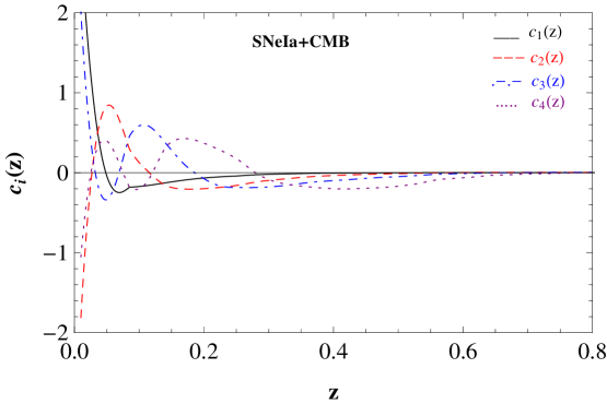
Note that in our case the initial basis set is just the identity matrix. The advantage of this new basis is that the $\beta_{i}$ are uncorrelated, which implies that any pair of coefficients has a non-degenerate error ellipse. These eigenmodes are arranged from the best determined mode to the least determined mode i.e., from the largest to the smallest eigenvalues (the error on these modes goes as $\sigma\propto\lambda^{-1/2}$) and then we choose the first few best determined eigenmodes to reconstruct the dark energy density and carry out the chi-squared minimization. Also note that the constant mode $\alpha_{0}$ is not decorrelated from the rest of the modes and is unaffected by the diagonalisation of Fisher matrix. We show the four best determined eigenmodes for the different data set combinations in the figures below. A non-zero mode amplitude of these principal components would indicate time evolution in dark energy.

The main advantage of the PCA is dimensionality reduction. Initially our parameter space had $N+4$ parameters. Now, depending on the number of principal components chosen for reconstruction, the parameter space would be reduced. The number of principal components to be used for reconstruction depends on how much information are we willing to discard. If we used all the principal components, we would have 100$\%$ information but the uncertainties in our parameter estimates would be too large to have any meaningful interpretation. The sum of all the eigenvalues $\lambda_{i}$ quantifies the total variance in the data and if we use the first $M$ principal components then it encloses $r_{M}$ $\%$ of this variance where

$$r_{M}=100\frac{\sum_{i=1}^{M}\lambda_{i}}{\sum_{i=1}^{N}\lambda_{i}}.$$ (3.22)

4 Results

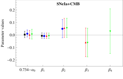
We use Markov chain Monte Carlo (MCMC) method (Metropolis-Hastings MCMC chains) for estimating the parameters and their corresponding errors. We show the best determined eigenmodes for the different dataset combinations. In the plots the different parameter estimates are found by allowing different number of dark energy evolution parameters to vary. First we combine the supernovae measurements with the CMB distance priors and resulting constraints are shown in Figure 2a and 1. Then we add the BAO measurements to this data set to see how they effect the parameter constraints. Following [16] we employ the following trick when evaluating the Fisher matix after the addition of BAO data: we keep $H(z)$ in $d_{z}$ as fixed. If we don’t do this we get spike like features in our eigenfunctions. The results after addition of BAO data are shown in figure 3 and 4a. For plotting convenience, instead of plotting $\alpha_{0}$ we show the difference 0.734 - $\alpha_{0}$ (the WMAP7 constraint on $\Omega_{\Lambda}$ in the $\Lambda$CDM model is $\Omega_{\Lambda}\sim 0.734$). We summarise our main results below:

• In the plots above we present the results obtained by varying different number of principal components for each data set. We observe that the constraint on the curvature parameter $\Omega_{k}$ is robust against variation in the number of principal component chosen for reconstruction. This indicates that the curvature and dark energy evolution parameters have been decorrelated. The results are consistent with a flat Universe.

• The addition of CMB priors is crucial. The analysis using only the distance measurements resulted in a very wide allowed range for $\Omega_{k}$ and the dark energy parameters.

  

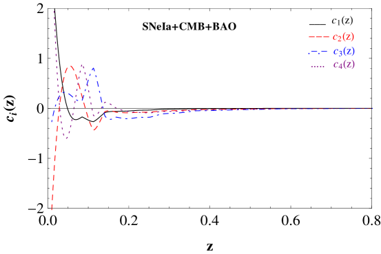
  Figure 3: The panel shows the eigenmodes obtained for the Supernovae+CMB+BAO data set. Solid (black), dashed (red), dot-dashed (blue) and dotted (purple) curves correspond to the first, second, third and fourth eigenmode respectively.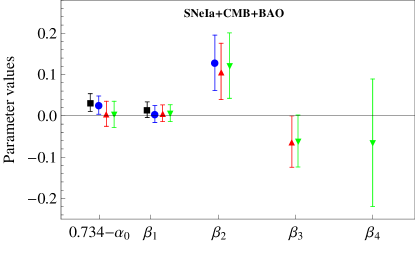

  

  (a) Part 1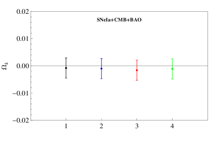

  

  (b) Part 1

  Figure 4: The left panel shows the estimates for the dark energy parameters. Color scheme (from left to right): Black/square (Case 1): $\alpha_{0}$ $\&$ $\beta_{1}$ allowed to vary, Blue/circle (Case 2): $\alpha_{0}$, $\beta_{1}$ $\&$ $\beta_{2}$ allowed to vary, Red/up arrow (Case 3): $\alpha_{0}$, $\beta_{1}$, $\beta_{2}$ $\&$ $\beta_{3}$ allowed to vary, Green/down arrow (Case 4): $\alpha_{0}$, $\beta_{1}$, $\beta_{2}$, $\beta_{3}$ $\&$ $\beta_{4}$ allowed to vary. The right panel shows the curvature parameter estimates.

• The constraints obtained from the supernovae-CMB combined measurements are consistent with a flat $\Lambda$CDM Universe. The first few principal components are consistent with zero. The reconstruction is done using upto 4 principal components. This amounts to incorporating almost 97$\%$ of the information (see 3.22).

• The addition of the BAO data to the supernovae-CMB data set improves the parameter estimates but also changes their value. The reconstruction is done using upto 4 principal components. This amounts to incorporating almost 94$\%$ of the information (see 3.22). The coefficients of the first two eigenmodes are now slightly shifted from zero.

5 Discussion

Finding constraints on both the flatness of the Universe and the dark energy parameters, in models that allow dark energy evolution is difficult because of the geometric degeneracy. Weak assumptions on the possible evolution of dark energy can limit the allowed values of $\Omega_{k}$ and some simple parametrization of the equation of state is often assumed to put simultaneous constraints. But such assumptions/parametrization can introduce significant bias in the analysis and the results obtained. For example Clarkson et al., showed that the assumption of a flat universe leads to large errors in reconstructing the dark energy equation of state even if the true cosmic curvature is very small [19].

In this work we have used a non-parametric method: Principal Component Analysis, to look for evidence for evolution in the dark energy density. The dark energy density is expressed as a sum of two terms: a constant term that accounts for the contribution that is redshift independent and an additional term constructed from the non constant density contribution. This later term is formulated using PCA so that all the parameters obtained have uncorrelated errors and a non constant amplitude of these modes would indicate dark energy evolution. The distance-redshift data alone cannot break the degeneracy between curvature and dark energy parameters. One can use growth data to remove this degeneracy [18]. Also since high redshift distances, for example the distance to the last scattering surface, is sensitive to the curvature, one can use this measurement to find simultaneous constraints on $\Omega_{k}$ and dark energy parameters. In this work we have used the WMAP7 distance priors ($l_{A}$, $R$ and $z_{*}$). We used the latest supernovae data along with the CMB distance priors and found that it is consistent with a flat $\Lambda$CDM Universe. Later we incorporated the recent BAO data to see its effect on the parameter estimates. The constraints obtained on the non-constant modes from the addition of BAO data are slightly shifted from zero. The second principal component obtained in this case is not consistent with zero at 1$\sigma$. A possible deviation in dark energy equation of state from -1 was recently shown by the $WMAP$ team (see Fig. 10 [28]). Also, Gong-Bo Zhao et al., used a new non-parametric Bayesian method for reconstructing the evolution history of the equation-of-state of dark energy and found that the cosmological constant appears consistent with current data, but that a dynamical dark energy model which evolves from $w<-1$ at $z\sim 0.25$ to $w>-1$ at higher redshift is mildly favored [29]. It is important to note that the result we obtained could be due to some unknown systematic effect and future BAO measurements would play key role in understanding the dark energy dynamics.