Blind Adaptive Interference Suppression Based on Set-Membership Constrained Constant-Modulus Algorithms with Time-Varying Bounds

Rodrigo C. de Lamare and Paulo S. R. Diniz Part of this work has been presented at ICASSP 2006. This work was supported in part by CNPQ and FAPERJ. Dr. Rodrigo C. de Lamare is with the Communications Research Group, University of York, United Kingdom. Prof. Paulo S. R. Diniz is with LPS/COPPE-UFRJ, Rio de Janeiro, Brazil. Emails: rcdl500@york.ac.uk, diniz@lps.ufrj.br
Abstract

This work presents blind constrained constant modulus (CCM) adaptive algorithms based on the set-membership filtering (SMF) concept and incorporates dynamic bounds for interference suppression applications. We develop stochastic gradient and recursive least squares type algorithms based on the CCM design criterion in accordance with the specifications of the SMF concept. We also propose a blind framework that includes channel and amplitude estimators that take into account parameter estimation dependency, multiple access interference (MAI) and inter-symbol interference (ISI) to address the important issue of bound specification in multiuser communications. A convergence and tracking analysis of the proposed algorithms is carried out along with the development of analytical expressions to predict their performance. Simulations for a number of scenarios of interest with a DS-CDMA system show that the proposed algorithms outperform previously reported techniques with a smaller number of parameter updates and a reduced risk of overbounding or underbounding.

Index Terms:
Interference suppression, blind adaptive estimation, set-membership estimation, spread spectrum systems.

I Introduction

Set-membership filtering (SMF) [3, 4, 6, 7] is a class of recursive estimation algorithms that, on the basis of a pre-determined error bound, seeks a set of parameters that yield bounded filter output errors. These algorithms have been applied to a variety of applications including adaptive equalization [6] and multi-access interference suppression [7, 8]. The SMF algorithms are able to combat conflicting requirements such as fast convergence and low misadjustment by introducing a modification on the objective function. These algorithms exhibit reduced complexity due to data-selective updates, which involve two steps: a) information evaluation and b) update of parameter estimates. If the filter update does not occur frequently and the information evaluation does not involve much computational complexity, the overall complexity can be significantly reduced.

Adaptive SMF algorithms usually achieve good convergence and tracking performance due to the use of an adaptive step size or an adaptive forgetting factor for each update. This translates into reduced complexity due to the data selective updating. However, the performance of SMF techniques depends on the error-bound specification, which is very difficult to obtain in practice due to the lack of knowledge of the environment and its dynamics. In wireless networks characterized by non-stationary environments, where users often enter and exit the system, it is very difficult to choose an error bound and the risk of overbounding (when the error bound is larger than the actual one) and underbounding (when the error bound is smaller than the actual one) is significantly increased, leading to a performance degradation. In addition, when the measured noise in the system is time-varying and the multiple access interference (MAI) and the intersymbol interference (ISI) encountered by a receiver in a wireless network are highly dynamic, the selection of an error-bound is further complicated. This is especially relevant for low-complexity estimation problems encountered in applications that include mobile units and wireless sensor networks [10, 11], where the sensors have limited signal processing capabilities and power consumption is of central importance. These problems suggest the deployment of mechanisms to automatically adjust the error bound in order to guarantee good performance and a low update rate (UR).

I-A Prior and Related Work

In this context, blind methods are appealing because they can alleviate the need for training sequences or pilots, thereby increasing the throughput and efficiency of wireless networks. In particular, blind algorithms based on constrained optimization techniques are important in several areas of signal processing and communications such as beamforming and interference suppression. The constrained optimization required in these applications deals with linear constraints that correspond to prior knowledge of certain parameters such as the direction of arrival (DoA) of user signals in antenna array processing [24] and the signature sequence of the desired signal in DS-CDMA systems [25, 26]. Therefore, linear signal models and constraints can be used to describe various wireless communications systems including multi-input multi-output (MIMO) and orthogonal frequency-division multiplexing (OFDM) systems. For instance, linear constraints that incorporate the knowledge of user signatures of a DS-CDMA system can also be used to exploit the knowledge of the spatial signatures of MIMO systems. A number of blind algorithms with different trade-offs between performance and complexity have been reported in the last decades [25]-[37]. Local scattering, synchronization and estimation errors, imperfectly calibrated arrays and imprecisely known wave field propagation conditions are typical sources of uncertainties that can lead to a performance degradation of blind algorithms. The literature indicates that the CCM-based algorithms [31]-[37] have a superior performance to algorithms based on the constrained minimum variance (CMV) criterion [25]- [28]. The CCM-based algorithms exploit prior knowledge about the constant modulus property of signals like M-PSK, which results in an improved performance over CMV-type techniques and a performance that is very close to the linear minimum mean-square error (MMSE) training-based techniques. Moreover, the CCM-type algorithms are robust against errors in the effective signature sequence required for blind parameter estimation, which prevents a severe performance degradation in the presence of uncertainties. These features make CCM-type algorithms excellent candidates for interference suppression in wireless networks. The need for the adjustment of parameters (step size, forgetting factor) and the computational complexity of CCM-based techniques calls for approaches like SMF. Prior work on SMF blind algorithms for interference suppression is very limited [8, 9]. The use of time-varying bounds is also restricted to applications where one assumes that the โ€trueโ€ error bound is constant [17] and to the parameter-dependent error bound recently proposed in [14, 16]. The time-varying bound techniques so far reported are not blind and do not exploit these mechanisms for channel and parameter estimation.

I-B Contributions

In this work, we propose set-membership blind adaptive constrained algorithms based on the CCM criterion. Preliminary results have been reported in [23]. In particular, we derive stochastic gradient (SG) and recursive least squares (RLS)-type CCM algorithms designed in accordance with the specifications of the SMF concept. The second contribution is a low-complexity blind framework for parameter estimation, and tracking of parameter evolution, MAI and ISI that relies on simple estimation techniques and employs the proposed set-membership CCM algorithms with a time-varying bound. The third contribution of this work is an analysis of the optimization problem that gives rise to the proposed algorithms along with a mean-squared error (MSE) convergence and tracking analysis using the energy conservation approach [40] for predicting the performance of the algorithms. A simulation study considers an interference suppression application to DS-CDMA systems, which compares the performance of the proposed and existing algorithms, and discusses the main features of the algorithms.

This paper is structured as follows. Section II describes the DS-CDMA system model and briefly reviews linearly constrained receivers. Section III introduces the SM blind algorithms with time-varying bound. Section IV proposes blind parameter dependent and interference dependent bounds along with blind channel and amplitude estimation algorithms. Section V is dedicated to the analysis of the proposed algorithms. Section VI is devoted to the presentation and discussion of numerical results, while Section VII gives the conclusions.

II DS-CDMA system model and Linearly Constrained Receivers

Let us consider the uplink of a symbol synchronous DS-CDMA system with K๐พK users, N๐‘N chips per symbol and Lpsubscript๐ฟ๐‘L_{p} propagation paths. A synchronous model is assumed for simplicity since it captures most of the features of more realistic asynchronous models with small to moderate delay spreads. The modulation is assumed to have constant modulus. Let us assume that the signal has been demodulated at the base station, the channel is constant during each symbol and the receiver is perfectly synchronized with the main channel path. The received signal after filtering by a chip-pulse matched filter and sampled at chip rate yields an M๐‘€M-dimensional received vector at time i๐‘–i

๐’“โ€‹[i]=โˆ‘k=1KAkโ€‹[i]โ€‹bkโ€‹[i]โ€‹๐‘ชkโ€‹๐’‰kโ€‹[i]+๐œผkโ€‹[i]+๐’โ€‹[i],๐’“delimited-[]๐‘–superscriptsubscript๐‘˜1๐พsubscript๐ด๐‘˜delimited-[]๐‘–subscript๐‘๐‘˜delimited-[]๐‘–subscript๐‘ช๐‘˜subscript๐’‰๐‘˜delimited-[]๐‘–subscript๐œผ๐‘˜delimited-[]๐‘–๐’delimited-[]๐‘–\begin{split}{\boldsymbol{r}}[i]&=\sum_{k=1}^{K}A_{k}[i]{b}_{k}[i]{\boldsymbol{C}}_{k}{\boldsymbol{h}}_{k}[i]+{\boldsymbol{\eta}}_{k}[i]+{\boldsymbol{n}}[i],\end{split} (1)

where M=N+Lpโˆ’1๐‘€๐‘subscript๐ฟ๐‘1M=N+L_{p}-1, ๐’โ€‹[i]=[n1โ€‹[i]โ€‹โ€ฆโ€‹nMโ€‹[i]]T๐’delimited-[]๐‘–superscriptdelimited-[]subscript๐‘›1delimited-[]๐‘–โ€ฆsubscript๐‘›๐‘€delimited-[]๐‘–๐‘‡{\boldsymbol{n}}[i]=[n_{1}[i]~{}\ldots~{}n_{M}[i]]^{T} is the complex Gaussian noise vector with zero mean and Eโ€‹[๐’โ€‹[i]โ€‹๐’Hโ€‹[i]]=ฯƒ2โ€‹๐‘ฐ๐ธdelimited-[]๐’delimited-[]๐‘–superscript๐’๐ปdelimited-[]๐‘–superscript๐œŽ2๐‘ฐE[{\boldsymbol{n}}[i]{\boldsymbol{n}}^{H}[i]]=\sigma^{2}{\boldsymbol{I}} independent and identically distributed samples, (.)T(.)^{T} and (.)H(.)^{H} denote transpose and Hermitian transpose, respectively, and E[.]E[.] stands for expected value. The user symbols are denoted by bkโ€‹[i]subscript๐‘๐‘˜delimited-[]๐‘–{b}_{k}[i], the amplitude of user k๐‘˜k is Aksubscript๐ด๐‘˜A_{k}[i], and ๐œผkโ€‹[i]subscript๐œผ๐‘˜delimited-[]๐‘–{\boldsymbol{\eta}}_{k}[i] is the intersymbol interference (ISI) for user k๐‘˜k. The signature of user k๐‘˜k is represented by ๐’„k=[ckโ€‹(1)โ€‹โ€ฆโ€‹ckโ€‹(N)]Tsubscript๐’„๐‘˜superscriptdelimited-[]subscript๐‘๐‘˜1โ€ฆsubscript๐‘๐‘˜๐‘๐‘‡{\boldsymbol{c}}_{k}=[c_{k}(1)\ldots c_{k}(N)]^{T}, the Mร—Lp๐‘€subscript๐ฟ๐‘M\times L_{p} constraint matrix ๐‘ชksubscript๐‘ช๐‘˜{\boldsymbol{C}}_{k} that contains one-chip shifted versions of the signature sequence for user k๐‘˜k and the Lpร—1subscript๐ฟ๐‘1L_{p}\times 1 vector ๐’‰kโ€‹[i]subscript๐’‰๐‘˜delimited-[]๐‘–{\boldsymbol{h}}_{k}[i] with the multipath components are described by

๐‘ชk=[ckโ€‹(1)๐ŸŽโ‹ฎโ‹ฑckโ€‹(1)ckโ€‹(N)โ‹ฎ๐ŸŽโ‹ฑckโ€‹(N)],๐’‰kโ€‹[i]=[hk,0โ€‹[i]โ‹ฎhk,Lpโˆ’1โ€‹[i]].formulae-sequencesubscript๐‘ช๐‘˜delimited-[]subscript๐‘๐‘˜1missing-subexpression0โ‹ฎโ‹ฑsubscript๐‘๐‘˜1subscript๐‘๐‘˜๐‘missing-subexpressionโ‹ฎ0โ‹ฑsubscript๐‘๐‘˜๐‘subscript๐’‰๐‘˜delimited-[]๐‘–delimited-[]subscriptโ„Ž๐‘˜0delimited-[]๐‘–โ‹ฎsubscriptโ„Ž๐‘˜subscript๐ฟ๐‘1delimited-[]๐‘–{\boldsymbol{C}}_{k}=\left[\begin{array}[]{c c c }c_{k}(1)&&{\boldsymbol{0}}\\ \vdots&\ddots&c_{k}(1)\\ c_{k}(N)&&\vdots\\ {\boldsymbol{0}}&\ddots&c_{k}(N)\\ \end{array}\right],{\boldsymbol{h}}_{k}[i]=\left[\begin{array}[]{c}{h}_{k,0}[i]\\ \vdots\\ {h}_{k,L_{p}-1}[i]\\ \end{array}\right]. (2)

The MAI comes from the non-orthogonality between the received signature sequences. The ISI originates from the multipath propagation effects of the channel, depends on the length of the channel response and how it is related to the length of the chip sequence. We define Lssubscript๐ฟ๐‘ L_{s} as the ISI span, i.e., the number of symbols affected by the channel. For Lp=1,Ls=1formulae-sequencesubscript๐ฟ๐‘1subscript๐ฟ๐‘ 1L_{p}=1,~{}L_{s}=1 (no ISI), for 1<Lpโ‰คN,Ls=3formulae-sequence1subscript๐ฟ๐‘๐‘subscript๐ฟ๐‘ 31<L_{p}\leq N,L_{s}=3, for N<Lpโ‰ค2โ€‹N,Ls=5formulae-sequence๐‘subscript๐ฟ๐‘2๐‘subscript๐ฟ๐‘ 5N<L_{p}\leq 2N,L_{s}=5, and so on. At time instant i๐‘–i we will have ISI coming not only from the previous time instants but also from the next symbols. The linear model in (1) can be used to represent other wireless communications systems including multi-input multi-output (MIMO) and orthogonal frequency-division multiplexing (OFDM) systems. For example, the user signatures of a DS-CDMA system are equivalent to the spatial signatures of a MIMO system.

In order to describe the design of linearly constrained receivers, we consider the received vector ๐’“โ€‹[i]๐’“delimited-[]๐‘–{\boldsymbol{r}}[i], the Mร—Lp๐‘€subscript๐ฟ๐‘M\times L_{p} constraint matrix ๐‘ชksubscript๐‘ช๐‘˜{\boldsymbol{C}}_{k} that contains one-chip shifted versions of the signature sequence for user k๐‘˜k and the Lpร—1subscript๐ฟ๐‘1L_{p}\times 1 vector ๐’‰kโ€‹[i]=[hk,0โ€‹[i]โ€‹โ€ฆโ€‹hk,Lpโˆ’1โ€‹[i]]Tsubscript๐’‰๐‘˜delimited-[]๐‘–superscriptdelimited-[]subscriptโ„Ž๐‘˜0delimited-[]๐‘–โ€ฆsubscriptโ„Ž๐‘˜subscript๐ฟ๐‘1delimited-[]๐‘–๐‘‡{\boldsymbol{h}}_{k}[i]=[{h}_{k,0}[i]~{}\ldots~{}{h}_{k,L_{p}-1}[i]]^{T} with the multipath components to be estimated. The CCM linear receiver design is equivalent to determining an FIR filter ๐’˜kโ€‹[i]subscript๐’˜๐‘˜delimited-[]๐‘–{\boldsymbol{w}}_{k}[i] with M๐‘€M coefficients that provide an estimate of the desired symbol as follows

zkโ€‹[i]=๐’˜kHโ€‹[i]โ€‹๐’“โ€‹[i],subscript๐‘ง๐‘˜delimited-[]๐‘–superscriptsubscript๐’˜๐‘˜๐ปdelimited-[]๐‘–๐’“delimited-[]๐‘–z_{k}[i]={\boldsymbol{w}}_{k}^{H}[i]{\boldsymbol{r}}[i], (3)

where the detected symbol is given by b^kโ€‹[i]=Qโ€‹(๐’˜kHโ€‹[i]โ€‹๐’“โ€‹[i])subscript^๐‘๐‘˜delimited-[]๐‘–๐‘„superscriptsubscript๐’˜๐‘˜๐ปdelimited-[]๐‘–๐’“delimited-[]๐‘–\hat{b}_{k}[i]=Q({\boldsymbol{w}}_{k}^{H}[i]{\boldsymbol{r}}[i]), where Qโ€‹(โ‹…)Qโ‹…{\rm Q}(\cdot) is a function that performs the detection according to the constellation employed.

The design of the receive filter ๐’˜kโ€‹[i]subscript๐’˜๐‘˜delimited-[]๐‘–{\boldsymbol{w}}_{k}[i] is based on the optimization of the CM cost function

JCโ€‹Mโ€‹(๐’˜kโ€‹[i])=Eโ€‹[(|๐’˜kHโ€‹[i]โ€‹๐’“โ€‹[i]|2โˆ’1)2]subscript๐ฝ๐ถ๐‘€subscript๐’˜๐‘˜delimited-[]๐‘–๐ธdelimited-[]superscriptsuperscriptsuperscriptsubscript๐’˜๐‘˜๐ปdelimited-[]๐‘–๐’“delimited-[]๐‘–212J_{CM}({\boldsymbol{w}}_{k}[i])=E\Big{[}(|{\boldsymbol{w}}_{k}^{H}[i]{\boldsymbol{r}}[i]|^{2}-1)^{2}\Big{]} (4)

subject to the constraints given by ๐’˜kHโ€‹[i]โ€‹๐’‘kโ€‹[i]=ฮฝsuperscriptsubscript๐’˜๐‘˜๐ปdelimited-[]๐‘–subscript๐’‘๐‘˜delimited-[]๐‘–๐œˆ{\boldsymbol{w}}_{k}^{H}[i]{\boldsymbol{p}}_{k}[i]=\nu, where ๐’‘kโ€‹[i]=๐‘ชkโ€‹๐’‰kโ€‹[i]subscript๐’‘๐‘˜delimited-[]๐‘–subscript๐‘ช๐‘˜subscript๐’‰๐‘˜delimited-[]๐‘–{\boldsymbol{p}}_{k}[i]={\boldsymbol{C}}_{k}{\boldsymbol{h}}_{k}[i] is the effective signature vector that corresponds to the convolution between the original signature sequence and the channel gains, and ฮฝ๐œˆ\nu is a constant to ensure the convexity of the optimization problem as will be discussed later on. This approach assumes the knowledge of the channel. However, when multipath is present these parameters are unknown and time-varying, requiring channel estimation. The CCM receive filter expression that iteratively solves the constrained optimization problem in (4) is given by

๐’˜kโ€‹[i+1]=๐‘นkโˆ’1[i][๐’…k[i]โˆ’(๐’‘kH[i]๐‘นkโˆ’1[i]๐’‘k[i])โˆ’1โ‹…(๐’‘kH[i]๐‘นkโˆ’1[i]๐’…k[i]โˆ’ฮฝ)๐’‘k[i]],i=1,2,โ€ฆformulae-sequencesubscript๐’˜๐‘˜delimited-[]๐‘–1subscriptsuperscript๐‘น1๐‘˜delimited-[]๐‘–delimited-[]subscript๐’…๐‘˜delimited-[]๐‘–โ‹…superscriptsuperscriptsubscript๐’‘๐‘˜๐ปdelimited-[]๐‘–subscriptsuperscript๐‘น1๐‘˜delimited-[]๐‘–subscript๐’‘๐‘˜delimited-[]๐‘–1superscriptsubscript๐’‘๐‘˜๐ปdelimited-[]๐‘–subscriptsuperscript๐‘น1๐‘˜delimited-[]๐‘–subscript๐’…๐‘˜delimited-[]๐‘–๐œˆsubscript๐’‘๐‘˜delimited-[]๐‘–๐‘–12โ€ฆ\begin{split}{\boldsymbol{w}}_{k}[i+1]&={\boldsymbol{R}}^{-1}_{k}[i]\Big{[}{\boldsymbol{d}}_{k}[i]-\Big{(}{\boldsymbol{p}}_{k}^{H}[i]{\boldsymbol{R}}^{-1}_{k}[i]{\boldsymbol{p}}_{k}[i]\Big{)}^{-1}\\ &\quad\cdot\Big{(}{\boldsymbol{p}}_{k}^{H}[i]{\boldsymbol{R}}^{-1}_{k}[i]{\boldsymbol{d}}_{k}[i]-\nu\Big{)}{\boldsymbol{p}}_{k}[i]\Big{]},~{}~{}~{}i=1,2,\ldots\end{split} (5)

where zkโ€‹[i]=๐’˜kHโ€‹[i]โ€‹๐’“โ€‹[i]subscript๐‘ง๐‘˜delimited-[]๐‘–superscriptsubscript๐’˜๐‘˜๐ปdelimited-[]๐‘–๐’“delimited-[]๐‘–z_{k}[i]={\boldsymbol{w}}_{k}^{H}[i]{\boldsymbol{r}}[i], ๐‘นkโ€‹[i]=Eโ€‹[|zkโ€‹[i]|2โ€‹๐’“โ€‹[i]โ€‹๐’“Hโ€‹[i]]subscript๐‘น๐‘˜delimited-[]๐‘–๐ธdelimited-[]superscriptsubscript๐‘ง๐‘˜delimited-[]๐‘–2๐’“delimited-[]๐‘–superscript๐’“๐ปdelimited-[]๐‘–{\boldsymbol{R}}_{k}[i]=E[|z_{k}[i]|^{2}{\boldsymbol{r}}[i]{\boldsymbol{r}}^{H}[i]], ๐’…kโ€‹[i]=Eโ€‹[zkโˆ—โ€‹[i]โ€‹๐’“โ€‹[i]]subscript๐’…๐‘˜delimited-[]๐‘–๐ธdelimited-[]superscriptsubscript๐‘ง๐‘˜delimited-[]๐‘–๐’“delimited-[]๐‘–{\boldsymbol{d}}_{k}[i]=E[z_{k}^{*}[i]{\boldsymbol{r}}[i]]. A detailed derivation of the CCM estimation approach can be found in [34, 35, 37]. It should be remarked that the expression in (5) is a function of previous values of the filter ๐’˜kโ€‹[i]subscript๐’˜๐‘˜delimited-[]๐‘–{\boldsymbol{w}}_{k}[i] and therefore must be iterated in order to reach a solution. In addition to this, the iterative method in (5) assumes the knowledge of the channel parameters. Since there is a large number of applications that have to deal with unknown multipath propagation, it is also important to be able to blindly estimate the multipath components.

In order to blindly estimate the channel, a designer can adopt the blind channel estimation procedure based on the subspace approach reported in [27, 42] and which is described by

๐’‰^kโ€‹[i]=argโกmin๐’‰kโ€‹[i]โก๐’‰kHโ€‹[i]โ€‹๐‘ชkHโ€‹๐‘นโˆ’1โ€‹[i]โ€‹๐‘ชkโ€‹๐’‰kโ€‹[i]subscript^๐’‰๐‘˜delimited-[]๐‘–subscriptsubscript๐’‰๐‘˜delimited-[]๐‘–superscriptsubscript๐’‰๐‘˜๐ปdelimited-[]๐‘–subscriptsuperscript๐‘ช๐ป๐‘˜superscript๐‘น1delimited-[]๐‘–subscript๐‘ช๐‘˜subscript๐’‰๐‘˜delimited-[]๐‘–{\hat{\boldsymbol{h}}}_{k}[i]=\arg\min_{{\boldsymbol{h}}_{k}[i]}~{}{{\boldsymbol{h}}_{k}^{H}[i]{\boldsymbol{C}}^{H}_{k}{\boldsymbol{R}}^{-1}[i]{\boldsymbol{C}}_{k}{\boldsymbol{h}}_{k}[i]} (6)

subject to โ€–๐’‰kโ€‹[i]โ€–=1normsubscript๐’‰๐‘˜delimited-[]๐‘–1||{\boldsymbol{h}}_{k}[i]||=1, where ๐‘นโ€‹[i]=Eโ€‹[๐’“โ€‹[i]โ€‹๐’“Hโ€‹[i]]๐‘นdelimited-[]๐‘–๐ธdelimited-[]๐’“delimited-[]๐‘–superscript๐’“๐ปdelimited-[]๐‘–{\boldsymbol{R}}[i]=E[{\boldsymbol{r}}[i]{\boldsymbol{r}}^{H}[i]]. The solution is the eigenvector of the Lpร—Lpsubscript๐ฟ๐‘subscript๐ฟ๐‘L_{p}\times L_{p} matrix corresponding to the minimum eigenvalue of ๐‘ชkHโ€‹๐‘นโˆ’1โ€‹[i]โ€‹๐‘ชksubscriptsuperscript๐‘ช๐ป๐‘˜superscript๐‘น1delimited-[]๐‘–subscript๐‘ช๐‘˜{\boldsymbol{C}}^{H}_{k}{\boldsymbol{R}}^{-1}[i]{\boldsymbol{C}}_{k} obtained by an eigenvalue decomposition (EVD). Here, we use ๐‘นkโ€‹[i]subscript๐‘น๐‘˜delimited-[]๐‘–{\boldsymbol{R}}_{k}[i] in lieu of ๐‘นโ€‹[i]๐‘นdelimited-[]๐‘–{\boldsymbol{R}}[i] to avoid the estimation of both ๐‘นโ€‹[i]๐‘นdelimited-[]๐‘–{\boldsymbol{R}}[i] and ๐‘นkโ€‹[i]subscript๐‘น๐‘˜delimited-[]๐‘–{\boldsymbol{R}}_{k}[i], which shows no performance loss as reported and investigated in [34, 35, 37].

III Set-Membership Blind Adaptive Constrained Algorithms with Time Varying Error Bounds

In this section, we describe an adaptive filtering framework that combines the set-membership (SM) concept with blind constrained algorithms based on the CCM design. We also introduce simple time-varying error bounds to take into consideration the evolution of the receive filter and the MAI and ISI effects. In SM filtering [3], the parameter vector ๐’˜kโ€‹[i]subscript๐’˜๐‘˜delimited-[]๐‘–{\boldsymbol{w}}_{k}[i] for user k๐‘˜k is designed to achieve a specified bound on the magnitude of an estimated quantity zkโ€‹[i]subscript๐‘ง๐‘˜delimited-[]๐‘–z_{k}[i]. As a result of this constraint, the SM blind adaptive algorithm will only perform filter updates for certain data. Let ฮ˜โ€‹[i]ฮ˜delimited-[]๐‘–\Theta[i] represent the set containing all ๐’˜kโ€‹[i]subscript๐’˜๐‘˜delimited-[]๐‘–{\boldsymbol{w}}_{k}[i] that yield an estimation quantity upper bounded in magnitude by a time-varying error bound ฮณkโ€‹[i]subscript๐›พ๐‘˜delimited-[]๐‘–\gamma_{k}[i]. Thus, we can write

ฮ˜โ€‹[i]=โ‹‚(๐’“โ€‹[i])โˆˆ๐’ฎ{๐’˜kโˆˆ๐’žM:โˆฃzkโ€‹[i]โˆฃโ‰คฮณkโ€‹[i]},ฮ˜delimited-[]๐‘–subscript๐’“delimited-[]๐‘–๐’ฎconditional-setsubscript๐’˜๐‘˜superscript๐’ž๐‘€delimited-โˆฃโˆฃsubscript๐‘ง๐‘˜delimited-[]๐‘–subscript๐›พ๐‘˜delimited-[]๐‘–\Theta[i]=\bigcap_{{({\boldsymbol{r}}[i])\in\mathcal{S}}}\{{\boldsymbol{w}}_{k}\in{\mathcal{C}}^{M}:\mid z_{k}[i]\mid\leq\gamma_{k}[i]\}, (7)

where ๐’“โ€‹[i]๐’“delimited-[]๐‘–{\boldsymbol{r}}[i] is the observation vector, ๐’ฎ๐’ฎ\mathcal{S} is the set of all possible data pairs (bkโ€‹[i],๐’“โ€‹[i])subscript๐‘๐‘˜delimited-[]๐‘–๐’“delimited-[]๐‘–(b_{k}[i],~{}{\boldsymbol{r}}[i]) and the set ฮ˜โ€‹[i]ฮ˜delimited-[]๐‘–\Theta[i] is referred to as the feasibility set, and any point in it is a valid estimate zkโ€‹[i]=๐’˜kHโ€‹[i]โ€‹๐’“โ€‹[i]subscript๐‘ง๐‘˜delimited-[]๐‘–superscriptsubscript๐’˜๐‘˜๐ปdelimited-[]๐‘–๐’“delimited-[]๐‘–z_{k}[i]={\boldsymbol{w}}_{k}^{H}[i]{\boldsymbol{r}}[i]. Since it is not practical to predict all data pairs, adaptive methods work with the membership set ฯˆi=โ‹‚m=1iโ„‹msubscript๐œ“๐‘–superscriptsubscript๐‘š1๐‘–subscriptโ„‹๐‘š\psi_{i}=\bigcap_{m=1}^{i}{\mathcal{H}}_{m} provided by the observations, where โ„‹m={๐’˜kโˆˆ๐’žM:|zkโ€‹[i]|โ‰คฮณkโ€‹[i]}subscriptโ„‹๐‘šconditional-setsubscript๐’˜๐‘˜superscript๐’ž๐‘€subscript๐‘ง๐‘˜delimited-[]๐‘–subscript๐›พ๐‘˜delimited-[]๐‘–{\mathcal{H}}_{m}=\{{\boldsymbol{w}}_{k}\in{\mathcal{C}}^{M}:|z_{k}[i]|\leq\gamma_{k}[i]\}. In order to devise an effective SM algorithm, the bound ฮณkโ€‹[i]subscript๐›พ๐‘˜delimited-[]๐‘–\gamma_{k}[i] must be appropriately chosen. Due to the time-varying nature of many practical environments, this bound should also be adaptive and capable of estimating certain characteristics for the SM estimation technique. We devise SM-CCM algorithms equipped with variable step sizes and forgetting factors that are able to automatically tune to different situations, which is an advantage over methods operating with fixed parameters in time-varying scenarios. In what follows, we derive SM-CCM algorithms for blind parameter estimation that assume time-varying error bounds.

III-A Set-Membership CCM Stochastic Gradient-Type Algorithm

Here we develop the set-membership CCM stochastic gradient-type (SM-CCM-SG) algorithm. The basic idea is to devise a gradient descent strategy to compute a parameter vector ๐’˜ksubscript๐’˜๐‘˜{\boldsymbol{w}}_{k} for user k๐‘˜k that minimizes the instantaneous CM cost function subject to certain constraints, which requires for adaptation that the square of the error ek2โ€‹[i]superscriptsubscript๐‘’๐‘˜2delimited-[]๐‘–e_{k}^{2}[i] exceeds a specified error bound ฮณk2โ€‹[i]superscriptsubscript๐›พ๐‘˜2delimited-[]๐‘–\gamma_{k}^{2}[i]. Mathematically, the proposed SM-CCM-SG algorithm solves the following optimization problem

minimizeโ€‹JCโ€‹Mโ€‹(๐’˜kโ€‹[i])=(|๐’˜kHโ€‹[i]โ€‹๐’“โ€‹[i]|2โˆ’1)2=ek2โ€‹[i]subjectโ€‹toโ€‹๐’˜kHโ€‹[i]โ€‹๐’‘kโ€‹[i]=ฮฝwheneverโ€‹ek2โ€‹[i]โ‰ฅฮณk2โ€‹[i]minimizesubscript๐ฝ๐ถ๐‘€subscript๐’˜๐‘˜delimited-[]๐‘–superscriptsuperscriptsuperscriptsubscript๐’˜๐‘˜๐ปdelimited-[]๐‘–๐’“delimited-[]๐‘–212subscriptsuperscript๐‘’2๐‘˜delimited-[]๐‘–subjecttosuperscriptsubscript๐’˜๐‘˜๐ปdelimited-[]๐‘–subscript๐’‘๐‘˜delimited-[]๐‘–๐œˆwheneversubscriptsuperscript๐‘’2๐‘˜delimited-[]๐‘–superscriptsubscript๐›พ๐‘˜2delimited-[]๐‘–\begin{split}{\rm minimize}~{}~{}~{}J_{CM}({\boldsymbol{w}}_{k}[i])&=(|{\boldsymbol{w}}_{k}^{H}[i]{\boldsymbol{r}}[i]|^{2}-1)^{2}=e^{2}_{k}[i]\\ {\rm subject}~{}~{}{\rm to}~{}~{}~{}{\boldsymbol{w}}_{k}^{H}[i]{\boldsymbol{p}}_{k}[i]&=\nu\\ {\rm whenever}~{}~{}e^{2}_{k}[i]&\geq\gamma_{k}^{2}[i]\end{split} (8)

This problem can be solved using the method of Lagrange multipliers using the equality constraint ek2โ€‹[i]=ฮณk2โ€‹[i]subscriptsuperscript๐‘’2๐‘˜delimited-[]๐‘–superscriptsubscript๐›พ๐‘˜2delimited-[]๐‘–e^{2}_{k}[i]=\gamma_{k}^{2}[i] [2]:

โ„’โ€‹(๐’˜kโ€‹[i],ฮบk)=(|๐’˜kHโ€‹[i]โ€‹๐’“โ€‹[i]|2โˆ’1)2+[(๐’˜kHโ€‹[i]โ€‹๐’‘kโ€‹[i]โˆ’ฮฝ)โ€‹ฮบkโˆ—]+[ฮบkโˆ—โ€‹(๐’‘kHโ€‹[i]โ€‹๐’˜kโ€‹[i]โˆ’ฮฝ)],โ„’subscript๐’˜๐‘˜delimited-[]๐‘–subscript๐œ…๐‘˜superscriptsuperscriptsuperscriptsubscript๐’˜๐‘˜๐ปdelimited-[]๐‘–๐’“delimited-[]๐‘–212delimited-[]superscriptsubscript๐’˜๐‘˜๐ปdelimited-[]๐‘–subscript๐’‘๐‘˜delimited-[]๐‘–๐œˆsuperscriptsubscript๐œ…๐‘˜delimited-[]superscriptsubscript๐œ…๐‘˜superscriptsubscript๐’‘๐‘˜๐ปdelimited-[]๐‘–subscript๐’˜๐‘˜delimited-[]๐‘–๐œˆ\begin{split}{\mathcal{L}}({\boldsymbol{w}}_{k}[i],\kappa_{k})&=(|{\boldsymbol{w}}_{k}^{H}[i]{\boldsymbol{r}}[i]|^{2}-1)^{2}+[({\boldsymbol{w}}_{k}^{H}[i]{\boldsymbol{p}}_{k}[i]-\nu)\kappa_{k}^{*}]\\ &\quad+[\kappa_{k}^{*}({\boldsymbol{p}}_{k}^{H}[i]{\boldsymbol{w}}_{k}[i]-\nu)],\end{split} (9)

where ฮบksubscript๐œ…๐‘˜\kappa_{k} is a Lagrange multiplier. Computing the gradient terms of (9) and equating them to zero, we obtain

โˆ‡๐’˜kโˆ—โ€‹[i]โ„’โ€‹(๐’˜kโ€‹[i],ฮบk)=2โ€‹(ekโ€‹[i]โ€‹๐’“โ€‹[i]โ€‹zkโˆ—โ€‹[i])+๐’‘kโ€‹[i]โ€‹ฮบk=0โˆ‡ฮบkโˆ—โ„’โ€‹(๐’˜kโ€‹[i],ฮบk)=๐’˜kHโ€‹[i]โ€‹๐’‘kโ€‹[i]โˆ’ฮฝ=0.subscriptโˆ‡superscriptsubscript๐’˜๐‘˜delimited-[]๐‘–โ„’subscript๐’˜๐‘˜delimited-[]๐‘–subscript๐œ…๐‘˜2subscript๐‘’๐‘˜delimited-[]๐‘–๐’“delimited-[]๐‘–superscriptsubscript๐‘ง๐‘˜delimited-[]๐‘–subscript๐’‘๐‘˜delimited-[]๐‘–subscript๐œ…๐‘˜0subscriptโˆ‡superscriptsubscript๐œ…๐‘˜โ„’subscript๐’˜๐‘˜delimited-[]๐‘–subscript๐œ…๐‘˜superscriptsubscript๐’˜๐‘˜๐ปdelimited-[]๐‘–subscript๐’‘๐‘˜delimited-[]๐‘–๐œˆ0\begin{split}\nabla_{{\boldsymbol{w}}_{k}^{*}[i]}{\mathcal{L}}({\boldsymbol{w}}_{k}[i],\kappa_{k})&=2(e_{k}[i]{\boldsymbol{r}}[i]z_{k}^{*}[i])+{\boldsymbol{p}}_{k}[i]\kappa_{k}=0\\ \nabla_{\kappa_{k}^{*}}{\mathcal{L}}({\boldsymbol{w}}_{k}[i],\kappa_{k})&={\boldsymbol{w}}_{k}^{H}[i]{\boldsymbol{p}}_{k}[i]-\nu=0.\end{split} (10)

We employ a gradient descent rule to solve for the above equations. Using the first equation of (10), we have

๐’˜kโ€‹[i+1]=๐’˜kโ€‹[i]โˆ’ฮผkโ€‹(ekโ€‹[i]โ€‹zkโˆ—โ€‹[i]โ€‹๐’“โ€‹[i]+๐’‘kโ€‹[i]โ€‹ฮบk)subscript๐’˜๐‘˜delimited-[]๐‘–1subscript๐’˜๐‘˜delimited-[]๐‘–subscript๐œ‡๐‘˜subscript๐‘’๐‘˜delimited-[]๐‘–superscriptsubscript๐‘ง๐‘˜delimited-[]๐‘–๐’“delimited-[]๐‘–subscript๐’‘๐‘˜delimited-[]๐‘–subscript๐œ…๐‘˜{\boldsymbol{w}}_{k}[i+1]={\boldsymbol{w}}_{k}[i]-\mu_{k}(e_{k}[i]z_{k}^{*}[i]{\boldsymbol{r}}[i]+{\boldsymbol{p}}_{k}[i]\kappa_{k}) (11)

Using the second equation of (10), we obtain

๐’˜kโ€‹[i+1]=๐šทkโ€‹[i]โ€‹(๐’˜kโ€‹[i]โˆ’ฮผkโ€‹ekโ€‹[i]โ€‹zkโˆ—โ€‹[i]โ€‹๐’“โ€‹[i])+ฮฝโ€‹๐’‘kโ€‹[i]โ€‹(๐’‘kHโ€‹[i]โ€‹๐’‘kโ€‹[i])โˆ’1,subscript๐’˜๐‘˜delimited-[]๐‘–1subscript๐šท๐‘˜delimited-[]๐‘–subscript๐’˜๐‘˜delimited-[]๐‘–subscript๐œ‡๐‘˜subscript๐‘’๐‘˜delimited-[]๐‘–superscriptsubscript๐‘ง๐‘˜delimited-[]๐‘–๐’“delimited-[]๐‘–๐œˆsubscript๐’‘๐‘˜delimited-[]๐‘–superscriptsuperscriptsubscript๐’‘๐‘˜๐ปdelimited-[]๐‘–subscript๐’‘๐‘˜delimited-[]๐‘–1{\boldsymbol{w}}_{k}[i+1]={\boldsymbol{\Pi}}_{k}[i]({\boldsymbol{w}}_{k}[i]-\mu_{k}e_{k}[i]z_{k}^{*}[i]{\boldsymbol{r}}[i])+\nu{\boldsymbol{p}}_{k}[i]({\boldsymbol{p}}_{k}^{H}[i]{\boldsymbol{p}}_{k}[i])^{-1}, (12)

where ฮผksubscript๐œ‡๐‘˜\mu_{k} is the effective step size, ekโ€‹[i]=|zkโ€‹[i]|2โˆ’1subscript๐‘’๐‘˜delimited-[]๐‘–superscriptsubscript๐‘ง๐‘˜delimited-[]๐‘–21e_{k}[i]=|z_{k}[i]|^{2}-1 is the error signal for user k๐‘˜k, and ๐šทkโ€‹[i]=๐‘ฐโˆ’๐’‘kโ€‹[i]โ€‹(๐’‘kHโ€‹[i]โ€‹๐’‘kโ€‹[i])โˆ’1โ€‹๐’‘kHโ€‹[i]subscript๐šท๐‘˜delimited-[]๐‘–๐‘ฐsubscript๐’‘๐‘˜delimited-[]๐‘–superscriptsuperscriptsubscript๐’‘๐‘˜๐ปdelimited-[]๐‘–subscript๐’‘๐‘˜delimited-[]๐‘–1superscriptsubscript๐’‘๐‘˜๐ปdelimited-[]๐‘–{\boldsymbol{\Pi}}_{k}[i]={\boldsymbol{I}}-{\boldsymbol{p}}_{k}[i]({\boldsymbol{p}}_{k}^{H}[i]{\boldsymbol{p}}_{k}[i])^{-1}{\boldsymbol{p}}_{k}^{H}[i] is a projection matrix that ensures the constraint and ๐‘ฐ๐‘ฐ{\boldsymbol{I}} is an identity matrix. By imposing the condition to update whenever ek2โ€‹[i]โ‰ฅฮณk2โ€‹[i]subscriptsuperscript๐‘’2๐‘˜delimited-[]๐‘–superscriptsubscript๐›พ๐‘˜2delimited-[]๐‘–e^{2}_{k}[i]\geq\gamma_{k}^{2}[i] we arrive at the set of all ๐’˜ksubscript๐’˜๐‘˜{\boldsymbol{w}}_{k} that satisfy

1โˆ’ฮณkโ€‹[i]โ‰ค|๐’˜kHโ€‹[i+1]โ€‹๐’“โ€‹[i]|โ‰ค1+ฮณkโ€‹[i]1subscript๐›พ๐‘˜delimited-[]๐‘–superscriptsubscript๐’˜๐‘˜๐ปdelimited-[]๐‘–1๐’“delimited-[]๐‘–1subscript๐›พ๐‘˜delimited-[]๐‘–\sqrt{1-\gamma_{k}[i]}\leq|{\boldsymbol{w}}_{k}^{H}[i+1]{\boldsymbol{r}}[i]|\leq\sqrt{1+\gamma_{k}[i]} (13)

It can be verified that the set above is non-convex and comprises two parallel hyper-strips in the parameter space. From the above conditions we consider two cases: i) |๐’˜kHโ€‹[i+1]โ€‹๐’“โ€‹[i]|โ‰ค1+ฮณkโ€‹[i]superscriptsubscript๐’˜๐‘˜๐ปdelimited-[]๐‘–1๐’“delimited-[]๐‘–1subscript๐›พ๐‘˜delimited-[]๐‘–|{\boldsymbol{w}}_{k}^{H}[i+1]{\boldsymbol{r}}[i]|\leq\sqrt{1+\gamma_{k}[i]} and ii) |๐’˜kHโ€‹[i+1]โ€‹๐’“โ€‹[i]|โ‰ฅ1โˆ’ฮณkโ€‹[i]superscriptsubscript๐’˜๐‘˜๐ปdelimited-[]๐‘–1๐’“delimited-[]๐‘–1subscript๐›พ๐‘˜delimited-[]๐‘–|{\boldsymbol{w}}_{k}^{H}[i+1]{\boldsymbol{r}}[i]|\geq\sqrt{1-\gamma_{k}[i]}. By substituting the recursion obtained in (12) into |๐’˜kHโ€‹[i+1]โ€‹๐’“โ€‹[i]|superscriptsubscript๐’˜๐‘˜๐ปdelimited-[]๐‘–1๐’“delimited-[]๐‘–|{\boldsymbol{w}}_{k}^{H}[i+1]{\boldsymbol{r}}[i]|, we have

|๐’˜kHโ€‹[i+1]โ€‹๐’“โ€‹[i]|=|zkโ€‹[i]โˆ’ฮผkโ€‹[i]โ€‹ekโ€‹[i]โ€‹zkโ€‹[i]โ€‹๐’“Hโ€‹[i]โ€‹๐šทkโ€‹[i]โ€‹๐’“โ€‹[i]|.superscriptsubscript๐’˜๐‘˜๐ปdelimited-[]๐‘–1๐’“delimited-[]๐‘–subscript๐‘ง๐‘˜delimited-[]๐‘–subscript๐œ‡๐‘˜delimited-[]๐‘–subscript๐‘’๐‘˜delimited-[]๐‘–subscript๐‘ง๐‘˜delimited-[]๐‘–superscript๐’“๐ปdelimited-[]๐‘–subscript๐šท๐‘˜delimited-[]๐‘–๐’“delimited-[]๐‘–|{\boldsymbol{w}}_{k}^{H}[i+1]{\boldsymbol{r}}[i]|=|z_{k}[i]-\mu_{k}[i]e_{k}[i]z_{k}[i]{\boldsymbol{r}}^{H}[i]\boldsymbol{\Pi}_{k}[i]{\boldsymbol{r}}[i]|. (14)

Using the above expression we have for case i):

|zkโ€‹[i]โˆ’ฮผkโ€‹[i]โ€‹ekโ€‹[i]โ€‹zkโ€‹[i]โ€‹๐’“Hโ€‹[i]โ€‹๐šทkโ€‹[i]โ€‹๐’“โ€‹[i]|=1+ฮณkโ€‹[i]subscript๐‘ง๐‘˜delimited-[]๐‘–subscript๐œ‡๐‘˜delimited-[]๐‘–subscript๐‘’๐‘˜delimited-[]๐‘–subscript๐‘ง๐‘˜delimited-[]๐‘–superscript๐’“๐ปdelimited-[]๐‘–subscript๐šท๐‘˜delimited-[]๐‘–๐’“delimited-[]๐‘–1subscript๐›พ๐‘˜delimited-[]๐‘–|z_{k}[i]-\mu_{k}[i]e_{k}[i]z_{k}[i]{\boldsymbol{r}}^{H}[i]\boldsymbol{\Pi}_{k}[i]{\boldsymbol{r}}[i]|=\sqrt{1+\gamma_{k}[i]} (15)

which leads to

ฮผkโ€‹[i]=(1โˆ’1+ฮณkโ€‹[i]|zkโ€‹[i]|)โ€‹1ekโ€‹[i]โ€‹๐’“Hโ€‹[i]โ€‹๐šทkโ€‹[i]โ€‹๐’“โ€‹[i]subscript๐œ‡๐‘˜delimited-[]๐‘–11subscript๐›พ๐‘˜delimited-[]๐‘–subscript๐‘ง๐‘˜delimited-[]๐‘–1subscript๐‘’๐‘˜delimited-[]๐‘–superscript๐’“๐ปdelimited-[]๐‘–subscript๐šท๐‘˜delimited-[]๐‘–๐’“delimited-[]๐‘–\mu_{k}[i]=\Bigg{(}\frac{1-\sqrt{1+\gamma_{k}[i]}}{|z_{k}[i]|}\Bigg{)}\frac{1}{e_{k}[i]{\boldsymbol{r}}^{H}[i]\boldsymbol{\Pi}_{k}[i]{\boldsymbol{r}}[i]} (16)

Using (14) we have for case ii):

|zkโ€‹[i]โˆ’ฮผkโ€‹[i]โ€‹ekโ€‹[i]โ€‹zkโ€‹[i]โ€‹๐’“Hโ€‹[i]โ€‹๐šทkโ€‹[i]โ€‹๐’“โ€‹[i]|=1โˆ’ฮณkโ€‹[i]subscript๐‘ง๐‘˜delimited-[]๐‘–subscript๐œ‡๐‘˜delimited-[]๐‘–subscript๐‘’๐‘˜delimited-[]๐‘–subscript๐‘ง๐‘˜delimited-[]๐‘–superscript๐’“๐ปdelimited-[]๐‘–subscript๐šท๐‘˜delimited-[]๐‘–๐’“delimited-[]๐‘–1subscript๐›พ๐‘˜delimited-[]๐‘–|z_{k}[i]-\mu_{k}[i]e_{k}[i]z_{k}[i]{\boldsymbol{r}}^{H}[i]\boldsymbol{\Pi}_{k}[i]{\boldsymbol{r}}[i]|=\sqrt{1-\gamma_{k}[i]} (17)

which results in the following

ฮผkโ€‹[i]=(1โˆ’1โˆ’ฮณkโ€‹[i]|zkโ€‹[i]|)โ€‹1ekโ€‹[i]โ€‹๐’“Hโ€‹[i]โ€‹๐šทkโ€‹[i]โ€‹๐’“โ€‹[i]subscript๐œ‡๐‘˜delimited-[]๐‘–11subscript๐›พ๐‘˜delimited-[]๐‘–subscript๐‘ง๐‘˜delimited-[]๐‘–1subscript๐‘’๐‘˜delimited-[]๐‘–superscript๐’“๐ปdelimited-[]๐‘–subscript๐šท๐‘˜delimited-[]๐‘–๐’“delimited-[]๐‘–\mu_{k}[i]=\Bigg{(}\frac{1-\sqrt{1-\gamma_{k}[i]}}{|z_{k}[i]|}\Bigg{)}\frac{1}{e_{k}[i]{\boldsymbol{r}}^{H}[i]\boldsymbol{\Pi}_{k}[i]{\boldsymbol{r}}[i]} (18)

The resulting SM-CCM-SG algorithm is described by

๐’˜kโ€‹[i+1]=๐šทkโ€‹[i]โ€‹(๐’˜kโ€‹[i]โˆ’ฮผkโ€‹[i]โ€‹ekโ€‹[i]โ€‹zkโˆ—โ€‹[i]โ€‹๐’“โ€‹[i])+ฮฝโ€‹๐’‘kโ€‹[i]โ€‹(๐’‘kHโ€‹[i]โ€‹๐’‘kโ€‹[i])โˆ’1,subscript๐’˜๐‘˜delimited-[]๐‘–1subscript๐šท๐‘˜delimited-[]๐‘–subscript๐’˜๐‘˜delimited-[]๐‘–subscript๐œ‡๐‘˜delimited-[]๐‘–subscript๐‘’๐‘˜delimited-[]๐‘–superscriptsubscript๐‘ง๐‘˜delimited-[]๐‘–๐’“delimited-[]๐‘–๐œˆsubscript๐’‘๐‘˜delimited-[]๐‘–superscriptsuperscriptsubscript๐’‘๐‘˜๐ปdelimited-[]๐‘–subscript๐’‘๐‘˜delimited-[]๐‘–1{\boldsymbol{w}}_{k}[i+1]=\boldsymbol{\Pi}_{k}[i]({\boldsymbol{w}}_{k}[i]-\mu_{k}[i]e_{k}[i]{z}_{k}^{*}[i]{\boldsymbol{r}}[i])+\nu{\boldsymbol{p}}_{k}[i]({\boldsymbol{p}}_{k}^{H}[i]{\boldsymbol{p}}_{k}[i])^{-1}, (19)

where

ฮผkโ€‹[i]={(1โˆ’1+ฮณkโ€‹[i]|zkโ€‹[i]|)โ€‹1ekโ€‹[i]โ€‹๐’“Hโ€‹[i]โ€‹๐šทkโ€‹[i]โ€‹๐’“โ€‹[i]ifย |zkโ€‹[i]|โ‰ฅ(1+ฮณk[i](1โˆ’1โˆ’ฮณkโ€‹[i]|zkโ€‹[i]|)โ€‹1ekโ€‹[i]โ€‹๐’“Hโ€‹[i]โ€‹๐šทkโ€‹[i]โ€‹๐’“โ€‹[i]ifย |zkโ€‹[i]|โ‰ค(1โˆ’ฮณk[i]0otherwisesubscript๐œ‡๐‘˜delimited-[]๐‘–cases11subscript๐›พ๐‘˜delimited-[]๐‘–subscript๐‘ง๐‘˜delimited-[]๐‘–1subscript๐‘’๐‘˜delimited-[]๐‘–superscript๐’“๐ปdelimited-[]๐‘–subscript๐šท๐‘˜delimited-[]๐‘–๐’“delimited-[]๐‘–ifย |zk[i]|โ‰ฅ(1+ฮณk[i]11subscript๐›พ๐‘˜delimited-[]๐‘–subscript๐‘ง๐‘˜delimited-[]๐‘–1subscript๐‘’๐‘˜delimited-[]๐‘–superscript๐’“๐ปdelimited-[]๐‘–subscript๐šท๐‘˜delimited-[]๐‘–๐’“delimited-[]๐‘–ifย |zk[i]|โ‰ค(1โˆ’ฮณk[i]0otherwise\mu_{k}[i]=\left\{\begin{array}[]{ll}\Bigg{(}\frac{1-\sqrt{1+\gamma_{k}[i]}}{|z_{k}[i]|}\Bigg{)}\frac{1}{e_{k}[i]{\boldsymbol{r}}^{H}[i]\boldsymbol{\Pi}_{k}[i]{\boldsymbol{r}}[i]}&\textrm{if $|z_{k}[i]|\geq\sqrt{(1+\gamma_{k}[i]}$}\\ \Bigg{(}\frac{1-\sqrt{1-\gamma_{k}[i]}}{|z_{k}[i]|}\Bigg{)}\frac{1}{e_{k}[i]{\boldsymbol{r}}^{H}[i]\boldsymbol{\Pi}_{k}[i]{\boldsymbol{r}}[i]}&\textrm{if $|z_{k}[i]|\leq\sqrt{(1-\gamma_{k}[i]}$}\\ 0&\textrm{otherwise}\\ \end{array}\right. (20)

The SM-CCM-SG algorithm described in (19)-(20) requires M+URโ€‹(5โ€‹Mโˆ’1)๐‘€UR5๐‘€1M+{\rm UR}(5M-1) additions and M+1+URโ€‹(5โ€‹M+4)๐‘€1UR5๐‘€4M+1+{\rm UR}(5M+4) multiplications per received symbol, where URUR{\rm UR} is the update rate.

III-B Set-Membership CCM RLS-Type Algorithm

In this part, we derive the set-membership CCM recursive least-squares-type (SM-CCM-RLS) algorithm. The idea is to devise a least-squares method to calculate a parameter vector ๐’˜ksubscript๐’˜๐‘˜{\boldsymbol{w}}_{k} used at the receiver for user k๐‘˜k that minimizes the exponentially-weighted CM cost function subject to constraints that require that the squared error of the filter exceed a specified time-varying error bound ฮณk2โ€‹[i]superscriptsubscript๐›พ๐‘˜2delimited-[]๐‘–\gamma_{k}^{2}[i]. Mathematically, the proposed SM-CCM-RLS algorithm solves the optimization problem

minimizeโ€‹JCโ€‹MLโ€‹Sโ€‹(๐’˜kโ€‹[i])=โˆ‘l=1iฮปkiโˆ’lโ€‹[i]โ€‹(|๐’˜kHโ€‹[i]โ€‹๐’“โ€‹[l]|2โˆ’1)2subjectโ€‹toโ€‹๐’˜kHโ€‹[i]โ€‹๐’‘kโ€‹[i]=ฮฝwheneverโ€‹ek2โ€‹[i]โ‰ฅฮณk2โ€‹[i],minimizesuperscriptsubscript๐ฝ๐ถ๐‘€๐ฟ๐‘†subscript๐’˜๐‘˜delimited-[]๐‘–superscriptsubscript๐‘™1๐‘–superscriptsubscript๐œ†๐‘˜๐‘–๐‘™delimited-[]๐‘–superscriptsuperscriptsuperscriptsubscript๐’˜๐‘˜๐ปdelimited-[]๐‘–๐’“delimited-[]๐‘™212subjecttosuperscriptsubscript๐’˜๐‘˜๐ปdelimited-[]๐‘–subscript๐’‘๐‘˜delimited-[]๐‘–๐œˆwheneversubscriptsuperscript๐‘’2๐‘˜delimited-[]๐‘–superscriptsubscript๐›พ๐‘˜2delimited-[]๐‘–\begin{split}{\rm minimize}~{}~{}~{}J_{CM}^{LS}({\boldsymbol{w}}_{k}[i])&=\sum_{l=1}^{i}\lambda_{k}^{i-l}[i](|{\boldsymbol{w}}_{k}^{H}[i]{\boldsymbol{r}}[l]|^{2}-1)^{2}\\ {\rm subject}~{}~{}{\rm to}~{}~{}~{}{\boldsymbol{w}}_{k}^{H}[i]{\boldsymbol{p}}_{k}[i]&=\nu\\ {\rm whenever}~{}~{}e^{2}_{k}[i]&\geq\gamma_{k}^{2}[i],\end{split} (21)

where ฮปkโ€‹[i]subscript๐œ†๐‘˜delimited-[]๐‘–\lambda_{k}[i] is a time-varying forgetting factor. Similarly to the case of the SM-CCM-SG algorithm, this problem can be solved with the method of Lagrange multipliers [2] along with the use of the condition ek2โ€‹[i]โ‰ฅฮณk2โ€‹[i]subscriptsuperscript๐‘’2๐‘˜delimited-[]๐‘–superscriptsubscript๐›พ๐‘˜2delimited-[]๐‘–e^{2}_{k}[i]\geq\gamma_{k}^{2}[i] to save computations

โ„’โ€‹(๐’˜kโ€‹[i],ฯตk)=โˆ‘l=1iฮปkiโˆ’lโ€‹[i]โ€‹(|๐’˜kHโ€‹[i]โ€‹๐’“โ€‹[l]|2โˆ’1)2+[ฯตkโˆ—โ€‹(๐’‘kHโ€‹[i]โ€‹๐’˜kโ€‹[i]โˆ’ฮฝ)],โ„’subscript๐’˜๐‘˜delimited-[]๐‘–subscriptitalic-ฯต๐‘˜superscriptsubscript๐‘™1๐‘–superscriptsubscript๐œ†๐‘˜๐‘–๐‘™delimited-[]๐‘–superscriptsuperscriptsuperscriptsubscript๐’˜๐‘˜๐ปdelimited-[]๐‘–๐’“delimited-[]๐‘™212delimited-[]superscriptsubscriptitalic-ฯต๐‘˜superscriptsubscript๐’‘๐‘˜๐ปdelimited-[]๐‘–subscript๐’˜๐‘˜delimited-[]๐‘–๐œˆ\begin{split}{\mathcal{L}}({\boldsymbol{w}}_{k}[i],\epsilon_{k})&=\sum_{l=1}^{i}\lambda_{k}^{i-l}[i](|{\boldsymbol{w}}_{k}^{H}[i]{\boldsymbol{r}}[l]|^{2}-1)^{2}\\ &\quad+[\epsilon_{k}^{*}({\boldsymbol{p}}_{k}^{H}[i]{\boldsymbol{w}}_{k}[i]-\nu)],\end{split} (22)

where ฯตksubscriptitalic-ฯต๐‘˜\epsilon_{k} is a Lagrange multiplier. Computing the gradient terms of the Lagrangian in (22) and equating them to zero, we obtain

โˆ‡๐’˜kโˆ—โ€‹[i]โ„’โ€‹(๐’˜kโ€‹[i],ฯตk)=โˆ‘l=1iฮปkiโˆ’l[i](|zk[l]|2โˆ’1)(๐’“[i]๐’“H[i]๐’˜k[i]+๐’‘k[i]ฯตk=0โˆ‡ฯตkโˆ—โ„’โ€‹(๐’˜kโ€‹[i],ฯตk)=๐’˜kHโ€‹[i]โ€‹๐’‘kโ€‹[i]โˆ’ฮฝ=0.\begin{split}\nabla_{{\boldsymbol{w}}_{k}^{*}[i]}{\mathcal{L}}({\boldsymbol{w}}_{k}[i],\epsilon_{k})&=\sum_{l=1}^{i}\lambda_{k}^{i-l}[i](|z_{k}[l]|^{2}-1)({\boldsymbol{r}}[i]{\boldsymbol{r}}^{H}[i]{\boldsymbol{w}}_{k}[i]+{\boldsymbol{p}}_{k}[i]\epsilon_{k}=0\\ \nabla_{\epsilon_{k}^{*}}{\mathcal{L}}({\boldsymbol{w}}_{k}[i],\epsilon_{k})&={\boldsymbol{w}}_{k}^{H}[i]{\boldsymbol{p}}_{k}[i]-\nu=0.\end{split} (23)

Solving for the above equations, we have

๐’˜kโ€‹[i+1]=๐‘น^kโˆ’1[i][๐’…^k[i]โˆ’(๐’‘kH[i]๐‘น^kโˆ’1[i]๐’‘k[i])โˆ’1โ‹…(๐’‘kH[i]๐‘น^kโˆ’1[i]๐’…^k[i]โˆ’ฮฝ)๐’‘k[i]],subscript๐’˜๐‘˜delimited-[]๐‘–1subscriptsuperscript^๐‘น1๐‘˜delimited-[]๐‘–delimited-[]subscript^๐’…๐‘˜delimited-[]๐‘–โ‹…superscriptsuperscriptsubscript๐’‘๐‘˜๐ปdelimited-[]๐‘–subscriptsuperscript^๐‘น1๐‘˜delimited-[]๐‘–subscript๐’‘๐‘˜delimited-[]๐‘–1superscriptsubscript๐’‘๐‘˜๐ปdelimited-[]๐‘–subscriptsuperscript^๐‘น1๐‘˜delimited-[]๐‘–subscript^๐’…๐‘˜delimited-[]๐‘–๐œˆsubscript๐’‘๐‘˜delimited-[]๐‘–\begin{split}{\boldsymbol{w}}_{k}[i+1]&=\hat{\boldsymbol{R}}^{-1}_{k}[i]\Big{[}\hat{\boldsymbol{d}}_{k}[i]-\Big{(}{\boldsymbol{p}}_{k}^{H}[i]\hat{\boldsymbol{R}}^{-1}_{k}[i]{\boldsymbol{p}}_{k}[i]\Big{)}^{-1}\\ &\quad\cdot\Big{(}{\boldsymbol{p}}_{k}^{H}[i]\hat{\boldsymbol{R}}^{-1}_{k}[i]\hat{\boldsymbol{d}}_{k}[i]-\nu\Big{)}{\boldsymbol{p}}_{k}[i]\Big{]},\end{split} (24)

where zkโ€‹[i]=๐’˜kHโ€‹[i]โ€‹๐’“โ€‹[i]subscript๐‘ง๐‘˜delimited-[]๐‘–superscriptsubscript๐’˜๐‘˜๐ปdelimited-[]๐‘–๐’“delimited-[]๐‘–z_{k}[i]={\boldsymbol{w}}_{k}^{H}[i]{\boldsymbol{r}}[i], ๐‘น^kโ€‹[i]=โˆ‘l=1iฮปkiโˆ’lโ€‹[i]โ€‹|zkโ€‹[l]|2โ€‹๐’“โ€‹[l]โ€‹๐’“Hโ€‹[l]subscript^๐‘น๐‘˜delimited-[]๐‘–superscriptsubscript๐‘™1๐‘–superscriptsubscript๐œ†๐‘˜๐‘–๐‘™delimited-[]๐‘–superscriptsubscript๐‘ง๐‘˜delimited-[]๐‘™2๐’“delimited-[]๐‘™superscript๐’“๐ปdelimited-[]๐‘™\hat{\boldsymbol{R}}_{k}[i]=\sum_{l=1}^{i}\lambda_{k}^{i-l}[i]|z_{k}[l]|^{2}{\boldsymbol{r}}[l]{\boldsymbol{r}}^{H}[l], ๐’…^kโ€‹[i]=โˆ‘l=1iฮปkiโˆ’lโ€‹[i]โ€‹zkโˆ—โ€‹[l]โ€‹๐’“โ€‹[l]subscript^๐’…๐‘˜delimited-[]๐‘–superscriptsubscript๐‘™1๐‘–superscriptsubscript๐œ†๐‘˜๐‘–๐‘™delimited-[]๐‘–superscriptsubscript๐‘ง๐‘˜delimited-[]๐‘™๐’“delimited-[]๐‘™\hat{\boldsymbol{d}}_{k}[i]=\sum_{l=1}^{i}\lambda_{k}^{i-l}[i]z_{k}^{*}[l]{\boldsymbol{r}}[l]. Firstly, we need to compute ๐’…^kโ€‹[i]subscript^๐’…๐‘˜delimited-[]๐‘–\hat{\boldsymbol{d}}_{k}[i] and this is performed by the following recursion

๐’…^kโ€‹[i]=๐’…^kโ€‹[iโˆ’1]+ฮปkโ€‹[i]โ€‹zkโˆ—โ€‹[i]โ€‹๐’“โ€‹[i].subscript^๐’…๐‘˜delimited-[]๐‘–subscript^๐’…๐‘˜delimited-[]๐‘–1subscript๐œ†๐‘˜delimited-[]๐‘–superscriptsubscript๐‘ง๐‘˜delimited-[]๐‘–๐’“delimited-[]๐‘–\hat{\boldsymbol{d}}_{k}[i]=\hat{\boldsymbol{d}}_{k}[i-1]+\lambda_{k}[i]z_{k}^{*}[i]{\boldsymbol{r}}[i]. (25)

At this point, we need to compute ๐‘น^kโˆ’1โ€‹[i]superscriptsubscript^๐‘น๐‘˜1delimited-[]๐‘–\hat{\boldsymbol{R}}_{k}^{-1}[i] efficiently and this is done by applying the matrix inversion lemma [2], which yields

๐‘น^kโˆ’1โ€‹[i]=๐‘น^kโˆ’1โ€‹[iโˆ’1]โˆ’ฮปkโ€‹[i]โ€‹|zkโ€‹[i]|2โ€‹๐‘น^kโˆ’1โ€‹[i]โ€‹๐’“โ€‹[i]โ€‹๐’“Hโ€‹[i]โ€‹๐‘น^kโˆ’1โ€‹[iโˆ’1]1+ฮปkโ€‹[i]โ€‹|zkโ€‹[i]|2โ€‹๐’“Hโ€‹[i]โ€‹๐‘น^kโˆ’1โ€‹[iโˆ’1]โ€‹๐’“โ€‹[i]superscriptsubscript^๐‘น๐‘˜1delimited-[]๐‘–superscriptsubscript^๐‘น๐‘˜1delimited-[]๐‘–1subscript๐œ†๐‘˜delimited-[]๐‘–superscriptsubscript๐‘ง๐‘˜delimited-[]๐‘–2superscriptsubscript^๐‘น๐‘˜1delimited-[]๐‘–๐’“delimited-[]๐‘–superscript๐’“๐ปdelimited-[]๐‘–superscriptsubscript^๐‘น๐‘˜1delimited-[]๐‘–11subscript๐œ†๐‘˜delimited-[]๐‘–superscriptsubscript๐‘ง๐‘˜delimited-[]๐‘–2superscript๐’“๐ปdelimited-[]๐‘–superscriptsubscript^๐‘น๐‘˜1delimited-[]๐‘–1๐’“delimited-[]๐‘–\hat{\boldsymbol{R}}_{k}^{-1}[i]=\hat{\boldsymbol{R}}_{k}^{-1}[i-1]-\frac{\lambda_{k}[i]|z_{k}[i]|^{2}\hat{\boldsymbol{R}}_{k}^{-1}[i]{\boldsymbol{r}}[i]{\boldsymbol{r}}^{H}[i]\hat{\boldsymbol{R}}_{k}^{-1}[i-1]}{1+\lambda_{k}[i]|z_{k}[i]|^{2}{\boldsymbol{r}}^{H}[i]\hat{\boldsymbol{R}}_{k}^{-1}[i-1]{\boldsymbol{r}}[i]} (26)

The last step of the SM-CCM-RLS algorithm is the use of the condition ek2โ€‹[i]โ‰ฅฮณk2โ€‹[i]subscriptsuperscript๐‘’2๐‘˜delimited-[]๐‘–superscriptsubscript๐›พ๐‘˜2delimited-[]๐‘–e^{2}_{k}[i]\geq\gamma_{k}^{2}[i] to save computations and to adjust the optimal ฮปkโ€‹[i]subscript๐œ†๐‘˜delimited-[]๐‘–\lambda_{k}[i]. In order to adjust ฮปkโ€‹[i]subscript๐œ†๐‘˜delimited-[]๐‘–\lambda_{k}[i], the authors in [7] have advocated a strategy that yields bounding ellipsoids that lead to a simple innovation check with linear complexity, which considers the cost function

๐’žฮปkโ€‹[i]=ฮปkโ€‹[i]โ€‹[ekโ€‹[i]ฮณk2โ€‹[i]โ€‹(11+ฮปkโ€‹[i]โ€‹๐’“Hโ€‹[i]โ€‹๐‘น^kโˆ’1โ€‹[iโˆ’1]โ€‹๐’“โ€‹[i])โˆ’1].subscript๐’žsubscript๐œ†๐‘˜delimited-[]๐‘–subscript๐œ†๐‘˜delimited-[]๐‘–delimited-[]subscript๐‘’๐‘˜delimited-[]๐‘–subscriptsuperscript๐›พ2๐‘˜delimited-[]๐‘–11subscript๐œ†๐‘˜delimited-[]๐‘–superscript๐’“๐ปdelimited-[]๐‘–superscriptsubscript^๐‘น๐‘˜1delimited-[]๐‘–1๐’“delimited-[]๐‘–1{\mathcal{C}}_{\lambda_{k}[i]}=\lambda_{k}[i]\Bigg{[}\frac{e_{k}[i]}{\gamma^{2}_{k}[i]}\Bigg{(}\frac{1}{1+\lambda_{k}[i]{\boldsymbol{r}}^{H}[i]\hat{\boldsymbol{R}}_{k}^{-1}[i-1]{\boldsymbol{r}}[i]}\Bigg{)}-1\Bigg{]}. (27)

The maximization of the cost function in (27) leads to the innovation check of the proposed SM-CCM-RLS algorithm:

ฮปkโ€‹[i]={1๐’“Hโ€‹[i]โ€‹๐‘น^kโˆ’1โ€‹[iโˆ’1]โ€‹๐’“โ€‹[i]โ€‹(|ekโ€‹[i]|ฮณkโ€‹[i]โˆ’1)ifย |ekโˆ—โ€‹[i]|>ฮณkโ€‹[i],0otherwise.subscript๐œ†๐‘˜delimited-[]๐‘–cases1superscript๐’“๐ปdelimited-[]๐‘–superscriptsubscript^๐‘น๐‘˜1delimited-[]๐‘–1๐’“delimited-[]๐‘–subscript๐‘’๐‘˜delimited-[]๐‘–subscript๐›พ๐‘˜delimited-[]๐‘–1ifย |ekโˆ—[i]|>ฮณk[i],0otherwise.\lambda_{k}[i]=\left\{\begin{array}[]{ll}\frac{1}{{\boldsymbol{r}}^{H}[i]\hat{\boldsymbol{R}}_{k}^{-1}[i-1]{\boldsymbol{r}}[i]}\Bigg{(}\frac{|e_{k}[i]|}{\gamma_{k}[i]}-1\Bigg{)}&\textrm{if $|e^{*}_{k}[i]|>\gamma_{k}[i],$}\\ 0&\textrm{otherwise.}\\ \end{array}\right. (28)

The SM-CCM-RLS algorithm described in (24)-(26) and (28) requires M+URโ€‹(4โ€‹M2+3โ€‹M)๐‘€UR4superscript๐‘€23๐‘€M+{\rm UR}(4M^{2}+3M) additions and M+2+URโ€‹(4โ€‹M2+6โ€‹M+3)๐‘€2UR4superscript๐‘€26๐‘€3M+2+{\rm UR}(4M^{2}+6M+3) multiplications per received symbol. It is worth mentioning that the computational savings can be quite substantial if the algorithm operates with a low URUR{\rm UR}.

IV Blind Parameter Estimation and Time-varying Bounds

This section presents a blind framework employed to compute time-varying error bounds ฮณkโ€‹[i]subscript๐›พ๐‘˜delimited-[]๐‘–\gamma_{k}[i] based on parameter and interference dependency. The proposed blind framework is an extension of the approach in [22] that computes time-varying error bounds, and performs interference estimation and tracking. In contrast to [22] that considers training-based recursions, a blind procedure for estimating MAI and ISI power levels is presented with a set-membership blind channel estimator and a blind amplitude estimator, which are employed in the adaptive error bound for the SM adaptive algorithms.

IV-A Parameter Dependent Bound

Here, we describe a parameter dependent bound (PDB), that is similar to the one proposed in [14] and considers the evolution of the parameter vector ๐’˜kโ€‹[i]subscript๐’˜๐‘˜delimited-[]๐‘–{\boldsymbol{w}}_{k}[i] for the desired user (user k๐‘˜k). The PDB recursion computes a bound for SM adaptive algorithms and is described by

ฮณkโ€‹[i+1]=(1โˆ’ฮฒ)โ€‹ฮณkโ€‹[i]+ฮฒโ€‹ฮฑโ€‹โ€–๐’˜kโ€‹[i]โ€–2โ€‹ฯƒ^2โ€‹[i],subscript๐›พ๐‘˜delimited-[]๐‘–11๐›ฝsubscript๐›พ๐‘˜delimited-[]๐‘–๐›ฝ๐›ผsuperscriptnormsubscript๐’˜๐‘˜delimited-[]๐‘–2superscript^๐œŽ2delimited-[]๐‘–\gamma_{k}[i+1]=(1-\beta)\gamma_{k}[i]+\beta\sqrt{\alpha||{\boldsymbol{w}}_{k}[i]||^{2}{\hat{\sigma}}^{2}[i]}, (29)

where ฮฒ๐›ฝ\beta is a forgetting factor that should be adjusted to ensure an appropriate time-averaged estimate of the evolution of the power of the parameter vector ๐’˜kโ€‹[i]subscript๐’˜๐‘˜delimited-[]๐‘–{\boldsymbol{w}}_{k}[i]. The quantity ฮฑโ€‹โ€–๐’˜kโ€‹[i]โ€–2โ€‹ฯƒ^2โ€‹[i]๐›ผsuperscriptnormsubscript๐’˜๐‘˜delimited-[]๐‘–2superscript^๐œŽ2delimited-[]๐‘–\alpha||{\boldsymbol{w}}_{k}[i]||^{2}{\hat{\sigma}}^{2}[i] is the variance of the inner product of ๐’˜kโ€‹[i]subscript๐’˜๐‘˜delimited-[]๐‘–{\boldsymbol{w}}_{k}[i] with ๐’โ€‹[i]๐’delimited-[]๐‘–{\boldsymbol{n}}[i] which provides information on the evolution of ๐’˜kโ€‹[i]subscript๐’˜๐‘˜delimited-[]๐‘–{\boldsymbol{w}}_{k}[i], where ฮฑ๐›ผ\alpha is a tuning parameter and ฯƒ^2โ€‹[i]superscript^๐œŽ2delimited-[]๐‘–{\hat{\sigma}}^{2}[i] is an estimate of the noise power. This kind of recursion helps avoiding too high or low values of the squared norm of ๐’˜kโ€‹[i]subscript๐’˜๐‘˜delimited-[]๐‘–{\boldsymbol{w}}_{k}[i] and provides a smoother evolution of its trajectory for use in the time-varying bound. The noise power at the receiver should be estimated via a time average recursion. In this work, we will assume that it is known at the receiver.

IV-B Parameter and Interference Dependent Bound

In this part, we develop a blind interference estimation and tracking procedure to be combined with a parameter dependent bound and incorporated into a time-varying error bound for SM recursions. The MAI and ISI power estimation scheme, outlined in Fig. 1, employs both the RAKE receiver and the linear receiver described in (3) for subtracting the desired user signal from ๐’“โ€‹[i]๐’“delimited-[]๐‘–{\boldsymbol{r}}[i] and estimating MAI and ISI power levels. With the aid of adaptive algorithms, we design the linear receiver, estimate the channel modeled as an FIR filter for the RAKE receiver and obtain the detected symbol b^kโ€‹[i]subscript^๐‘๐‘˜delimited-[]๐‘–\hat{b}_{k}[i], which is combined with an amplitude estimate A^kโ€‹[i]subscript^๐ด๐‘˜delimited-[]๐‘–\hat{A}_{k}[i] for subtracting the desired signal from the output xkโ€‹[i]subscript๐‘ฅ๐‘˜delimited-[]๐‘–x_{k}[i] of the RAKE. Then, the difference dkโ€‹[i]subscript๐‘‘๐‘˜delimited-[]๐‘–d_{k}[i] between the desired signal and xkโ€‹[i]subscript๐‘ฅ๐‘˜delimited-[]๐‘–x_{k}[i] is used to estimate the MAI and ISI power.

Refer to caption
Figure 1: Block diagram of the proposed blind scheme.

IV-C Blind Interference Estimation and Tracking

Let us consider the RAKE receiver with perfect channel knowledge, whose parameter vector ๐’‡kโ€‹[i]=๐‘ชkโ€‹๐’‰kโ€‹[i]subscript๐’‡๐‘˜delimited-[]๐‘–subscript๐‘ช๐‘˜subscript๐’‰๐‘˜delimited-[]๐‘–{\boldsymbol{f}}_{k}[i]={\boldsymbol{C}}_{k}{\boldsymbol{h}}_{k}[i] for user k๐‘˜k (desired one) corresponds to the effective signature sequence at the receiver, i.e. ๐’„~kโ€‹[i]=๐‘ชkโ€‹๐’‰kโ€‹[i]subscript~๐’„๐‘˜delimited-[]๐‘–subscript๐‘ช๐‘˜subscript๐’‰๐‘˜delimited-[]๐‘–\tilde{\boldsymbol{c}}_{k}[i]={\boldsymbol{C}}_{k}{\boldsymbol{h}}_{k}[i]. The output of the RAKE receiver is given by

xkโ€‹[i]=๐’‡kHโ€‹[i]โ€‹๐’“โ€‹[i]=Akโ€‹[i]โ€‹bkโ€‹[i]โ€‹๐’‡kHโ€‹[i]โ€‹๐’„~kโ€‹[i]โŸdesiredโ€‹signal+โˆ‘j=2jโ‰ kKAjโ€‹[i]โ€‹bjโ€‹[i]โ€‹๐’‡jHโ€‹[i]โ€‹๐’„~jโ€‹[i]โŸMAI+๐’‡kHโ€‹[i]โ€‹๐œผ๐’Œโ€‹[i]โŸISI+๐’‡kHโ€‹[i]โ€‹๐’โ€‹[i]โŸnoise,subscript๐‘ฅ๐‘˜delimited-[]๐‘–superscriptsubscript๐’‡๐‘˜๐ปdelimited-[]๐‘–๐’“delimited-[]๐‘–subscriptโŸsubscript๐ด๐‘˜delimited-[]๐‘–subscript๐‘๐‘˜delimited-[]๐‘–superscriptsubscript๐’‡๐‘˜๐ปdelimited-[]๐‘–subscript~๐’„๐‘˜delimited-[]๐‘–desiredsignalsubscriptโŸsuperscriptsubscript๐‘—2๐‘—๐‘˜๐พsubscript๐ด๐‘—delimited-[]๐‘–subscript๐‘๐‘—delimited-[]๐‘–superscriptsubscript๐’‡๐‘—๐ปdelimited-[]๐‘–subscript~๐’„๐‘—delimited-[]๐‘–MAIsubscriptโŸsuperscriptsubscript๐’‡๐‘˜๐ปdelimited-[]๐‘–subscript๐œผ๐’Œdelimited-[]๐‘–ISIsubscriptโŸsuperscriptsubscript๐’‡๐‘˜๐ปdelimited-[]๐‘–๐’delimited-[]๐‘–noise\begin{split}x_{k}[i]={\boldsymbol{f}}_{k}^{H}[i]{\boldsymbol{r}}[i]&=\underbrace{A_{k}[i]b_{k}[i]{\boldsymbol{f}}_{k}^{H}[i]\tilde{\boldsymbol{c}}_{k}[i]}_{\rm desired~{}signal}+\underbrace{\sum_{\begin{subarray}{c}j=2\\ j\neq k\end{subarray}}^{K}A_{j}[i]b_{j}[i]{\boldsymbol{f}}_{j}^{H}[i]\tilde{\boldsymbol{c}}_{j}[i]}_{\rm MAI}\\ &\quad+\underbrace{{\boldsymbol{f}}_{k}^{H}[i]\boldsymbol{\eta_{k}}[i]}_{\rm ISI}+\underbrace{{\boldsymbol{f}}_{k}^{H}[i]{\boldsymbol{n}}[i]}_{\rm noise},\end{split} (30)

where ๐’‡kHโ€‹[i]โ€‹๐’„~kโ€‹[i]=ฯkโ€‹[i]superscriptsubscript๐’‡๐‘˜๐ปdelimited-[]๐‘–subscript~๐’„๐‘˜delimited-[]๐‘–subscript๐œŒ๐‘˜delimited-[]๐‘–{\boldsymbol{f}}_{k}^{H}[i]\tilde{\boldsymbol{c}}_{k}[i]=\rho_{k}[i] and ๐’‡kHโ€‹[i]โ€‹๐’„~jโ€‹[i]=ฯ1,jโ€‹[i]superscriptsubscript๐’‡๐‘˜๐ปdelimited-[]๐‘–subscript~๐’„๐‘—delimited-[]๐‘–subscript๐œŒ1๐‘—delimited-[]๐‘–{\boldsymbol{f}}_{k}^{H}[i]\tilde{\boldsymbol{c}}_{j}[i]=\rho_{1,j}[i] for jโ‰ 1๐‘—1j\neq 1. The symbol ฯksubscript๐œŒ๐‘˜\rho_{k} represents the cross-correlation (or inner product) between the effective signature and the RAKE with perfect channel estimates. The symbol ฯ1,jโ€‹[i]subscript๐œŒ1๐‘—delimited-[]๐‘–\rho_{1,j}[i] represents the cross-correlation between the RAKE receiver and the effective signature of user j๐‘—j. The second-order statistics of the output of the RAKE in (30) are described by

Eโ€‹[|xkโ€‹[i]|2]=Ak2โ€‹[i]โ€‹ฯk2โ€‹[i]โ€‹Eโ€‹[|bkโ€‹[i]|2]โŸโ†’1+โˆ‘j=1jโ‰ kKโˆ‘l=1jโ‰ kKAj2โ€‹[i]โ€‹Eโ€‹[bjโ€‹[i]โ€‹blโˆ—โ€‹[i]]โ€‹๐’‡jHโ€‹๐’„~jโ€‹๐’„~lHโ€‹๐’‡jโŸโ†’โˆ‘j=1,jโ‰ kK๐’‡jHโ€‹๐’”~jโ€‹๐’„~jHโ€‹[i]โ€‹๐’‡j+๐’‡kHโ€‹Eโ€‹[๐œผ๐’Œโ€‹[i]โ€‹๐œผ๐’ŒHโ€‹[i]]โ€‹๐’‡k+๐’‡kHโ€‹Eโ€‹[๐’โ€‹[i]โ€‹๐’Hโ€‹[i]]โ€‹๐’‡kโŸโ†’ฯƒ2โ€‹๐’‡kHโ€‹๐’‡k.๐ธdelimited-[]superscriptsubscript๐‘ฅ๐‘˜delimited-[]๐‘–2superscriptsubscript๐ด๐‘˜2delimited-[]๐‘–superscriptsubscript๐œŒ๐‘˜2delimited-[]๐‘–subscriptโŸ๐ธdelimited-[]superscriptsubscript๐‘๐‘˜delimited-[]๐‘–2โ†’absent1subscriptโŸsuperscriptsubscript๐‘—1๐‘—๐‘˜๐พsuperscriptsubscript๐‘™1๐‘—๐‘˜๐พsuperscriptsubscript๐ด๐‘—2delimited-[]๐‘–๐ธdelimited-[]subscript๐‘๐‘—delimited-[]๐‘–superscriptsubscript๐‘๐‘™delimited-[]๐‘–superscriptsubscript๐’‡๐‘—๐ปsubscript~๐’„๐‘—superscriptsubscript~๐’„๐‘™๐ปsubscript๐’‡๐‘—โ†’absentsuperscriptsubscriptformulae-sequence๐‘—1๐‘—๐‘˜๐พsuperscriptsubscript๐’‡๐‘—๐ปsubscript~๐’”๐‘—superscriptsubscript~๐’„๐‘—๐ปdelimited-[]๐‘–subscript๐’‡๐‘—superscriptsubscript๐’‡๐‘˜๐ป๐ธdelimited-[]subscript๐œผ๐’Œdelimited-[]๐‘–superscriptsubscript๐œผ๐’Œ๐ปdelimited-[]๐‘–subscript๐’‡๐‘˜subscriptโŸsuperscriptsubscript๐’‡๐‘˜๐ป๐ธdelimited-[]๐’delimited-[]๐‘–superscript๐’๐ปdelimited-[]๐‘–subscript๐’‡๐‘˜โ†’absentsuperscript๐œŽ2superscriptsubscript๐’‡๐‘˜๐ปsubscript๐’‡๐‘˜\begin{split}E[|x_{k}[i]|^{2}]&=A_{k}^{2}[i]\rho_{k}^{2}[i]\underbrace{E[|b_{k}[i]|^{2}]}_{\rightarrow 1}\\ &\quad+\underbrace{\sum_{\begin{subarray}{c}j=1\\ j\neq k\end{subarray}}^{K}~{}~{}\sum_{\begin{subarray}{c}l=1\\ j\neq k\end{subarray}}^{K}A_{j}^{2}[i]E[b_{j}[i]b_{l}^{*}[i]]{\boldsymbol{f}}_{j}^{H}\tilde{\boldsymbol{c}}_{j}\tilde{\boldsymbol{c}}_{l}^{H}{\boldsymbol{f}}_{j}}_{\rightarrow\sum_{j=1,j\neq k}^{K}{\boldsymbol{f}}_{j}^{H}\tilde{\boldsymbol{s}}_{j}\tilde{\boldsymbol{c}}_{j}^{H}[i]{\boldsymbol{f}}_{j}}\\ &\quad+{{\boldsymbol{f}}_{k}^{H}E[\boldsymbol{\eta_{k}}[i]\boldsymbol{\eta_{k}}^{H}[i]]{\boldsymbol{f}}_{k}}+\underbrace{{\boldsymbol{f}}_{k}^{H}E[{\boldsymbol{n}}[i]{\boldsymbol{n}}^{H}[i]]{\boldsymbol{f}}_{k}}_{\rightarrow\sigma^{2}{\boldsymbol{f}}_{k}^{H}{\boldsymbol{f}}_{k}}.\end{split} (31)

From the previous development, we can identify the sum of the power levels of MAI, ISI and noise terms from the second-order statistics. Our approach is to obtain instantaneous estimates of the MAI, the ISI and the noise from the output of a RAKE receiver, subtract the detected symbol in (3) from this output (using the more reliable linear multiuser receiver (๐’˜kโ€‹[i]subscript๐’˜๐‘˜delimited-[]๐‘–{\boldsymbol{w}}_{k}[i])) and to track the interference (MAI + ISI + noise) power as shown in Fig. 1. Let us define the difference between the output of the RAKE receiver and the detected symbol for user 111:

dkโ€‹[i]=xkโ€‹[i]โˆ’A^kโ€‹[i]โ€‹b^kโ€‹[i]โ‰ˆโˆ‘k=2KAkโ€‹[i]โ€‹bkโ€‹[i]โ€‹๐’‡kHโ€‹[i]โ€‹๐’”~kโ€‹[i]โŸMAI+๐’‡kHโ€‹[i]โ€‹๐œผ๐’Œโ€‹[i]โŸISI+๐’‡kHโ€‹[i]โ€‹๐’โ€‹[i]โŸnoise.subscript๐‘‘๐‘˜delimited-[]๐‘–subscript๐‘ฅ๐‘˜delimited-[]๐‘–subscript^๐ด๐‘˜delimited-[]๐‘–subscript^๐‘๐‘˜delimited-[]๐‘–subscriptโŸsuperscriptsubscript๐‘˜2๐พsubscript๐ด๐‘˜delimited-[]๐‘–subscript๐‘๐‘˜delimited-[]๐‘–superscriptsubscript๐’‡๐‘˜๐ปdelimited-[]๐‘–subscript~๐’”๐‘˜delimited-[]๐‘–MAIsubscriptโŸsuperscriptsubscript๐’‡๐‘˜๐ปdelimited-[]๐‘–subscript๐œผ๐’Œdelimited-[]๐‘–ISIsubscriptโŸsuperscriptsubscript๐’‡๐‘˜๐ปdelimited-[]๐‘–๐’delimited-[]๐‘–noise\begin{split}d_{k}[i]=x_{k}[i]-\hat{A}_{k}[i]\hat{b}_{k}[i]&\approx\underbrace{\sum_{k=2}^{K}A_{k}[i]b_{k}[i]{\boldsymbol{f}}_{k}^{H}[i]\tilde{\boldsymbol{s}}_{k}[i]}_{\rm MAI}+\underbrace{{\boldsymbol{f}}_{k}^{H}[i]\boldsymbol{\eta_{k}}[i]}_{\rm ISI}\\ &\quad+\underbrace{{\boldsymbol{f}}_{k}^{H}[i]{\boldsymbol{n}}[i]}_{\rm noise}.\end{split} (32)

By taking expectations on |dkโ€‹[i]|2superscriptsubscript๐‘‘๐‘˜delimited-[]๐‘–2|d_{k}[i]|^{2} and taking into account the assumption that MAI, ISI and noise are uncorrelated we have:

Eโ€‹[|dkโ€‹[i]|2]โ‰ˆโˆ‘k=2K๐’‡kHโ€‹[i]โ€‹๐’„~kโ€‹[i]โ€‹๐’„~kHโ€‹[i]โ€‹๐’‡kโ€‹[i]+๐’‡kHโ€‹[i]โ€‹Eโ€‹[๐œผ๐’Œโ€‹[i]โ€‹๐œผ๐’ŒHโ€‹[i]]โ€‹๐’‡kโ€‹[i]+ฯƒ2โ€‹๐’‡kHโ€‹[i]โ€‹๐’‡kโ€‹[i],๐ธdelimited-[]superscriptsubscript๐‘‘๐‘˜delimited-[]๐‘–2superscriptsubscript๐‘˜2๐พsuperscriptsubscript๐’‡๐‘˜๐ปdelimited-[]๐‘–subscript~๐’„๐‘˜delimited-[]๐‘–superscriptsubscript~๐’„๐‘˜๐ปdelimited-[]๐‘–subscript๐’‡๐‘˜delimited-[]๐‘–superscriptsubscript๐’‡๐‘˜๐ปdelimited-[]๐‘–๐ธdelimited-[]subscript๐œผ๐’Œdelimited-[]๐‘–superscriptsubscript๐œผ๐’Œ๐ปdelimited-[]๐‘–subscript๐’‡๐‘˜delimited-[]๐‘–superscript๐œŽ2superscriptsubscript๐’‡๐‘˜๐ปdelimited-[]๐‘–subscript๐’‡๐‘˜delimited-[]๐‘–\begin{split}E[|d_{k}[i]|^{2}]&\approx\sum_{k=2}^{K}{\boldsymbol{f}}_{k}^{H}[i]\tilde{\boldsymbol{c}}_{k}[i]\tilde{\boldsymbol{c}}_{k}^{H}[i]{\boldsymbol{f}}_{k}[i]\\ &\quad+{{\boldsymbol{f}}_{k}^{H}[i]E[\boldsymbol{\eta_{k}}[i]\boldsymbol{\eta_{k}}^{H}[i]]}{\boldsymbol{f}}_{k}[i]+\sigma^{2}{\boldsymbol{f}}_{k}^{H}[i]{\boldsymbol{f}}_{k}[i],\end{split} (33)

where the above equation represents the interference power. Based on time averages of the instantaneous values of the interference power, we consider the following algorithm to estimate and track Eโ€‹[|dkโ€‹[i]|2]๐ธdelimited-[]superscriptsubscript๐‘‘๐‘˜delimited-[]๐‘–2E[|d_{k}[i]|^{2}]

v^โ€‹[i+1]=(1โˆ’ฮฒ)โ€‹v^โ€‹[i]+ฮฒโ€‹|dkโ€‹[i]|2,^๐‘ฃdelimited-[]๐‘–11๐›ฝ^๐‘ฃdelimited-[]๐‘–๐›ฝsuperscriptsubscript๐‘‘๐‘˜delimited-[]๐‘–2\hat{v}[i+1]=(1-\beta)\hat{v}[i]+\beta|d_{k}[i]|^{2}, (34)

where ฮฒ๐›ฝ\beta is a forgetting factor. To incorporate parameter dependency and interference power for computing a more effective bound as an alternative to replace (29), we employ the parameter and interference dependent bound (PIDB)

ฮณkโ€‹[i+1]=(1โˆ’ฮฒ)โ€‹ฮณkโ€‹[i]+ฮฒโ€‹(ฯ„โ€‹v^2โ€‹[i]+ฮฑโ€‹โ€–๐’˜kโ€–2โ€‹ฯƒ^2โ€‹[i]),subscript๐›พ๐‘˜delimited-[]๐‘–11๐›ฝsubscript๐›พ๐‘˜delimited-[]๐‘–๐›ฝ๐œsuperscript^๐‘ฃ2delimited-[]๐‘–๐›ผsuperscriptnormsubscript๐’˜๐‘˜2superscript^๐œŽ2delimited-[]๐‘–\gamma_{k}[i+1]=(1-\beta)\gamma_{k}[i]+\beta\Big{(}\sqrt{\tau~{}{\hat{v}}^{2}[i]}+\sqrt{\alpha||{\boldsymbol{w}}_{k}||^{2}{\hat{\sigma}}^{2}[i]}\Big{)}, (35)

where v^โ€‹[i]^๐‘ฃdelimited-[]๐‘–{\hat{v}}[i] is the estimated interference power in the multiuser system and ฯ„๐œ\tau is a weighting parameter that must be set. The equations in (34) and (35) are time-averaged recursions that are aimed at tracking the quantities |dkโ€‹[i]|2superscriptsubscript๐‘‘๐‘˜delimited-[]๐‘–2|d_{k}[i]|^{2} and (ฯ„โ€‹v^2โ€‹[i]+ฮฑโ€‹โ€–๐’˜kโ€–2โ€‹ฯƒ^2โ€‹[i])๐œsuperscript^๐‘ฃ2delimited-[]๐‘–๐›ผsuperscriptnormsubscript๐’˜๐‘˜2superscript^๐œŽ2delimited-[]๐‘–(\sqrt{\tau\hat{v}^{2}[i]}+\sqrt{\alpha||{\boldsymbol{w}}_{k}||^{2}\hat{\sigma}^{2}[i]}), respectively. The equations in (34) and (35) also avoid undesirable too high or low instantaneous values which may lead to inappropriate time-varying bound ฮณkโ€‹[i]subscript๐›พ๐‘˜delimited-[]๐‘–\gamma_{k}[i].

IV-D Blind Channel and Amplitude Estimation

Let us now present a set-membership blind channel estimation (SM-BCE) algorithm to design the RAKE and linear receivers. Consider the constraint matrix ๐‘ชksubscript๐‘ช๐‘˜{\boldsymbol{C}}_{k} that contains one-chip shifted versions of the signature sequence for user k๐‘˜k defined in (2) and the assumption that the symbols bkโ€‹[i]subscript๐‘๐‘˜delimited-[]๐‘–b_{k}[i] are independent and identically distributed (i.i.d), and statistically independent from the symbols of the other users. Consider the covariance matrix ๐‘น=[๐’“โ€‹[i]โ€‹๐’“Hโ€‹[i]]๐‘นdelimited-[]๐’“delimited-[]๐‘–superscript๐’“๐ปdelimited-[]๐‘–{\boldsymbol{R}}=[{\boldsymbol{r}}[i]{\boldsymbol{r}}^{H}[i]] and the transmitted signal ๐’™kโ€‹[i]=Akโ€‹[i]โ€‹bkโ€‹[i]โ€‹๐’‘kโ€‹[i]subscript๐’™๐‘˜delimited-[]๐‘–subscript๐ด๐‘˜delimited-[]๐‘–subscript๐‘๐‘˜delimited-[]๐‘–subscript๐’‘๐‘˜delimited-[]๐‘–{\boldsymbol{x}}_{k}[i]={A}_{k}[i]{b}_{k}[i]{\boldsymbol{p}}_{k}[i], where ๐’‘kโ€‹[i]=๐‘ชkโ€‹๐’‰kโ€‹[i]subscript๐’‘๐‘˜delimited-[]๐‘–subscript๐‘ช๐‘˜subscript๐’‰๐‘˜delimited-[]๐‘–{\boldsymbol{p}}_{k}[i]={\boldsymbol{C}}_{k}{\boldsymbol{h}}_{k}[i]. Let us now perform an eigen-decomposition on ๐‘น๐‘น{\boldsymbol{R}}

๐‘น=โˆ‘k=1KEโ€‹[๐’™kโ€‹[i]โ€‹๐’™kHโ€‹[i]]+Eโ€‹[๐œผkโ€‹[i]โ€‹๐œผkHโ€‹[i]]+ฯƒ2โ€‹๐‘ฐ=[ฯ•sโ€‹ฯ•n]โ€‹[๐šฒs+ฯƒ2โ€‹๐‘ฐ๐ŸŽ๐ŸŽฯƒ2โ€‹๐‘ฐ]โ€‹[ฯ•sโ€‹ฯ•n]H,๐‘นsuperscriptsubscript๐‘˜1๐พ๐ธdelimited-[]subscript๐’™๐‘˜delimited-[]๐‘–superscriptsubscript๐’™๐‘˜๐ปdelimited-[]๐‘–๐ธdelimited-[]subscript๐œผ๐‘˜delimited-[]๐‘–subscriptsuperscript๐œผ๐ป๐‘˜delimited-[]๐‘–superscript๐œŽ2๐‘ฐdelimited-[]subscriptbold-italic-ฯ•๐‘ subscriptbold-italic-ฯ•๐‘›delimited-[]subscript๐šฒ๐‘ superscript๐œŽ2๐‘ฐ00superscript๐œŽ2๐‘ฐsuperscriptdelimited-[]subscriptbold-italic-ฯ•๐‘ subscriptbold-italic-ฯ•๐‘›๐ป\begin{split}{\boldsymbol{R}}&=\sum_{k=1}^{K}E[{\boldsymbol{x}}_{k}[i]{\boldsymbol{x}}_{k}^{H}[i]]+E[{\boldsymbol{\eta}}_{k}[i]{\boldsymbol{\eta}}^{H}_{k}[i]]+\sigma^{2}{\boldsymbol{I}}\\ &=\big{[}{\boldsymbol{\phi}}_{s}~{}{\boldsymbol{\phi}}_{n}\big{]}\left[\begin{array}[]{cc}{{\boldsymbol{\Lambda}}_{s}+\sigma^{2}{\boldsymbol{I}}}&{\boldsymbol{0}}\\ {\boldsymbol{0}}&{\sigma^{2}{\boldsymbol{I}}}\end{array}\right]\big{[}{\boldsymbol{\phi}}_{s}~{}{\boldsymbol{\phi}}_{n}\big{]}^{H},\end{split} (36)

where ฯ•ssubscriptbold-italic-ฯ•๐‘ {\boldsymbol{\phi}}_{s} and ฯ•nsubscriptbold-italic-ฯ•๐‘›{\boldsymbol{\phi}}_{n} are the signal and noise subspaces, respectively. Since ฯ•ssubscriptbold-italic-ฯ•๐‘ {\boldsymbol{\phi}}_{s} and ฯ•nsubscriptbold-italic-ฯ•๐‘›{\boldsymbol{\phi}}_{n} are orthogonal, we have the condition ฯ•nHโ€‹๐’™kโ€‹[i]=ฯ•nHโ€‹Akโ€‹[i]โ€‹bkโ€‹[i]โ€‹๐’‘kโ€‹[i]=ฯ•nHโ€‹Akโ€‹[i]โ€‹bkโ€‹[i]โ€‹๐‘ชkโ€‹๐’‰kโ€‹[i]=๐ŸŽsuperscriptsubscriptbold-italic-ฯ•๐‘›๐ปsubscript๐’™๐‘˜delimited-[]๐‘–superscriptsubscriptbold-italic-ฯ•๐‘›๐ปsubscript๐ด๐‘˜delimited-[]๐‘–subscript๐‘๐‘˜delimited-[]๐‘–subscript๐’‘๐‘˜delimited-[]๐‘–superscriptsubscriptbold-italic-ฯ•๐‘›๐ปsubscript๐ด๐‘˜delimited-[]๐‘–subscript๐‘๐‘˜delimited-[]๐‘–subscript๐‘ช๐‘˜subscript๐’‰๐‘˜delimited-[]๐‘–0{\boldsymbol{\phi}}_{n}^{H}{\boldsymbol{x}}_{k}[i]={\boldsymbol{\phi}}_{n}^{H}{A}_{k}[i]{b}_{k}[i]{\boldsymbol{p}}_{k}[i]={\boldsymbol{\phi}}_{n}^{H}{A}_{k}[i]{b}_{k}[i]{\boldsymbol{C}}_{k}{\boldsymbol{h}}_{k}[i]={\boldsymbol{0}}. Hence, we have

ฮ“=๐’‰kHโ€‹[i]โ€‹๐‘ชkHโ€‹bkโˆ—โ€‹[i]โ€‹Akโˆ—โ€‹[i]โ€‹ฯ•nโ€‹ฯ•nHโ€‹Akโ€‹[i]โ€‹bkโ€‹[i]โ€‹๐‘ชkโŸ๐šผkโ€‹๐’‰kโ€‹[i]ฮ“superscriptsubscript๐’‰๐‘˜๐ปdelimited-[]๐‘–subscriptโŸsuperscriptsubscript๐‘ช๐‘˜๐ปsuperscriptsubscript๐‘๐‘˜delimited-[]๐‘–superscriptsubscript๐ด๐‘˜delimited-[]๐‘–subscriptbold-italic-ฯ•๐‘›superscriptsubscriptbold-italic-ฯ•๐‘›๐ปsubscript๐ด๐‘˜delimited-[]๐‘–subscript๐‘๐‘˜delimited-[]๐‘–subscript๐‘ช๐‘˜subscript๐šผ๐‘˜subscript๐’‰๐‘˜delimited-[]๐‘–\begin{split}\Gamma={\boldsymbol{h}}_{k}^{H}[i]\underbrace{{\boldsymbol{C}}_{k}^{H}{b}_{k}^{*}[i]{A}_{k}^{*}[i]{\boldsymbol{\phi}}_{n}{\boldsymbol{\phi}}_{n}^{H}{A}_{k}[i]{b}_{k}[i]{\boldsymbol{C}}_{k}}_{\boldsymbol{\Upsilon}_{k}}{\boldsymbol{h}}_{k}[i]\end{split} (37)

The above relation allows to blindly estimate the channel ๐’‰kโ€‹[i]subscript๐’‰๐‘˜delimited-[]๐‘–{\boldsymbol{h}}_{k}[i]. To this end, we need to compute the eigenvector corresponding to the smallest eigenvalue of ๐šผksubscript๐šผ๐‘˜{\boldsymbol{\Upsilon}}_{k}. It turns out that we can use the fact that limpโ†’โˆž(๐‘น/ฯƒ2)โˆ’p=ฯ•nโ€‹ฯ•nHsubscriptโ†’๐‘superscript๐‘นsuperscript๐œŽ2๐‘subscriptbold-italic-ฯ•๐‘›superscriptsubscriptbold-italic-ฯ•๐‘›๐ป\lim_{p\rightarrow\infty}({\boldsymbol{R}}/\sigma^{2})^{-p}={\boldsymbol{\phi}}_{n}{\boldsymbol{\phi}}_{n}^{H} [37] and, in practice, it suffices to use p=1โ€‹orโ€‹2๐‘1or2p=1~{}{\rm or}~{}2. Therefore, to blindly estimate the channel of user k๐‘˜k in the DS-CDMA system we need to solve the optimization problem

๐’‰^kโ€‹[i]=argโกmin๐’‰kโ€‹[i]โก๐’‰kHโ€‹[i]โ€‹๐šผkโ€‹๐’‰kโ€‹[i],subjectโ€‹toโ€‹โ€–๐’‰kโ€‹[i]โ€–=1,formulae-sequencesubscript^๐’‰๐‘˜delimited-[]๐‘–subscriptsubscript๐’‰๐‘˜delimited-[]๐‘–superscriptsubscript๐’‰๐‘˜๐ปdelimited-[]๐‘–subscript๐šผ๐‘˜subscript๐’‰๐‘˜delimited-[]๐‘–subjecttonormsubscript๐’‰๐‘˜delimited-[]๐‘–1\hat{\boldsymbol{h}}_{k}[i]=\arg\min_{{\boldsymbol{h}}_{k}[i]}{\boldsymbol{h}}_{k}^{H}[i]{\boldsymbol{\Upsilon}_{k}}{\boldsymbol{h}}_{k}[i],~{}~{}{\rm subject}~{}~{}{\rm to}~{}~{}||{\boldsymbol{h}}_{k}[i]||=1, (38)

In order to solve (38) efficiently, we rely on the SM estimation strategy and a variant of the power method [34] that uses a simple shift is adopted to yield the SM-BCE

๐’‰^kโ€‹[i]=(๐‘ฐโˆ’ฯ„kโ€‹[i]โ€‹๐šผ^kโ€‹[i])โ€‹๐’‰^kโ€‹[iโˆ’1],subscript^๐’‰๐‘˜delimited-[]๐‘–๐‘ฐsubscript๐œ๐‘˜delimited-[]๐‘–subscript^๐šผ๐‘˜delimited-[]๐‘–subscript^๐’‰๐‘˜delimited-[]๐‘–1\hat{\boldsymbol{h}}_{k}[i]=({\boldsymbol{I}}-\tau_{k}[i]\hat{\boldsymbol{\Upsilon}}_{k}[i])\hat{\boldsymbol{h}}_{k}[i-1], (39)

where ฯ„kโ€‹[i]=1/tโ€‹rโ€‹[๐šผ^kโ€‹[i]]subscript๐œ๐‘˜delimited-[]๐‘–1๐‘ก๐‘Ÿdelimited-[]subscript^๐šผ๐‘˜delimited-[]๐‘–\tau_{k}[i]=1/tr[\hat{\boldsymbol{\Upsilon}}_{k}[i]] and ๐’‰^kโ€‹[i]โ†๐’‰^kโ€‹[i]/โ€–๐’‰^kโ€‹[i]โ€–โ†subscript^๐’‰๐‘˜delimited-[]๐‘–subscript^๐’‰๐‘˜delimited-[]๐‘–normsubscript^๐’‰๐‘˜delimited-[]๐‘–\hat{\boldsymbol{h}}_{k}[i]\leftarrow\hat{\boldsymbol{h}}_{k}[i]/||\hat{\boldsymbol{h}}_{k}[i]|| to normalize the channel. The quantity ๐šผ^kโ€‹[i]subscript^๐šผ๐‘˜delimited-[]๐‘–\hat{\boldsymbol{\Upsilon}}_{k}[i] is estimated by

๐šผ^kโ€‹[i]=๐šผ^kโ€‹[iโˆ’1]+ฮปkโ€‹[i]โ€‹๐‘ชkHโ€‹A^kโˆ—โ€‹[i]โ€‹๐‘ท^kpโ€‹[i]โ€‹A^kโ€‹[i]โ€‹๐‘ชk,subscript^๐šผ๐‘˜delimited-[]๐‘–subscript^๐šผ๐‘˜delimited-[]๐‘–1subscript๐œ†๐‘˜delimited-[]๐‘–superscriptsubscript๐‘ช๐‘˜๐ปsuperscriptsubscript^๐ด๐‘˜delimited-[]๐‘–subscriptsuperscript^๐‘ท๐‘๐‘˜delimited-[]๐‘–subscript^๐ด๐‘˜delimited-[]๐‘–subscript๐‘ช๐‘˜\hat{\boldsymbol{\Upsilon}}_{k}[i]=\hat{\boldsymbol{\Upsilon}}_{k}[i-1]+\lambda_{k}[i]{\boldsymbol{C}}_{k}^{H}\hat{A}_{k}^{*}[i]\hat{\boldsymbol{P}}^{p}_{k}[i]\hat{A}_{k}[i]{\boldsymbol{C}}_{k}, (40)

where ฮปkโ€‹[i]subscript๐œ†๐‘˜delimited-[]๐‘–\lambda_{k}[i] is a variable forgetting factor that is obtained by (28) and ๐‘ท^kpโ€‹[i]subscriptsuperscript^๐‘ท๐‘๐‘˜delimited-[]๐‘–\hat{\boldsymbol{P}}^{p}_{k}[i] is computed according to (26). Next, we describe a procedure to estimate the amplitude.

In general, amplitude estimation is an important task at the receiver that is useful for interference cancellation and power control. The proposed blind interference estimation and tracking algorithm needs some form of amplitude estimation in order to accurately compute the interference power. To estimate the amplitudes of the associated user signals, we describe the following procedure to estimate the absolute value of the output of the RAKE receiver defined in (30) as given by

qkโ€‹[i+1]=(1โˆ’ฮฒ)โ€‹qkโ€‹[i]+|xkโ€‹[i]|.subscript๐‘ž๐‘˜delimited-[]๐‘–11๐›ฝsubscript๐‘ž๐‘˜delimited-[]๐‘–subscript๐‘ฅ๐‘˜delimited-[]๐‘–q_{k}[i+1]=(1-\beta)q_{k}[i]+|x_{k}[i]|. (41)

The amplitude can be estimated by removing the square-root of the interference power from the above estimate according to

A^kโ€‹[i+1]=(1โˆ’ฮฒ)โ€‹A^kโ€‹[i]+(|qkโ€‹[i]|โˆ’|vkโ€‹[i]|)subscript^๐ด๐‘˜delimited-[]๐‘–11๐›ฝsubscript^๐ด๐‘˜delimited-[]๐‘–subscript๐‘ž๐‘˜delimited-[]๐‘–subscript๐‘ฃ๐‘˜delimited-[]๐‘–\hat{A}_{k}[i+1]=(1-\beta)\hat{A}_{k}[i]+(|q_{k}[i]|-|v_{k}[i]|) (42)

The above procedure is simple and effective to estimate the amplitude for use in the interference power estimation procedure. Since one recursion depends on the other, a designer shall start the procedure with an interference power equal to zero (or equivalently |vkโ€‹[i]|=0subscript๐‘ฃ๐‘˜delimited-[]๐‘–0|v_{k}[i]|=0).

V Analysis of The Algorithms

In this section, we study of the properties of the optimization problems associated with the design of the SM-CCM-based algorithms and examine the convergence and tracking performances of the proposed algorithms. In order to ensure the convergence of the SM-CCM-RLS a persistence of excitation condition on the received data ๐’“โ€‹[i]๐’“delimited-[]๐‘–{\boldsymbol{r}}[i] must hold and the transmitted symbols bkโ€‹[i]subscript๐‘๐‘˜delimited-[]๐‘–b_{k}[i] and the noise ๐’โ€‹[i]๐’delimited-[]๐‘–{\boldsymbol{n}}[i] have to be uncorrelated. To this end, the variable bound must adapt such that the above conditions are met, following the same procedure established for OBE algorithms in [19]. Since the SM-CCM-RLS algorithm is expected to converge without misadjustment to the Wiener filter and certain aspects of the convergence analysis of the SM-CCM-SG algorithm are of greater interest, we will focus on the latter. The CCM-based algorithms are inherently nonlinear and deal with time-varying environments, which leads to difficulties in the study of their performance. For this reason, we will resort to an effective approach termed energy conservation principle [39] that lends itself to such analysis.

V-A Analysis of the Optimization Problem

Let us consider the optimization problem that needs to be solved for the design of the blind receiver and can be solved by the algorithms proposed in Section III:

minimizeโ€‹JCโ€‹Mโ€‹(๐’˜kโ€‹[i])=E[(๐’˜kH[i]๐’“[i]|2โˆ’1)2]=Eโ€‹[|zkโ€‹[i]|4โˆ’2โ€‹|zkโ€‹[i]|2+1]subjectโ€‹toโ€‹๐’˜kHโ€‹[i]โ€‹๐’‘kโ€‹[i]=ฮฝwheneverโ€‹(|๐’˜kHโ€‹[i]โ€‹๐’‘kโ€‹[i]|2โˆ’1)2โ‰ฅฮณk2โ€‹[i]\begin{split}{\rm minimize}~{}J_{CM}({\boldsymbol{w}}_{k}[i])&=E[({\boldsymbol{w}}_{k}^{H}[i]{\boldsymbol{r}}[i]|^{2}-1)^{2}]\\ &=E[|z_{k}[i]|^{4}-2|z_{k}[i]|^{2}+1]\\ {\rm subject}~{}{\rm to}~{}{\boldsymbol{w}}_{k}^{H}[i]{\boldsymbol{p}}_{k}[i]&=\nu\\ {\rm whenever}~{}~{}(|{\boldsymbol{w}}_{k}^{H}[i]{\boldsymbol{p}}_{k}[i]|^{2}-1)^{2}&\geq\gamma_{k}^{2}[i]\end{split} (43)

Let us rewrite the received vector as

๐’“โ€‹[i]=โˆ‘k=1KAkโ€‹bkโ€‹[i]โ€‹๐’‘kโ€‹[i]โŸ๐’™kโ€‹[i]+๐œผkโ€‹[i]+๐’โ€‹[i],๐’“delimited-[]๐‘–superscriptsubscript๐‘˜1๐พsubscriptโŸsubscript๐ด๐‘˜subscript๐‘๐‘˜delimited-[]๐‘–subscript๐’‘๐‘˜delimited-[]๐‘–subscript๐’™๐‘˜delimited-[]๐‘–subscript๐œผ๐‘˜delimited-[]๐‘–๐’delimited-[]๐‘–{\boldsymbol{r}}[i]=\sum_{k=1}^{K}\underbrace{A_{k}b_{k}[i]{\boldsymbol{p}}_{k}[i]}_{{\boldsymbol{x}}_{k}[i]}+{\boldsymbol{\eta}}_{k}[i]+{\boldsymbol{n}}[i], (44)

where ๐’‘kโ€‹[i]=๐‘ชkโ€‹๐’‰kโ€‹[i]subscript๐’‘๐‘˜delimited-[]๐‘–subscript๐‘ช๐‘˜subscript๐’‰๐‘˜delimited-[]๐‘–{\boldsymbol{p}}_{k}[i]={\boldsymbol{C}}_{k}{\boldsymbol{h}}_{k}[i], ๐‘น=๐‘บ+๐‘ฎ+ฯƒ2โ€‹๐‘ฐ๐‘น๐‘บ๐‘ฎsuperscript๐œŽ2๐‘ฐ{\boldsymbol{R}}={\boldsymbol{S}}+{\boldsymbol{G}}+\sigma^{2}{\boldsymbol{I}}, ๐‘บ=Eโ€‹[โˆ‘k=1K๐’™kโ€‹[i]โ€‹๐’™kHโ€‹[i]]๐‘บ๐ธdelimited-[]superscriptsubscript๐‘˜1๐พsubscript๐’™๐‘˜delimited-[]๐‘–superscriptsubscript๐’™๐‘˜๐ปdelimited-[]๐‘–{\boldsymbol{S}}=E[\sum_{k=1}^{K}{\boldsymbol{x}}_{k}[i]{\boldsymbol{x}}_{k}^{H}[i]], and ๐‘ฎ=Eโ€‹[โˆ‘k=1K๐œผkโ€‹[i]โ€‹๐œผkHโ€‹[i]]๐‘ฎ๐ธdelimited-[]superscriptsubscript๐‘˜1๐พsubscript๐œผ๐‘˜delimited-[]๐‘–subscriptsuperscript๐œผ๐ป๐‘˜delimited-[]๐‘–{\boldsymbol{G}}=E[\sum_{k=1}^{K}{\boldsymbol{\eta}}_{k}[i]{\boldsymbol{\eta}}^{H}_{k}[i]], bkโ€‹[i]subscript๐‘๐‘˜delimited-[]๐‘–b_{k}[i] are independent and identically distributed random variables, and are statistically independent from ๐’โ€‹[i]๐’delimited-[]๐‘–{\boldsymbol{n}}[i].

Consider user k๐‘˜k as the desired user and let ๐’˜kโ€‹[i]subscript๐’˜๐‘˜delimited-[]๐‘–{\boldsymbol{w}}_{k}[i] be the receive filter for this user. Our strategy to analyze the above optimization problem and its properties is to transform the variables and rewrite the problem in a convenient form that provides more insight about the nature of the problem. Let us now define the signal of the desired and the signal of all the users after applying the receive filter ๐’˜kโ€‹[i]subscript๐’˜๐‘˜delimited-[]๐‘–{\boldsymbol{w}}_{k}[i]:

tkโ‰œAkโ€‹๐’‘kHโ€‹๐’˜kโ€‹[i],andโ€‹๐’•โ‰œ๐‘จโ€‹๐‘ทHโ€‹๐’˜k=[t1โ€‹โ€ฆโ€‹tK]T,formulae-sequenceโ‰œsubscript๐‘ก๐‘˜subscript๐ด๐‘˜superscriptsubscript๐’‘๐‘˜๐ปsubscript๐’˜๐‘˜delimited-[]๐‘–โ‰œand๐’•๐‘จsuperscript๐‘ท๐ปsubscript๐’˜๐‘˜superscriptdelimited-[]subscript๐‘ก1โ€ฆsubscript๐‘ก๐พ๐‘‡t_{k}\triangleq A_{k}{\boldsymbol{p}}_{k}^{H}{\boldsymbol{w}}_{k}[i],~{}~{}{\rm and}~{}~{}{\boldsymbol{t}}\triangleq{\boldsymbol{A}}{\boldsymbol{P}}^{H}{\boldsymbol{w}}_{k}=[t_{1}\ldots t_{K}]^{T}, (45)

where ๐‘ทโ‰œ[๐’‘1โ€‹โ€ฆโ€‹๐’‘K]โ‰œ๐‘ทdelimited-[]subscript๐’‘1โ€ฆsubscript๐’‘๐พ{\boldsymbol{P}}\triangleq[{\boldsymbol{p}}_{1}\ldots{\boldsymbol{p}}_{K}], ๐‘จโ‰œdiagโ€‹[A1โ€‹โ€ฆโ€‹AK]โ‰œ๐‘จdiagdelimited-[]subscript๐ด1โ€ฆsubscript๐ด๐พ{\boldsymbol{A}}\triangleq{\rm diag}[A_{1}\ldots A_{K}] and ๐’ƒโ‰œ[b1โ€‹โ€ฆโ€‹bK]Tโ‰œ๐’ƒsuperscriptdelimited-[]subscript๐‘1โ€ฆsubscript๐‘๐พ๐‘‡{\boldsymbol{b}}\triangleq[b_{1}\ldots b_{K}]^{T}. The relation between the receive filter, the channel and the signature sequence can be written as

๐’˜kHโ€‹[i]โ€‹๐’‘kโ€‹[i]=๐’˜kHโ€‹[i]โ€‹๐‘ชkโ€‹๐’‰kโ€‹[i]=ฮฝ.subscriptsuperscript๐’˜๐ป๐‘˜delimited-[]๐‘–subscript๐’‘๐‘˜delimited-[]๐‘–subscriptsuperscript๐’˜๐ป๐‘˜delimited-[]๐‘–subscript๐‘ช๐‘˜subscript๐’‰๐‘˜delimited-[]๐‘–๐œˆ{\boldsymbol{w}}^{H}_{k}[i]{\boldsymbol{p}}_{k}[i]={\boldsymbol{w}}^{H}_{k}[i]{\boldsymbol{C}}_{k}{\boldsymbol{h}}_{k}[i]=\nu. (46)

Therefore, we have for the desired user k๐‘˜k the following equivalences

tkโ€‹[i]=Akโ€‹๐’‘kHโ€‹[i]โ€‹๐’˜kโ€‹[i]=Akโ€‹๐’‰kHโ€‹[i]โ€‹๐‘ชkHโ€‹๐’˜kโ€‹[i]โŸ๐’‰kโ€‹[i]=Akโ€‹๐’‰kHโ€‹[i]โ€‹๐’‰kโ€‹[i].subscript๐‘ก๐‘˜delimited-[]๐‘–subscript๐ด๐‘˜superscriptsubscript๐’‘๐‘˜๐ปdelimited-[]๐‘–subscript๐’˜๐‘˜delimited-[]๐‘–subscript๐ด๐‘˜superscriptsubscript๐’‰๐‘˜๐ปdelimited-[]๐‘–subscriptโŸsuperscriptsubscript๐‘ช๐‘˜๐ปsubscript๐’˜๐‘˜delimited-[]๐‘–subscript๐’‰๐‘˜delimited-[]๐‘–subscript๐ด๐‘˜superscriptsubscript๐’‰๐‘˜๐ปdelimited-[]๐‘–subscript๐’‰๐‘˜delimited-[]๐‘–t_{k}[i]=A_{k}{\boldsymbol{p}}_{k}^{H}[i]{\boldsymbol{w}}_{k}[i]=A_{k}{\boldsymbol{h}}_{k}^{H}[i]\underbrace{{\boldsymbol{C}}_{k}^{H}{\boldsymbol{w}}_{k}[i]}_{{\boldsymbol{h}}_{k}[i]}=A_{k}{\boldsymbol{h}}_{k}^{H}[i]{\boldsymbol{h}}_{k}[i]. (47)

By considering the noise and the ISI negligible we can write the cost function in (43) as

JCโ€‹Mโ€‹(๐’•)=Eโ€‹[|zkโ€‹[i]|4โˆ’2โ€‹|zkโ€‹[i]|2+1]=E[(๐’•H๐’ƒ๐’ƒH๐’•)2]โˆ’2E[(๐’•H๐’ƒ๐’ƒH๐’•]+1=8โ€‹(โˆ‘j=1Ktjโ€‹tjโˆ—)2โˆ’4โ€‹โˆ‘j=1K(tjโ€‹tjโˆ—)2โˆ’4โ€‹โˆ‘j=1Ktjโ€‹tjโˆ—+1=8โ€‹(D+โˆ‘j=1Ktjโ€‹tjโˆ—)2โˆ’4โ€‹D2โˆ’4โ€‹โˆ‘j=2K(tjโ€‹tjโˆ—)2โˆ’4โ€‹Dโˆ’4โ€‹โˆ‘j=1,jโ‰ kK(tjโ€‹tjโˆ—)+1,\begin{split}J_{CM}({\boldsymbol{t}})&=E[|z_{k}[i]|^{4}-2|z_{k}[i]|^{2}+1]\\ &=E[({\boldsymbol{t}}^{H}{\boldsymbol{b}}{\boldsymbol{b}}^{H}{\boldsymbol{t}})^{2}]-2E[({\boldsymbol{t}}^{H}{\boldsymbol{b}}{\boldsymbol{b}}^{H}{\boldsymbol{t}}]+1\\ &=8(\sum_{j=1}^{K}t_{j}t_{j}^{*})^{2}-4\sum_{j=1}^{K}(t_{j}t_{j}^{*})^{2}-4\sum_{j=1}^{K}t_{j}t_{j}^{*}+1\\ &=8(D+\sum_{j=1}^{K}t_{j}t_{j}^{*})^{2}-4D^{2}-4\sum_{j=2}^{K}(t_{j}t_{j}^{*})^{2}\\ &\quad-4D-4\sum_{j=1,j\neq k}^{K}(t_{j}t_{j}^{*})+1,\end{split} (48)

where ๐’•=fโ€‹(๐’˜kโ€‹[i])๐’•๐‘“subscript๐’˜๐‘˜delimited-[]๐‘–{\boldsymbol{t}}=f({\boldsymbol{w}}_{k}[i]) is a linear function of the receive filter ๐’˜kโ€‹[i]subscript๐’˜๐‘˜delimited-[]๐‘–{\boldsymbol{w}}_{k}[i], the terms multiplying the summations in the third line of (48) are obtained by evaluating the expected values in the second line of (48) [32], and D=tjโ€‹tjโˆ—=ฮฝ2โ€‹|Ak|2โ€‹|๐’‰^kHโ€‹[i]โ€‹๐’‰kโ€‹[i]|๐ทsubscript๐‘ก๐‘—superscriptsubscript๐‘ก๐‘—superscript๐œˆ2superscriptsubscript๐ด๐‘˜2superscriptsubscript^๐’‰๐‘˜๐ปdelimited-[]๐‘–subscript๐’‰๐‘˜delimited-[]๐‘–D=t_{j}t_{j}^{*}=\nu^{2}|A_{k}|^{2}|\hat{\boldsymbol{h}}_{k}^{H}[i]{\boldsymbol{h}}_{k}[i]|. The strategy we employ to enforce the convexity of the optimization problem relies on the adjustment of the parameter ฮฝ๐œˆ\nu and a transformation of variables on the cost function in (48), which will be detailed in what follows.

Let us now transform the above cost function taking into account the constraint ๐’˜kHโ€‹[i]โ€‹๐’‘kโ€‹[i]=ฮฝsuperscriptsubscript๐’˜๐‘˜๐ปdelimited-[]๐‘–subscript๐’‘๐‘˜delimited-[]๐‘–๐œˆ{\boldsymbol{w}}_{k}^{H}[i]{\boldsymbol{p}}_{k}[i]=\nu and the fact that we are interested in demodulating user k๐‘˜k and rejecting the remaining users. Therefore, we introduce another parameter vector ๐’•ยฏ=[t1โ€‹โ€ฆโ€‹tkโˆ’1โ€‹tk+1โ€‹โ€ฆโ€‹tK]T=๐‘ฉยฏโ€‹๐’˜kโ€‹[i]ยฏ๐’•superscriptdelimited-[]subscript๐‘ก1โ€ฆsubscript๐‘ก๐‘˜1subscript๐‘ก๐‘˜1โ€ฆsubscript๐‘ก๐พ๐‘‡ยฏ๐‘ฉsubscript๐’˜๐‘˜delimited-[]๐‘–\bar{\boldsymbol{t}}=[t_{1}\ldots t_{k-1}~{}t_{k+1}\ldots t_{K}]^{T}=\bar{\boldsymbol{B}}{\boldsymbol{w}}_{k}[i] that excludes the user k๐‘˜k and is responsible for the interference suppression task of the remaining users (all but user k๐‘˜k), where ๐‘ฉยฏ=๐‘จยฏโ€‹๐‘ทยฏHยฏ๐‘ฉยฏ๐‘จsuperscriptยฏ๐‘ท๐ป\bar{\boldsymbol{B}}=\bar{\boldsymbol{A}}\bar{\boldsymbol{P}}^{H}, ๐‘ทยฏโ€‹[i]=[๐’‘1โ€‹[i]โ€‹โ€ฆโ€‹๐’‘kโˆ’1โ€‹[i]โ€‹๐’‘k+1โ€‹[i]โ€‹โ€ฆโ€‹๐’‘Kโ€‹[i]]ยฏ๐‘ทdelimited-[]๐‘–delimited-[]subscript๐’‘1delimited-[]๐‘–โ€ฆsubscript๐’‘๐‘˜1delimited-[]๐‘–subscript๐’‘๐‘˜1delimited-[]๐‘–โ€ฆsubscript๐’‘๐พdelimited-[]๐‘–\bar{\boldsymbol{P}}[i]=[{\boldsymbol{p}}_{1}[i]\ldots~{}{\boldsymbol{p}}_{k-1}[i]~{}{\boldsymbol{p}}_{k+1}[i]\ldots{\boldsymbol{p}}_{K}[i]] and ๐‘จ=diagโ€‹[A1โ€‹โ€ฆโ€‹Akโˆ’1โ€‹Ak+1โ€‹โ€ฆโ€‹AK]๐‘จdiagdelimited-[]subscript๐ด1โ€ฆsubscript๐ด๐‘˜1subscript๐ด๐‘˜1โ€ฆsubscript๐ด๐พ{\boldsymbol{A}}={\rm diag}[A_{1}\ldots A_{k-1}~{}A_{k+1}\ldots A_{K}]. The transformed cost function is given by

JCโ€‹Mโ€‹(๐’•ยฏ)=8โ€‹(D+๐’•ยฏHโ€‹๐’•ยฏ)2โˆ’4โ€‹(D2+๐’•ยฏHโ€‹๐’•ยฏ)2โˆ’4โ€‹(D+๐’•ยฏHโ€‹๐’•ยฏ)+1.subscript๐ฝ๐ถ๐‘€ยฏ๐’•8superscript๐ทsuperscriptยฏ๐’•๐ปยฏ๐’•24superscriptsuperscript๐ท2superscriptยฏ๐’•๐ปยฏ๐’•24๐ทsuperscriptยฏ๐’•๐ปยฏ๐’•1\begin{split}J_{CM}(\bar{\boldsymbol{t}})&=8(D+\bar{\boldsymbol{t}}^{H}\bar{\boldsymbol{t}})^{2}-4(D^{2}+\bar{\boldsymbol{t}}^{H}\bar{\boldsymbol{t}})^{2}\\ &\quad-4(D+\bar{\boldsymbol{t}}^{H}\bar{\boldsymbol{t}})+1.\end{split} (49)

At this point we need to take into account the constraint JCโ€‹Mโ€‹(๐’˜kโ€‹[i])โ‰คฮณk2โ€‹[i]subscript๐ฝ๐ถ๐‘€subscript๐’˜๐‘˜delimited-[]๐‘–superscriptsubscript๐›พ๐‘˜2delimited-[]๐‘–J_{CM}({\boldsymbol{w}}_{k}[i])\leq\gamma_{k}^{2}[i]. Since ๐’•ยฏ=๐‘ฉยฏโ€‹๐’˜kโ€‹[i]ยฏ๐’•ยฏ๐‘ฉsubscript๐’˜๐‘˜delimited-[]๐‘–\bar{\boldsymbol{t}}=\bar{\boldsymbol{B}}{\boldsymbol{w}}_{k}[i] is a linear mapping we have an equivalent constraint JCโ€‹Mโ€‹(๐’•ยฏ)โ‰คฮณยฏk2โ€‹[i]subscript๐ฝ๐ถ๐‘€ยฏ๐’•superscriptsubscriptยฏ๐›พ๐‘˜2delimited-[]๐‘–J_{CM}(\bar{\boldsymbol{t}})\leq\bar{\gamma}_{k}^{2}[i], where ฮณยฏk2โ€‹[i]superscriptsubscriptยฏ๐›พ๐‘˜2delimited-[]๐‘–\bar{\gamma}_{k}^{2}[i] is the bound modified by the linear mapping. It can be verified that the constraint set generated by JCโ€‹Mโ€‹(๐’•ยฏ)โ‰คฮณยฏk2โ€‹[i]subscript๐ฝ๐ถ๐‘€ยฏ๐’•superscriptsubscriptยฏ๐›พ๐‘˜2delimited-[]๐‘–J_{CM}(\bar{\boldsymbol{t}})\leq\bar{\gamma}_{k}^{2}[i] is not convex and leads to two disjoint parallel hyperstrips in the parameter space.

Given that the constraint is not convex, the optimization problem is clearly non convex. However, in this context non-convexity only poses a problem if local minima are present and prevent an algorithm from reaching the global minimum. It turns out that a designer can adjust the parameter ฮฝ๐œˆ\nu in order to enforce the convexity for each hyperstrip. Computing the Hessian [44] ๐‘ฏ=โˆ‚โˆ‚๐’•ยฏHโ€‹โˆ‚JCโ€‹Mโ€‹(๐’•)โˆ‚๐’•ยฏ๐‘ฏsuperscriptยฏ๐’•๐ปsubscript๐ฝ๐ถ๐‘€๐’•ยฏ๐’•{\boldsymbol{H}}=\frac{\partial}{\partial\bar{\boldsymbol{t}}^{H}}\frac{\partial J_{CM}({\boldsymbol{t}})}{\partial\bar{\boldsymbol{t}}} we obtain

๐‘ฏ=16[(Dโˆ’1/4)๐‘ฐ+๐’•ยฏHโ€‹๐’•ยฏโ€‹๐‘ฐ+๐’•ยฏโ€‹๐’•ยฏHโˆ’diagโ€‹(|t1โ€‹[i]|2โ€‹โ€ฆโ€‹|tkโˆ’1|2โ€‹|tk+1|2โ€‹โ€ฆโ€‹|tKโ€‹[i]|2)โŸpositiveโ€‹orโ€‹positiveโ€‹semiโˆ’definiteโ€‹terms].๐‘ฏ16delimited-[]๐ท14๐‘ฐsubscriptโŸsuperscriptยฏ๐’•๐ปยฏ๐’•๐‘ฐยฏ๐’•superscriptยฏ๐’•๐ปdiagsuperscriptsubscript๐‘ก1delimited-[]๐‘–2โ€ฆsuperscriptsubscript๐‘ก๐‘˜12superscriptsubscript๐‘ก๐‘˜12โ€ฆsuperscriptsubscript๐‘ก๐พdelimited-[]๐‘–2positiveorpositivesemidefiniteterms\begin{split}{\boldsymbol{H}}&=16\big{[}(D-1/4){\boldsymbol{I}}+\\ &\quad\underbrace{\bar{\boldsymbol{t}}^{H}\bar{\boldsymbol{t}}{\boldsymbol{I}}+\bar{\boldsymbol{t}}\bar{\boldsymbol{t}}^{H}-{\rm diag}\big{(}|t_{1}[i]|^{2}\ldots|t_{k-1}|^{2}~{}|t_{k+1}|^{2}\ldots|t_{K}[i]|^{2}\big{)}}_{\rm positive~{}or~{}positive~{}semi-definite~{}terms}\big{]}.\end{split} (50)

The condition D=ฮฝ2โ€‹|Ak|2โ€‹|๐’‰^kHโ€‹[i]โ€‹๐’‰^kโ€‹[i]|2โ‰ฅ1/4๐ทsuperscript๐œˆ2superscriptsubscript๐ด๐‘˜2superscriptsuperscriptsubscript^๐’‰๐‘˜๐ปdelimited-[]๐‘–subscript^๐’‰๐‘˜delimited-[]๐‘–214D=\nu^{2}|A_{k}|^{2}|\hat{\boldsymbol{h}}_{k}^{H}[i]\hat{\boldsymbol{h}}_{k}[i]|^{2}\geq 1/4 ensures that there is no local minimum in each of the hyperstrips resulting from the optimization problem and convexity can be enforced in each of the hyperstrips. Since ๐’•=๐‘ฉยฏโ€‹๐’˜kโ€‹[i]๐’•ยฏ๐‘ฉsubscript๐’˜๐‘˜delimited-[]๐‘–{\boldsymbol{t}}=\bar{\boldsymbol{B}}{\boldsymbol{w}}_{k}[i] is a linear function of ๐’˜kโ€‹[i]subscript๐’˜๐‘˜delimited-[]๐‘–{\boldsymbol{w}}_{k}[i] then JCโ€‹Mโ€‹(๐’•ยฏ)subscript๐ฝ๐ถ๐‘€ยฏ๐’•J_{CM}(\bar{\boldsymbol{t}}) preserves the maxima and minima properties of JCโ€‹Mโ€‹(๐’˜kโ€‹[i])subscript๐ฝ๐ถ๐‘€subscript๐’˜๐‘˜delimited-[]๐‘–J_{CM}({\boldsymbol{w}}_{k}[i]). For sufficiently high signal-to-noise ratio (SNR) values, the extrema of the cost function can be considered a small perturbation of the noise-free case [32].

V-B Stability Analysis

In this part, we discuss the stability analysis of the SM-CCM-SG algorithm described in subsection III.A. In particular, we consider the range of step-size values for convergence. Let us now rewrite the update equation of the algorithm as

๐’˜kโ€‹[i+1]=๐šทkโ€‹[i]โ€‹(๐’˜kโ€‹[i]โˆ’ฮผkโ€‹[i]โ€‹ekโ€‹[i]โ€‹zkโˆ—โ€‹[i]โ€‹๐’“โ€‹[i])+ฮฝโ€‹๐’‘kโ€‹[i]โ€‹(๐’‘kHโ€‹[i]โ€‹๐’‘kโ€‹[i])โˆ’1=๐’˜kโ€‹[i]โˆ’ฮผkโ€‹[i]โ€‹ekโ€‹[i]โ€‹๐’“Hโ€‹[i]โ€‹๐’˜kโ€‹[i]โ€‹(๐‘ฐโˆ’๐’‘kโ€‹[i]โ€‹๐’‘kHโ€‹[i]๐’‘kHโ€‹[i]โ€‹๐’‘kโ€‹[i])โ€‹๐’“โ€‹[i]=๐’˜kโ€‹[i]โˆ’ฮผkโ€‹[i]โ€‹ekโ€‹[i]โ€‹๐’—โ€‹[i]โ€‹๐’“Hโ€‹[i]โ€‹๐’˜kโ€‹[i]=(๐‘ฐโˆ’ฮผkโ€‹[i]โ€‹ekโ€‹[i]โ€‹๐’—โ€‹[i]โ€‹๐’“Hโ€‹[i])โ€‹๐’˜kโ€‹[i],subscript๐’˜๐‘˜delimited-[]๐‘–1subscript๐šท๐‘˜delimited-[]๐‘–subscript๐’˜๐‘˜delimited-[]๐‘–subscript๐œ‡๐‘˜delimited-[]๐‘–subscript๐‘’๐‘˜delimited-[]๐‘–superscriptsubscript๐‘ง๐‘˜delimited-[]๐‘–๐’“delimited-[]๐‘–๐œˆsubscript๐’‘๐‘˜delimited-[]๐‘–superscriptsuperscriptsubscript๐’‘๐‘˜๐ปdelimited-[]๐‘–subscript๐’‘๐‘˜delimited-[]๐‘–1subscript๐’˜๐‘˜delimited-[]๐‘–subscript๐œ‡๐‘˜delimited-[]๐‘–subscript๐‘’๐‘˜delimited-[]๐‘–superscript๐’“๐ปdelimited-[]๐‘–subscript๐’˜๐‘˜delimited-[]๐‘–๐‘ฐsubscript๐’‘๐‘˜delimited-[]๐‘–superscriptsubscript๐’‘๐‘˜๐ปdelimited-[]๐‘–superscriptsubscript๐’‘๐‘˜๐ปdelimited-[]๐‘–subscript๐’‘๐‘˜delimited-[]๐‘–๐’“delimited-[]๐‘–subscript๐’˜๐‘˜delimited-[]๐‘–subscript๐œ‡๐‘˜delimited-[]๐‘–subscript๐‘’๐‘˜delimited-[]๐‘–๐’—delimited-[]๐‘–superscript๐’“๐ปdelimited-[]๐‘–subscript๐’˜๐‘˜delimited-[]๐‘–๐‘ฐsubscript๐œ‡๐‘˜delimited-[]๐‘–subscript๐‘’๐‘˜delimited-[]๐‘–๐’—delimited-[]๐‘–superscript๐’“๐ปdelimited-[]๐‘–subscript๐’˜๐‘˜delimited-[]๐‘–\begin{split}{\boldsymbol{w}}_{k}[i+1]&=\boldsymbol{\Pi}_{k}[i]({\boldsymbol{w}}_{k}[i]-\mu_{k}[i]e_{k}[i]{z}_{k}^{*}[i]{\boldsymbol{r}}[i])+\nu{\boldsymbol{p}}_{k}[i]({\boldsymbol{p}}_{k}^{H}[i]{\boldsymbol{p}}_{k}[i])^{-1}\\ &={\boldsymbol{w}}_{k}[i]-\mu_{k}[i]e_{k}[i]{\boldsymbol{r}}^{H}[i]{\boldsymbol{w}}_{k}[i]\big{(}{\boldsymbol{I}}-\frac{{\boldsymbol{p}}_{k}[i]{\boldsymbol{p}}_{k}^{H}[i]}{{\boldsymbol{p}}_{k}^{H}[i]{\boldsymbol{p}}_{k}[i]}\big{)}{\boldsymbol{r}}[i]\\ &={\boldsymbol{w}}_{k}[i]-\mu_{k}[i]e_{k}[i]{\boldsymbol{v}}[i]{\boldsymbol{r}}^{H}[i]{\boldsymbol{w}}_{k}[i]\\ &=({\boldsymbol{I}}-\mu_{k}[i]e_{k}[i]{\boldsymbol{v}}[i]{\boldsymbol{r}}^{H}[i]){\boldsymbol{w}}_{k}[i],\end{split} (51)

where ๐’—kโ€‹[i]=(๐‘ฐโˆ’๐’‘kโ€‹[i]โ€‹๐’‘kHโ€‹[i]๐’‘kHโ€‹[i]โ€‹๐’‘kโ€‹[i]โ€‹๐’“โ€‹[i])subscript๐’—๐‘˜delimited-[]๐‘–๐‘ฐsubscript๐’‘๐‘˜delimited-[]๐‘–superscriptsubscript๐’‘๐‘˜๐ปdelimited-[]๐‘–superscriptsubscript๐’‘๐‘˜๐ปdelimited-[]๐‘–subscript๐’‘๐‘˜delimited-[]๐‘–๐’“delimited-[]๐‘–{\boldsymbol{v}}_{k}[i]=({\boldsymbol{I}}-\frac{{\boldsymbol{p}}_{k}[i]{\boldsymbol{p}}_{k}^{H}[i]}{{\boldsymbol{p}}_{k}^{H}[i]{\boldsymbol{p}}_{k}[i]}{\boldsymbol{r}}[i]) and the expression in the second line of (51) is obtained by substituting ๐šทkโ€‹[i]=๐‘ฐโˆ’๐’‘kโ€‹[i]โ€‹(๐’‘kHโ€‹[i]โ€‹๐’‘kโ€‹[i])โˆ’1โ€‹๐’‘kHโ€‹[i]subscript๐šท๐‘˜delimited-[]๐‘–๐‘ฐsubscript๐’‘๐‘˜delimited-[]๐‘–superscriptsuperscriptsubscript๐’‘๐‘˜๐ปdelimited-[]๐‘–subscript๐’‘๐‘˜delimited-[]๐‘–1superscriptsubscript๐’‘๐‘˜๐ปdelimited-[]๐‘–{\boldsymbol{\Pi}}_{k}[i]={\boldsymbol{I}}-{\boldsymbol{p}}_{k}[i]({\boldsymbol{p}}_{k}^{H}[i]{\boldsymbol{p}}_{k}[i])^{-1}{\boldsymbol{p}}_{k}^{H}[i] into the first line and further manipulating the terms. Let us now define the error vector

ฯต๐’˜kโ€‹[i+1]=๐’˜k,optโˆ’๐’˜kโ€‹[i+1]=(๐‘ฐโˆ’ฮผkโ€‹[i]โ€‹ekโ€‹[i]โ€‹๐’—kโ€‹[i]โ€‹๐’“Hโ€‹[i])โ€‹ฯต๐’˜kโ€‹[i]+ฮผkโ€‹[i]โ€‹ekโ€‹[i]โ€‹๐’—kโ€‹[i]โ€‹๐’“Hโ€‹[i]โ€‹๐’˜k,opt.subscriptbold-italic-ฯตsubscript๐’˜๐‘˜delimited-[]๐‘–1subscript๐’˜๐‘˜optsubscript๐’˜๐‘˜delimited-[]๐‘–1๐‘ฐsubscript๐œ‡๐‘˜delimited-[]๐‘–subscript๐‘’๐‘˜delimited-[]๐‘–subscript๐’—๐‘˜delimited-[]๐‘–superscript๐’“๐ปdelimited-[]๐‘–subscriptbold-italic-ฯตsubscript๐’˜๐‘˜delimited-[]๐‘–subscript๐œ‡๐‘˜delimited-[]๐‘–subscript๐‘’๐‘˜delimited-[]๐‘–subscript๐’—๐‘˜delimited-[]๐‘–superscript๐’“๐ปdelimited-[]๐‘–subscript๐’˜๐‘˜opt\begin{split}{\boldsymbol{\epsilon}}_{{\boldsymbol{w}}_{k}}[i+1]&={\boldsymbol{w}}_{k,{\rm opt}}-{\boldsymbol{w}}_{k}[i+1]\\ &=({\boldsymbol{I}}-\mu_{k}[i]e_{k}[i]{\boldsymbol{v}}_{k}[i]{\boldsymbol{r}}^{H}[i]){\boldsymbol{\epsilon}}_{{\boldsymbol{w}}_{k}}[i]+\mu_{k}[i]e_{k}[i]{\boldsymbol{v}}_{k}[i]{\boldsymbol{r}}^{H}[i]{\boldsymbol{w}}_{k,{\rm opt}}.\end{split} (52)

In order to proceed with the analysis, we need to resort to an assumption.

Assumption 1: Let us suppose that for the algorithm in (51) when iโ†’โˆžโ†’๐‘–i\rightarrow\infty

Eโ€‹[ฮผkโ€‹[i]โ€‹ek2โ€‹[i]]=Eโ€‹[ฮผkโ€‹[i]]โ€‹Eโ€‹[ek2โ€‹[i]].๐ธdelimited-[]subscript๐œ‡๐‘˜delimited-[]๐‘–superscriptsubscript๐‘’๐‘˜2delimited-[]๐‘–๐ธdelimited-[]subscript๐œ‡๐‘˜delimited-[]๐‘–๐ธdelimited-[]superscriptsubscript๐‘’๐‘˜2delimited-[]๐‘–E[\mu_{k}[i]e_{k}^{2}[i]]=E[\mu_{k}[i]]E[e_{k}^{2}[i]]. (53)

This assumption holds if ฮผkโ€‹[i]subscript๐œ‡๐‘˜delimited-[]๐‘–\mu_{k}[i] is a constant, and we claim that it is approximately true if ฮผkโ€‹[i]subscript๐œ‡๐‘˜delimited-[]๐‘–\mu_{k}[i] varies slowly around its mean value. By writing

Eโ€‹[ฮผkโ€‹[i]โ€‹ek2โ€‹[i]]=Eโ€‹[ฮผkโ€‹[i]]โ€‹Eโ€‹[ek2โ€‹[i]]+Eโ€‹[(ฮผkโ€‹[i]โˆ’Eโ€‹[ฮผkโ€‹[i]])โ€‹ek2โ€‹[i]],๐ธdelimited-[]subscript๐œ‡๐‘˜delimited-[]๐‘–superscriptsubscript๐‘’๐‘˜2delimited-[]๐‘–๐ธdelimited-[]subscript๐œ‡๐‘˜delimited-[]๐‘–๐ธdelimited-[]superscriptsubscript๐‘’๐‘˜2delimited-[]๐‘–๐ธdelimited-[]subscript๐œ‡๐‘˜delimited-[]๐‘–๐ธdelimited-[]subscript๐œ‡๐‘˜delimited-[]๐‘–superscriptsubscript๐‘’๐‘˜2delimited-[]๐‘–E[\mu_{k}[i]e_{k}^{2}[i]]=E[\mu_{k}[i]]E[e_{k}^{2}[i]]+E[(\mu_{k}[i]-E[\mu_{k}[i]])e_{k}^{2}[i]], (54)

we can notice that the second term on the right-hand side will be small compared with the first one provided that ฮผkโ€‹[i]subscript๐œ‡๐‘˜delimited-[]๐‘–\mu_{k}[i] varies slowly around its mean value.

By taking expectations on both sides of (52) and using the previous assumption, we have

Eโ€‹[ฯต๐’˜kโ€‹[i+1]]=(๐‘ฐโˆ’Eโ€‹[ฮผkโ€‹[i]]โ€‹๐‘น๐’“โ€‹v)โ€‹Eโ€‹[ฯต๐’˜kโ€‹[i]],๐ธdelimited-[]subscriptbold-italic-ฯตsubscript๐’˜๐‘˜delimited-[]๐‘–1๐‘ฐ๐ธdelimited-[]subscript๐œ‡๐‘˜delimited-[]๐‘–subscript๐‘น๐’“๐‘ฃ๐ธdelimited-[]subscriptbold-italic-ฯตsubscript๐’˜๐‘˜delimited-[]๐‘–E[{\boldsymbol{\epsilon}}_{{\boldsymbol{w}}_{k}}[i+1]]=({\boldsymbol{I}}-E[\mu_{k}[i]]{\boldsymbol{R}}_{\boldsymbol{r}v})E[{\boldsymbol{\epsilon}}_{{\boldsymbol{w}}_{k}}[i]], (55)

where ๐‘น๐’“โ€‹v=Eโ€‹[ekโ€‹[i]โ€‹๐’—kโ€‹[i]โ€‹๐’“Hโ€‹[i]]subscript๐‘น๐’“๐‘ฃ๐ธdelimited-[]subscript๐‘’๐‘˜delimited-[]๐‘–subscript๐’—๐‘˜delimited-[]๐‘–superscript๐’“๐ปdelimited-[]๐‘–{\boldsymbol{R}}_{\boldsymbol{r}v}=E[e_{k}[i]{\boldsymbol{v}}_{k}[i]{\boldsymbol{r}}^{H}[i]] and ๐‘น๐’—โ€‹rโ€‹๐’˜opt=๐ŸŽsubscript๐‘น๐’—๐‘Ÿsubscript๐’˜opt0{\boldsymbol{R}}_{\boldsymbol{v}r}{\boldsymbol{w}}_{\rm opt}={\boldsymbol{0}}.

From the above, it can be concluded that ๐’˜kโ€‹[i]subscript๐’˜๐‘˜delimited-[]๐‘–{\boldsymbol{w}}_{k}[i] converges to ๐’˜k,optsubscript๐’˜๐‘˜opt{\boldsymbol{w}}_{k,{\rm opt}} and (55) is stable if and only if โˆi=0โˆž(๐‘ฐโˆ’Eโ€‹[ฮผkโ€‹[i]]โ€‹๐‘น๐’—โ€‹r)โ†’0โ†’superscriptsubscriptproduct๐‘–0๐‘ฐ๐ธdelimited-[]subscript๐œ‡๐‘˜delimited-[]๐‘–subscript๐‘น๐’—๐‘Ÿ0\prod_{i=0}^{\infty}({\boldsymbol{I}}-E[\mu_{k}[i]]{\boldsymbol{R}}_{\boldsymbol{v}r})\rightarrow 0, which is a necessary and sufficient condition for limiโ†’โˆžEโ€‹[ฯต๐’˜k]=๐ŸŽsubscriptโ†’๐‘–๐ธdelimited-[]subscriptbold-italic-ฯตsubscript๐’˜๐‘˜0\lim_{i\rightarrow\infty}E[{\boldsymbol{\epsilon}}_{{\boldsymbol{w}}_{k}}]={\boldsymbol{0}} and Eโ€‹[๐’˜kโ€‹[i]]โ†’๐’˜k,optโ†’๐ธdelimited-[]subscript๐’˜๐‘˜delimited-[]๐‘–subscript๐’˜๐‘˜optE[{\boldsymbol{w}}_{k}[i]]\rightarrow{\boldsymbol{w}}_{k,{\rm opt}}. For stability, a sufficient condition for (55) to hold implies that

0โ‰คEโ€‹[ฮผโ€‹(โˆž)]<minkโก2|ฮปkvโ€‹r|,0๐ธdelimited-[]๐œ‡subscript๐‘˜2superscriptsubscript๐œ†๐‘˜๐‘ฃ๐‘Ÿ0\leq E[\mu(\infty)]<\min_{k}\frac{2}{|\lambda_{k}^{vr}|}, (56)

where ฮปkvโ€‹rsuperscriptsubscript๐œ†๐‘˜๐‘ฃ๐‘Ÿ\lambda_{k}^{vr} is the k๐‘˜kth eigenvalue of ๐‘น๐’—โ€‹rsubscript๐‘น๐’—๐‘Ÿ{\boldsymbol{R}}_{\boldsymbol{v}r} that is not necessarily real since ๐‘น๐’“โ€‹vsubscript๐‘น๐’“๐‘ฃ{\boldsymbol{R}}_{\boldsymbol{r}v} is not symmetric.

V-C Steady-State Analysis

In this part of the analysis we are interested in devising a formula to predict the excess MSE, which depends on the MAI, the ISI, the noise at the receiver and the parameters of the SM-CCM-SG algorithm. The excess MSE is related to the error in the filter coefficients ฯต๐’˜kโ€‹[i]subscriptbold-italic-ฯตsubscript๐’˜๐‘˜delimited-[]๐‘–{\boldsymbol{\epsilon}}_{{\boldsymbol{w}}_{k}}[i] via the a priori estimation error, which is defined as

eaโ€‹[i]โ‰œฯต๐’˜kHโ€‹[i]โ€‹๐’“โ€‹[i],โ‰œsubscript๐‘’๐‘Ždelimited-[]๐‘–superscriptsubscriptbold-italic-ฯตsubscript๐’˜๐‘˜๐ปdelimited-[]๐‘–๐’“delimited-[]๐‘–e_{a}[i]\triangleq{\boldsymbol{\epsilon}}_{{\boldsymbol{w}}_{k}}^{H}[i]{\boldsymbol{r}}[i], (57)

where ฯต๐’˜kโ€‹[i]=๐’˜optโˆ’๐’˜kโ€‹[i]subscriptbold-italic-ฯตsubscript๐’˜๐‘˜delimited-[]๐‘–subscript๐’˜optsubscript๐’˜๐‘˜delimited-[]๐‘–{\boldsymbol{\epsilon}}_{{\boldsymbol{w}}_{k}}[i]={\boldsymbol{w}}_{\rm opt}-{\boldsymbol{w}}_{k}[i], and ๐’˜optsubscript๐’˜opt{\boldsymbol{w}}_{\rm opt} is the optimum linear MMSE receiver. Consider the MSE at time i๐‘–i:

MSEโ€‹[i]=Eโ€‹[|bkโ€‹[i]โˆ’๐’˜kHโ€‹[i]โ€‹๐’“โ€‹[i]|2]=ฯตmin+Eโ€‹[|eaโ€‹[i]|2]+๐’‘kHโ€‹[i]โ€‹Eโ€‹[ฯต๐’˜kโ€‹[i]]+Eโ€‹[ฯต๐’˜kHโ€‹[i]]โ€‹๐’‘kโ€‹[i]โˆ’Eโ€‹[๐’˜optHโ€‹๐’“โ€‹[i]โ€‹๐’“Hโ€‹[i]โ€‹ฯต๐’˜kโ€‹[i]]โˆ’Eโ€‹[ฯต๐’˜kHโ€‹[i]โ€‹๐’“โ€‹[i]โ€‹๐’“Hโ€‹[i]โ€‹๐’˜k,opt],MSEdelimited-[]๐‘–๐ธdelimited-[]superscriptsubscript๐‘๐‘˜delimited-[]๐‘–superscriptsubscript๐’˜๐‘˜๐ปdelimited-[]๐‘–๐’“delimited-[]๐‘–2subscriptitalic-ฯตmin๐ธdelimited-[]superscriptsubscript๐‘’๐‘Ždelimited-[]๐‘–2superscriptsubscript๐’‘๐‘˜๐ปdelimited-[]๐‘–๐ธdelimited-[]subscriptbold-italic-ฯตsubscript๐’˜๐‘˜delimited-[]๐‘–๐ธdelimited-[]superscriptsubscriptbold-italic-ฯตsubscript๐’˜๐‘˜๐ปdelimited-[]๐‘–subscript๐’‘๐‘˜delimited-[]๐‘–๐ธdelimited-[]superscriptsubscript๐’˜opt๐ป๐’“delimited-[]๐‘–superscript๐’“๐ปdelimited-[]๐‘–subscriptbold-italic-ฯตsubscript๐’˜๐‘˜delimited-[]๐‘–๐ธdelimited-[]superscriptsubscriptbold-italic-ฯตsubscript๐’˜๐‘˜๐ปdelimited-[]๐‘–๐’“delimited-[]๐‘–superscript๐’“๐ปdelimited-[]๐‘–subscript๐’˜๐‘˜opt\begin{split}{\rm MSE}[i]&=E[|b_{k}[i]-{\boldsymbol{w}}_{k}^{H}[i]{\boldsymbol{r}}[i]|^{2}]\\ &=\epsilon_{\rm min}+E[|e_{a}[i]|^{2}]+{\boldsymbol{p}}_{k}^{H}[i]E[{\boldsymbol{\epsilon}}_{{\boldsymbol{w}}_{k}}[i]]+E[{\boldsymbol{\epsilon}}_{{\boldsymbol{w}}_{k}}^{H}[i]]{\boldsymbol{p}}_{k}[i]\\ &\quad-E[{\boldsymbol{w}}_{\rm opt}^{H}{\boldsymbol{r}}[i]{\boldsymbol{r}}^{H}[i]{\boldsymbol{\epsilon}}_{{\boldsymbol{w}}_{k}}[i]]-E[{\boldsymbol{\epsilon}}_{{\boldsymbol{w}}_{k}}^{H}[i]{\boldsymbol{r}}[i]{\boldsymbol{r}}^{H}[i]{\boldsymbol{w}}_{k,{\rm opt}}],\end{split} (58)

where eaโ€‹[i]โ‰œฯต๐’˜kHโ€‹[i]โ€‹๐’“โ€‹[i]=(๐’˜optโˆ’๐’˜kโ€‹[i])Hโ€‹๐’“โ€‹[i]โ‰œsubscript๐‘’๐‘Ždelimited-[]๐‘–superscriptsubscriptbold-italic-ฯตsubscript๐’˜๐‘˜๐ปdelimited-[]๐‘–๐’“delimited-[]๐‘–superscriptsubscript๐’˜optsubscript๐’˜๐‘˜delimited-[]๐‘–๐ป๐’“delimited-[]๐‘–e_{a}[i]\triangleq{\boldsymbol{\epsilon}}_{{\boldsymbol{w}}_{k}}^{H}[i]{\boldsymbol{r}}[i]=({\boldsymbol{w}}_{\rm opt}-{\boldsymbol{w}}_{k}[i])^{H}{\boldsymbol{r}}[i] and ฯตmin=Eโ€‹[|bkโ€‹[i]โˆ’๐’˜optHโ€‹๐’“โ€‹[i]|2]subscriptitalic-ฯตmin๐ธdelimited-[]superscriptsubscript๐‘๐‘˜delimited-[]๐‘–superscriptsubscript๐’˜opt๐ป๐’“delimited-[]๐‘–2\epsilon_{\rm min}=E[|b_{k}[i]-{\boldsymbol{w}}_{\rm opt}^{H}{\boldsymbol{r}}[i]|^{2}]. When iโ†’โˆžโ†’๐‘–i\rightarrow\infty, we have ๐’˜kโ€‹[i]โ†’๐’˜k,optโ†’subscript๐’˜๐‘˜delimited-[]๐‘–subscript๐’˜๐‘˜opt{\boldsymbol{w}}_{k}[i]\rightarrow{\boldsymbol{w}}_{k,{\rm opt}} and Eโ€‹[ฯต๐’˜kโ€‹[i]]โ†’0โ†’๐ธdelimited-[]subscriptbold-italic-ฯตsubscript๐’˜๐‘˜delimited-[]๐‘–0E[{\boldsymbol{\epsilon}}_{{\boldsymbol{w}}_{k}}[i]]\rightarrow 0 and the steady-state MSE

limiโ†’โˆžMSEโ€‹[i]=ฯตmin+limiโ†’โˆžEโ€‹[|eaโ€‹[i]|2]subscriptโ†’๐‘–MSEdelimited-[]๐‘–subscriptitalic-ฯตminsubscriptโ†’๐‘–๐ธdelimited-[]superscriptsubscript๐‘’๐‘Ždelimited-[]๐‘–2\lim_{i\rightarrow\infty}{\rm MSE}[i]=\epsilon_{\rm min}+\lim_{i\rightarrow\infty}E[|e_{a}[i]|^{2}] (59)

The steady-state excess MSE is then defined [2] as

ฮพโ‰œlimiโ†’โˆžEโ€‹[|eaโ€‹[i]|2]โ‰œ๐œ‰subscriptโ†’๐‘–๐ธdelimited-[]superscriptsubscript๐‘’๐‘Ždelimited-[]๐‘–2\xi\triangleq\lim_{i\rightarrow\infty}E[|e_{a}[i]|^{2}] (60)

Using the energy conservation principle [39], the proposed SM-CCM-SG algorithm can be written in the form

๐’˜kโ€‹[i+1]=๐’˜kโ€‹[i]+ฮผkโ€‹[i]โ€‹(โˆ’ekโ€‹[i]โ€‹zkโˆ—โ€‹[i])โŸFekโ€‹[i]โ€‹(๐‘ฐโˆ’๐’‘kโ€‹[i]โ€‹๐’‘kHโ€‹[i]๐’‘kHโ€‹[i]โ€‹๐’‘kโ€‹[i])โ€‹๐’“โ€‹[i]โŸ๐’–kโ€‹[i],subscript๐’˜๐‘˜delimited-[]๐‘–1subscript๐’˜๐‘˜delimited-[]๐‘–subscript๐œ‡๐‘˜delimited-[]๐‘–subscriptโŸsubscript๐‘’๐‘˜delimited-[]๐‘–subscriptsuperscript๐‘ง๐‘˜delimited-[]๐‘–subscript๐นsubscript๐‘’๐‘˜delimited-[]๐‘–subscriptโŸ๐‘ฐsubscript๐’‘๐‘˜delimited-[]๐‘–superscriptsubscript๐’‘๐‘˜๐ปdelimited-[]๐‘–superscriptsubscript๐’‘๐‘˜๐ปdelimited-[]๐‘–subscript๐’‘๐‘˜delimited-[]๐‘–๐’“delimited-[]๐‘–subscript๐’–๐‘˜delimited-[]๐‘–{\boldsymbol{w}}_{k}[i+1]={\boldsymbol{w}}_{k}[i]+\mu_{k}[i]\underbrace{(-e_{k}[i]z^{*}_{k}[i])}_{F_{e_{k}}[i]}\underbrace{\bigg{(}{\boldsymbol{I}}-\frac{{\boldsymbol{p}}_{k}[i]{\boldsymbol{p}}_{k}^{H}[i]}{{\boldsymbol{p}}_{k}^{H}[i]{\boldsymbol{p}}_{k}[i]}\bigg{)}{\boldsymbol{r}}[i]}_{{\boldsymbol{u}}_{k}[i]}, (61)

where Fekโ€‹[i]subscript๐นsubscript๐‘’๐‘˜delimited-[]๐‘–F_{e_{k}}[i] is a generic scalar function determined by the adaptive algorithm. Subtracting the above recursion for ๐’˜kโ€‹[i+1]subscript๐’˜๐‘˜delimited-[]๐‘–1{\boldsymbol{w}}_{k}[i+1] from ๐’˜k,optsubscript๐’˜๐‘˜opt{\boldsymbol{w}}_{k,{\rm opt}}, we obtain

ฯต๐’˜kโ€‹[i+1]=ฯต๐’˜kโ€‹[i]โˆ’ฮผkโ€‹[i]โ€‹๐’–kโ€‹[i]โ€‹Fekโ€‹[i]subscriptbold-italic-ฯตsubscript๐’˜๐‘˜delimited-[]๐‘–1subscriptbold-italic-ฯตsubscript๐’˜๐‘˜delimited-[]๐‘–subscript๐œ‡๐‘˜delimited-[]๐‘–subscript๐’–๐‘˜delimited-[]๐‘–subscript๐นsubscript๐‘’๐‘˜delimited-[]๐‘–{\boldsymbol{\epsilon}}_{{\boldsymbol{w}}_{k}}[i+1]={\boldsymbol{\epsilon}}_{{\boldsymbol{w}}_{k}}[i]-\mu_{k}[i]{\boldsymbol{u}}_{k}[i]F_{e_{k}}[i] (62)

Using the a priori estimation error eaโ€‹[i]โ‰œฯต๐’˜kHโ€‹[i]โ€‹๐’“โ€‹[i]โ‰œsubscript๐‘’๐‘Ždelimited-[]๐‘–superscriptsubscriptbold-italic-ฯตsubscript๐’˜๐‘˜๐ปdelimited-[]๐‘–๐’“delimited-[]๐‘–e_{a}[i]\triangleq{\boldsymbol{\epsilon}}_{{\boldsymbol{w}}_{k}}^{H}[i]{\boldsymbol{r}}[i]. Rewriting the previous equation, we obtain

eaโ€‹[i]=epโ€‹[i]+ฮผkโ€‹[i]โ€‹๐’–kHโ€‹[i]โ€‹๐’“โ€‹[i]โ€‹Fekโˆ—โ€‹[i]=epโ€‹[i]+ฮผkโ€‹[i]โ€‹๐’“Hโ€‹[i]โ€‹(๐‘ฐโˆ’๐’‘kโ€‹[i]โ€‹๐’‘kHโ€‹[i]๐’‘kHโ€‹[i]โ€‹๐’‘kโ€‹[i])โ€‹๐’“โ€‹[i]โ€‹Fekโˆ—โ€‹[i]subscript๐‘’๐‘Ždelimited-[]๐‘–subscript๐‘’๐‘delimited-[]๐‘–subscript๐œ‡๐‘˜delimited-[]๐‘–superscriptsubscript๐’–๐‘˜๐ปdelimited-[]๐‘–๐’“delimited-[]๐‘–superscriptsubscript๐นsubscript๐‘’๐‘˜delimited-[]๐‘–subscript๐‘’๐‘delimited-[]๐‘–subscript๐œ‡๐‘˜delimited-[]๐‘–superscript๐’“๐ปdelimited-[]๐‘–๐‘ฐsubscript๐’‘๐‘˜delimited-[]๐‘–superscriptsubscript๐’‘๐‘˜๐ปdelimited-[]๐‘–superscriptsubscript๐’‘๐‘˜๐ปdelimited-[]๐‘–subscript๐’‘๐‘˜delimited-[]๐‘–๐’“delimited-[]๐‘–superscriptsubscript๐นsubscript๐‘’๐‘˜delimited-[]๐‘–\begin{split}e_{a}[i]&=e_{p}[i]+\mu_{k}[i]{\boldsymbol{u}}_{k}^{H}[i]{\boldsymbol{r}}[i]F_{e_{k}}^{*}[i]\\ &=e_{p}[i]+\mu_{k}[i]{\boldsymbol{r}}^{H}[i]\bigg{(}{\boldsymbol{I}}-\frac{{\boldsymbol{p}}_{k}[i]{\boldsymbol{p}}_{k}^{H}[i]}{{\boldsymbol{p}}_{k}^{H}[i]{\boldsymbol{p}}_{k}[i]}\bigg{)}{\boldsymbol{r}}[i]F_{e_{k}}^{*}[i]\end{split} (63)

Since ๐’“Hโ€‹[i]โ€‹(๐‘ฐโˆ’๐’‘kโ€‹[i]โ€‹๐’‘kHโ€‹[i]๐’‘kHโ€‹[i]โ€‹๐’‘kโ€‹[i])โ€‹๐’“โ€‹[i]=๐’–kHโ€‹[i]โ€‹๐’–kโ€‹[i]superscript๐’“๐ปdelimited-[]๐‘–๐‘ฐsubscript๐’‘๐‘˜delimited-[]๐‘–superscriptsubscript๐’‘๐‘˜๐ปdelimited-[]๐‘–superscriptsubscript๐’‘๐‘˜๐ปdelimited-[]๐‘–subscript๐’‘๐‘˜delimited-[]๐‘–๐’“delimited-[]๐‘–superscriptsubscript๐’–๐‘˜๐ปdelimited-[]๐‘–subscript๐’–๐‘˜delimited-[]๐‘–{\boldsymbol{r}}^{H}[i]\bigg{(}{\boldsymbol{I}}-\frac{{\boldsymbol{p}}_{k}[i]{\boldsymbol{p}}_{k}^{H}[i]}{{\boldsymbol{p}}_{k}^{H}[i]{\boldsymbol{p}}_{k}[i]}\bigg{)}{\boldsymbol{r}}[i]={\boldsymbol{u}}_{k}^{H}[i]{\boldsymbol{u}}_{k}[i], we have

epโ€‹[i]=eaโ€‹[i]โˆ’ฮผkโ€‹[i]โ€‹๐’–kHโ€‹[i]โ€‹๐’–kโ€‹[i]โ€‹Fekโˆ—โ€‹[i].subscript๐‘’๐‘delimited-[]๐‘–subscript๐‘’๐‘Ždelimited-[]๐‘–subscript๐œ‡๐‘˜delimited-[]๐‘–superscriptsubscript๐’–๐‘˜๐ปdelimited-[]๐‘–subscript๐’–๐‘˜delimited-[]๐‘–superscriptsubscript๐นsubscript๐‘’๐‘˜delimited-[]๐‘–e_{p}[i]=e_{a}[i]-\mu_{k}[i]{\boldsymbol{u}}_{k}^{H}[i]{\boldsymbol{u}}_{k}[i]F_{e_{k}}^{*}[i]. (64)

Using the fact that Fekโˆ—โ€‹[i]=eaโ€‹[i]โˆ’epโ€‹[i]ฮผkโ€‹[i]โ€‹๐’–kHโ€‹[i]โ€‹๐’–kโ€‹[i]superscriptsubscript๐นsubscript๐‘’๐‘˜delimited-[]๐‘–subscript๐‘’๐‘Ždelimited-[]๐‘–subscript๐‘’๐‘delimited-[]๐‘–subscript๐œ‡๐‘˜delimited-[]๐‘–superscriptsubscript๐’–๐‘˜๐ปdelimited-[]๐‘–subscript๐’–๐‘˜delimited-[]๐‘–F_{e_{k}}^{*}[i]=\frac{e_{a}[i]-e_{p}[i]}{\mu_{k}[i]{\boldsymbol{u}}_{k}^{H}[i]{\boldsymbol{u}}_{k}[i]}, we can rewrite ฯต๐’˜kโ€‹[i]subscriptbold-italic-ฯตsubscript๐’˜๐‘˜delimited-[]๐‘–{\boldsymbol{\epsilon}}_{{\boldsymbol{w}}_{k}}[i] as

ฯต๐’˜kโ€‹[i+1]=ฯต๐’˜kโ€‹[i]โˆ’๐’–kโ€‹[i]๐’–kHโ€‹[i]โ€‹๐’–kโ€‹[i]โ€‹[eaโˆ—โ€‹[i]โˆ’epโˆ—โ€‹[i]]subscriptbold-italic-ฯตsubscript๐’˜๐‘˜delimited-[]๐‘–1subscriptbold-italic-ฯตsubscript๐’˜๐‘˜delimited-[]๐‘–subscript๐’–๐‘˜delimited-[]๐‘–superscriptsubscript๐’–๐‘˜๐ปdelimited-[]๐‘–subscript๐’–๐‘˜delimited-[]๐‘–delimited-[]superscriptsubscript๐‘’๐‘Ždelimited-[]๐‘–superscriptsubscript๐‘’๐‘delimited-[]๐‘–{\boldsymbol{\epsilon}}_{{\boldsymbol{w}}_{k}}[i+1]={\boldsymbol{\epsilon}}_{{\boldsymbol{w}}_{k}}[i]-\frac{{\boldsymbol{u}}_{k}[i]}{{\boldsymbol{u}}_{k}^{H}[i]{\boldsymbol{u}}_{k}[i]}[e_{a}^{*}[i]-e_{p}^{*}[i]] (65)

Rearranging, we obtain

ฯต๐’˜kโ€‹[i+1]+๐’–kโ€‹[i]๐’–kHโ€‹[i]โ€‹๐’–kโ€‹[i]โ€‹epโˆ—โ€‹[i]=ฯต๐’˜kโ€‹[i]+๐’–kโ€‹[i]๐’–kHโ€‹[i]โ€‹๐’–kโ€‹[i]โ€‹eaโˆ—โ€‹[i]subscriptbold-italic-ฯตsubscript๐’˜๐‘˜delimited-[]๐‘–1subscript๐’–๐‘˜delimited-[]๐‘–superscriptsubscript๐’–๐‘˜๐ปdelimited-[]๐‘–subscript๐’–๐‘˜delimited-[]๐‘–superscriptsubscript๐‘’๐‘delimited-[]๐‘–subscriptbold-italic-ฯตsubscript๐’˜๐‘˜delimited-[]๐‘–subscript๐’–๐‘˜delimited-[]๐‘–superscriptsubscript๐’–๐‘˜๐ปdelimited-[]๐‘–subscript๐’–๐‘˜delimited-[]๐‘–superscriptsubscript๐‘’๐‘Ždelimited-[]๐‘–{\boldsymbol{\epsilon}}_{{\boldsymbol{w}}_{k}}[i+1]+\frac{{\boldsymbol{u}}_{k}[i]}{{\boldsymbol{u}}_{k}^{H}[i]{\boldsymbol{u}}_{k}[i]}e_{p}^{*}[i]={\boldsymbol{\epsilon}}_{{\boldsymbol{w}}_{k}}[i]+\frac{{\boldsymbol{u}}_{k}[i]}{{\boldsymbol{u}}_{k}^{H}[i]{\boldsymbol{u}}_{k}[i]}e_{a}^{*}[i] (66)

By defining ฮผยฏโ€‹[i]=1/(๐’–kHโ€‹[i]โ€‹๐’–kโ€‹[i])ยฏ๐œ‡delimited-[]๐‘–1superscriptsubscript๐’–๐‘˜๐ปdelimited-[]๐‘–subscript๐’–๐‘˜delimited-[]๐‘–\bar{\mu}[i]=1/({\boldsymbol{u}}_{k}^{H}[i]{\boldsymbol{u}}_{k}[i]), squaring the previous equation and taking expectations, we obtain the relation

Eโ€‹[โ€–ฯต๐’˜kโ€‹[i+1]โ€–2]+Eโ€‹[ฮผยฏkโ€‹[i]โ€‹|epโ€‹[i]|2]=Eโ€‹[โ€–ฯต๐’˜kโ€‹[i+1]โ€–2]+Eโ€‹[ฮผยฏkโ€‹[i]โ€‹|eaโ€‹[i]|2],๐ธdelimited-[]superscriptnormsubscriptbold-italic-ฯตsubscript๐’˜๐‘˜delimited-[]๐‘–12๐ธdelimited-[]subscriptยฏ๐œ‡๐‘˜delimited-[]๐‘–superscriptsubscript๐‘’๐‘delimited-[]๐‘–2๐ธdelimited-[]superscriptnormsubscriptbold-italic-ฯตsubscript๐’˜๐‘˜delimited-[]๐‘–12๐ธdelimited-[]subscriptยฏ๐œ‡๐‘˜delimited-[]๐‘–superscriptsubscript๐‘’๐‘Ždelimited-[]๐‘–2E[||{\boldsymbol{\epsilon}}_{{\boldsymbol{w}}_{k}}[i+1]||^{2}]+E[\bar{\mu}_{k}[i]|e_{p}[i]|^{2}]=E[||{\boldsymbol{\epsilon}}_{{\boldsymbol{w}}_{k}}[i+1]||^{2}]+E[\bar{\mu}_{k}[i]|e_{a}[i]|^{2}], (67)

In the steady state, we can write

Eโ€‹[โ€–ฯต๐’˜kโ€‹[i]โ€–2]=Eโ€‹[โ€–ฯต๐’˜kโ€‹[i+1]โ€–2],andโ€‹Eโ€‹[ฮผยฏkโ€‹[i]โ€‹|eaโ€‹[i]|2]=Eโ€‹[ฮผยฏkโ€‹[i]โ€‹|epโ€‹[i]|2]formulae-sequence๐ธdelimited-[]superscriptnormsubscriptbold-italic-ฯตsubscript๐’˜๐‘˜delimited-[]๐‘–2๐ธdelimited-[]superscriptnormsubscriptbold-italic-ฯตsubscript๐’˜๐‘˜delimited-[]๐‘–12and๐ธdelimited-[]subscriptยฏ๐œ‡๐‘˜delimited-[]๐‘–superscriptsubscript๐‘’๐‘Ždelimited-[]๐‘–2๐ธdelimited-[]subscriptยฏ๐œ‡๐‘˜delimited-[]๐‘–superscriptsubscript๐‘’๐‘delimited-[]๐‘–2E[||{\boldsymbol{\epsilon}}_{{\boldsymbol{w}}_{k}}[i]||^{2}]=E[||{\boldsymbol{\epsilon}}_{{\boldsymbol{w}}_{k}}[i+1]||^{2}],~{}~{}{\rm and}~{}~{}E[\bar{\mu}_{k}[i]|e_{a}[i]|^{2}]=E[\bar{\mu}_{k}[i]|e_{p}[i]|^{2}] (68)

The energy preserving equation can be used to compute the excess MSE. It can be obtained by cancelling the terms Eโ€‹[โ€–ฯต๐’˜kโ€‹[i+1]โ€–2]๐ธdelimited-[]superscriptnormsubscriptbold-italic-ฯตsubscript๐’˜๐‘˜delimited-[]๐‘–12E[||{\boldsymbol{\epsilon}}_{{\boldsymbol{w}}_{k}}[i+1]||^{2}] and Eโ€‹[โ€–ฯต๐’˜kโ€‹[i]โ€–2]๐ธdelimited-[]superscriptnormsubscriptbold-italic-ฯตsubscript๐’˜๐‘˜delimited-[]๐‘–2E[||{\boldsymbol{\epsilon}}_{{\boldsymbol{w}}_{k}}[i]||^{2}] in (67) and by substituting (64) into (67), which yields

Eโ€‹[ฮผยฏkโ€‹[i]โ€‹|eaโ€‹[i]|2]=Eโ€‹[ฮผยฏkโ€‹[i]โ€‹|eaโ€‹[i]โˆ’ฮผkโ€‹[i]ฮผยฏkโ€‹[i]โ€‹Fekโˆ—โ€‹[i]|2],๐ธdelimited-[]subscriptยฏ๐œ‡๐‘˜delimited-[]๐‘–superscriptsubscript๐‘’๐‘Ždelimited-[]๐‘–2๐ธdelimited-[]subscriptยฏ๐œ‡๐‘˜delimited-[]๐‘–superscriptsubscript๐‘’๐‘Ždelimited-[]๐‘–subscript๐œ‡๐‘˜delimited-[]๐‘–subscriptยฏ๐œ‡๐‘˜delimited-[]๐‘–superscriptsubscript๐นsubscript๐‘’๐‘˜delimited-[]๐‘–2E[\bar{\mu}_{k}[i]|e_{a}[i]|^{2}]=E[\bar{\mu}_{k}[i]|e_{a}[i]-\frac{\mu_{k}[i]}{\bar{\mu}_{k}[i]}F_{e_{k}}^{*}[i]|^{2}], (69)

where Fekโ€‹[i]=โˆ’ekโ€‹[i]โ€‹zkโˆ—โ€‹[i]=(1โˆ’|zkโ€‹[i]|2)โ€‹zkโˆ—โ€‹[i]subscript๐นsubscript๐‘’๐‘˜delimited-[]๐‘–subscript๐‘’๐‘˜delimited-[]๐‘–superscriptsubscript๐‘ง๐‘˜delimited-[]๐‘–1superscriptsubscript๐‘ง๐‘˜delimited-[]๐‘–2superscriptsubscript๐‘ง๐‘˜delimited-[]๐‘–F_{e_{k}}[i]=-e_{k}[i]z_{k}^{*}[i]=(1-|z_{k}[i]|^{2})z_{k}^{*}[i] and zkโ€‹[i]=(๐’˜k,optโˆ’ฯต๐’˜kโ€‹[i])Hโ€‹๐’“โ€‹[i]=๐’˜k,optHโ€‹๐’“โ€‹[i]โˆ’eaโ€‹[i]=Akโ€‹bkโ€‹[i]+MAI+๐œผkโ€‹[i]+vโ€‹[i]โˆ’eaโ€‹[i]subscript๐‘ง๐‘˜delimited-[]๐‘–superscriptsubscript๐’˜๐‘˜optsubscriptbold-italic-ฯตsubscript๐’˜๐‘˜delimited-[]๐‘–๐ป๐’“delimited-[]๐‘–superscriptsubscript๐’˜๐‘˜opt๐ป๐’“delimited-[]๐‘–subscript๐‘’๐‘Ždelimited-[]๐‘–subscript๐ด๐‘˜subscript๐‘๐‘˜delimited-[]๐‘–MAIsubscript๐œผ๐‘˜delimited-[]๐‘–๐‘ฃdelimited-[]๐‘–subscript๐‘’๐‘Ždelimited-[]๐‘–z_{k}[i]=({\boldsymbol{w}}_{k,{\rm opt}}-{\boldsymbol{\epsilon}}_{{\boldsymbol{w}}_{k}}[i])^{H}{\boldsymbol{r}}[i]={\boldsymbol{w}}_{k,{\rm opt}}^{H}{\boldsymbol{r}}[i]-e_{a}[i]=A_{k}b_{k}[i]+{\rm MAI}+{\boldsymbol{\eta}}_{k}[i]+v[i]-e_{a}[i]. Substituting Fekโ€‹[i]subscript๐นsubscript๐‘’๐‘˜delimited-[]๐‘–F_{e_{k}}[i] and (64) into (69) and manipulating the terms, we obtain

Eโ€‹[ฮผkโ€‹[i]]โ€‹Eโ€‹[eaโ€‹[i]โ€‹zkโ€‹[i]โ€‹(1โˆ’|zkโ€‹[i]|2)]+Eโ€‹[ฮผkโ€‹[i]]โ€‹Eโ€‹[ฮผkโ€‹[i]]โ€‹Eโ€‹[eaโ€‹[i]โ€‹zkโˆ—โ€‹[i]โ€‹(1โˆ’|zkโ€‹[i]|2)]โŸC=Eโ€‹[ฮผk2โ€‹[i]]โ€‹Eโ€‹[๐’–kHโ€‹[i]โ€‹๐’–kโ€‹[i]โ€‹|zkโ€‹[i]|2โ€‹(1โˆ’|zkโ€‹[i]|2)2]โŸF.๐ธdelimited-[]subscript๐œ‡๐‘˜delimited-[]๐‘–๐ธdelimited-[]subscript๐‘’๐‘Ždelimited-[]๐‘–subscript๐‘ง๐‘˜delimited-[]๐‘–1superscriptsubscript๐‘ง๐‘˜delimited-[]๐‘–2subscriptโŸ๐ธdelimited-[]subscript๐œ‡๐‘˜delimited-[]๐‘–๐ธdelimited-[]subscript๐œ‡๐‘˜delimited-[]๐‘–๐ธdelimited-[]subscript๐‘’๐‘Ždelimited-[]๐‘–superscriptsubscript๐‘ง๐‘˜delimited-[]๐‘–1superscriptsubscript๐‘ง๐‘˜delimited-[]๐‘–2๐ถsubscriptโŸ๐ธdelimited-[]superscriptsubscript๐œ‡๐‘˜2delimited-[]๐‘–๐ธdelimited-[]superscriptsubscript๐’–๐‘˜๐ปdelimited-[]๐‘–subscript๐’–๐‘˜delimited-[]๐‘–superscriptsubscript๐‘ง๐‘˜delimited-[]๐‘–2superscript1superscriptsubscript๐‘ง๐‘˜delimited-[]๐‘–22๐น\begin{split}&E[\mu_{k}[i]]E[e_{a}[i]z_{k}[i](1-|z_{k}[i]|^{2})]\\ &\underbrace{+E[\mu_{k}[i]]E[\mu_{k}[i]]E[e_{a}[i]z_{k}^{*}[i](1-|z_{k}[i]|^{2})]}_{C}\\ &=\underbrace{E[\mu_{k}^{2}[i]]E[{\boldsymbol{u}}_{k}^{H}[i]{\boldsymbol{u}}_{k}[i]|z_{k}[i]|^{2}(1-|z_{k}[i]|^{2})^{2}]}_{F}.\end{split} (70)

At this point we need to resort to another assumption to continue with our analysis.

Assumption 2: In the steady state, ๐’–kHโ€‹[i]โ€‹๐’–kโ€‹[i]superscriptsubscript๐’–๐‘˜๐ปdelimited-[]๐‘–subscript๐’–๐‘˜delimited-[]๐‘–{\boldsymbol{u}}_{k}^{H}[i]{\boldsymbol{u}}_{k}[i] and |Fekโ€‹[i]|2superscriptsubscript๐นsubscript๐‘’๐‘˜delimited-[]๐‘–2|F_{e_{k}}[i]|^{2} are uncorrelated. The quantities {bkโ€‹[i],MAI,๐œผโ€‹[i],vโ€‹[i],eaโ€‹[i]}subscript๐‘๐‘˜delimited-[]๐‘–MAI๐œผdelimited-[]๐‘–๐‘ฃdelimited-[]๐‘–subscript๐‘’๐‘Ždelimited-[]๐‘–\{b_{k}[i],{\rm MAI},{\boldsymbol{\eta}}[i],v[i],e_{a}[i]\} are zero mean random variables, and are mutually independent. We use the fact that Eโ€‹[bk2โ€‹m]=1๐ธdelimited-[]superscriptsubscript๐‘๐‘˜2๐‘š1E[b_{k}^{2m}]=1 for any positive integer m๐‘šm and that the residual MAI and ISI are Gaussian random variables.

Using the previous assumption and substituting zkโ€‹[i]=๐’˜kHโ€‹[i]โ€‹๐’“โ€‹[i]subscript๐‘ง๐‘˜delimited-[]๐‘–superscriptsubscript๐’˜๐‘˜๐ปdelimited-[]๐‘–๐’“delimited-[]๐‘–z_{k}[i]={\boldsymbol{w}}_{k}^{H}[i]{\boldsymbol{r}}[i] into (70), we obtain

Eโ€‹[ฮผk2โ€‹[i]]โ€‹Eโ€‹[๐’–kHโ€‹[i]โ€‹๐’–kโ€‹[i]]โ€‹Aโ€‹Eโ€‹[|eaโ€‹[i]|2]+3โ€‹Eโ€‹[ฮผk2โ€‹[i]]โ€‹Eโ€‹[๐’–kHโ€‹[i]โ€‹๐’–kโ€‹[i]]โ€‹Eโ€‹[MAI2]โ€‹Eโ€‹[|eaโ€‹[i]|4]+3โ€‹Eโ€‹[ฮผk2โ€‹[i]]โ€‹Eโ€‹[๐’–kHโ€‹[i]โ€‹๐’–kโ€‹[i]]โ€‹Eโ€‹[v2โ€‹[i]]โ€‹Eโ€‹[|eaโ€‹[i]|4]+Eโ€‹[ฮผ2โ€‹[i]]โ€‹Eโ€‹[๐’–kHโ€‹[i]โ€‹๐’–kโ€‹[i]]โ€‹(3โ€‹Eโ€‹[ฮผ2โ€‹[i]]+1)โ€‹Eโ€‹[|eaโ€‹[i]|4]Eโ€‹[ฮผk2โ€‹[i]]โ€‹Eโ€‹[๐’–kHโ€‹[i]โ€‹๐’–kโ€‹[i]]โ€‹B+Eโ€‹[ฮผk2โ€‹[i]]โ€‹Eโ€‹[๐’–kHโ€‹[i]โ€‹๐’–kโ€‹[i]]โ€‹Eโ€‹[|eaโ€‹[i]|6]โŸC=2E[ฮผk[i]](E[MAI2]E[|ea[i]|2]+E[v2[i]]E[|ea[i]|2]+Eโ€‹[๐œผ2โ€‹[i]]โ€‹Eโ€‹[|eaโ€‹[i]|2]+Eโ€‹[|eaโ€‹[i]|4]โŸD,\begin{split}&E[\mu_{k}^{2}[i]]E[{\boldsymbol{u}}_{k}^{H}[i]{\boldsymbol{u}}_{k}[i]]AE[|e_{a}[i]|^{2}]\\ &+3E[\mu_{k}^{2}[i]]E[{\boldsymbol{u}}_{k}^{H}[i]{\boldsymbol{u}}_{k}[i]]E[{\rm MAI}^{2}]E[|e_{a}[i]|^{4}]\\ &+3E[\mu_{k}^{2}[i]]E[{\boldsymbol{u}}_{k}^{H}[i]{\boldsymbol{u}}_{k}[i]]E[v^{2}[i]]E[|e_{a}[i]|^{4}]\\ &+E[\mu^{2}[i]]E[{\boldsymbol{u}}_{k}^{H}[i]{\boldsymbol{u}}_{k}[i]](3E[\mu^{2}[i]]+1)E[|e_{a}[i]|^{4}]\\ &\underbrace{E[\mu_{k}^{2}[i]]E[{\boldsymbol{u}}_{k}^{H}[i]{\boldsymbol{u}}_{k}[i]]B+E[\mu_{k}^{2}[i]]E[{\boldsymbol{u}}_{k}^{H}[i]{\boldsymbol{u}}_{k}[i]]E[|e_{a}[i]|^{6}]}_{C}\\ &=2E[\mu_{k}[i]](E[{\rm MAI}^{2}]E[|e_{a}[i]|^{2}]+E[v^{2}[i]]E[|e_{a}[i]|^{2}]\\ &\quad\underbrace{+E[{\boldsymbol{\eta}}^{2}[i]]E[|e_{a}[i]|^{2}]+E[|e_{a}[i]|^{4}]}_{D},\end{split} (71)

where A=3+3โ€‹ฯƒ4โ€‹MAI+6โ€‹ฯƒMAI2โ€‹ฯƒv2+6โ€‹ฯƒMAIโ€‹ฯƒn2+3โ€‹ฯƒv4+6โ€‹ฯƒv2โ€‹ฯƒn2+3โ€‹ฯƒn4๐ด33superscript๐œŽ4MAI6subscriptsuperscript๐œŽ2MAIsuperscriptsubscript๐œŽ๐‘ฃ26subscript๐œŽMAIsuperscriptsubscript๐œŽ๐‘›23superscriptsubscript๐œŽ๐‘ฃ46superscriptsubscript๐œŽ๐‘ฃ2superscriptsubscript๐œŽ๐‘›23superscriptsubscript๐œŽ๐‘›4A=3+3\sigma^{4}{\rm MAI}+6\sigma^{2}_{\rm MAI}\sigma_{v}^{2}+6\sigma_{\rm MAI}\sigma_{n}^{2}+3\sigma_{v}^{4}+6\sigma_{v}^{2}\sigma_{n}^{2}+3\sigma_{n}^{4} and B=ฯƒฮท6+3โ€‹ฯƒv2โ€‹ฯƒฮท4+3โ€‹ฯƒMAI2โ€‹ฯƒฮท4+ฯƒv6+6โ€‹ฯƒv2+ฯƒฮท2โ€‹ฯƒMAI2+3โ€‹ฯƒMAI4โ€‹ฯƒn2+3โ€‹ฯƒMAI4โ€‹ฯƒv2+ฯƒMAI6+ฯƒMAI4+2โ€‹ฯƒv2โ€‹ฯƒn2+ฯƒv4+2โ€‹ฯƒMAI2+2โ€‹ฯƒMAI2โ€‹ฯƒv2+ฯƒMAI4+4โ€‹ฯƒv2+2โ€‹ฯƒฮท2+2โ€‹ฯƒMAI2+2๐ตsuperscriptsubscript๐œŽ๐œ‚63superscriptsubscript๐œŽ๐‘ฃ2superscriptsubscript๐œŽ๐œ‚43superscriptsubscript๐œŽMAI2superscriptsubscript๐œŽ๐œ‚4superscriptsubscript๐œŽ๐‘ฃ66superscriptsubscript๐œŽ๐‘ฃ2superscriptsubscript๐œŽ๐œ‚2superscriptsubscript๐œŽMAI23superscriptsubscript๐œŽMAI4superscriptsubscript๐œŽ๐‘›23superscriptsubscript๐œŽMAI4superscriptsubscript๐œŽ๐‘ฃ2superscriptsubscript๐œŽMAI6superscriptsubscript๐œŽMAI42subscriptsuperscript๐œŽ2๐‘ฃsuperscriptsubscript๐œŽ๐‘›2subscriptsuperscript๐œŽ4๐‘ฃ2superscriptsubscript๐œŽMAI22superscriptsubscript๐œŽMAI2superscriptsubscript๐œŽ๐‘ฃ2superscriptsubscript๐œŽMAI44superscriptsubscript๐œŽ๐‘ฃ22superscriptsubscript๐œŽ๐œ‚22superscriptsubscript๐œŽMAI22B=\sigma_{\eta}^{6}+3\sigma_{v}^{2}\sigma_{\eta}^{4}+3\sigma_{\rm MAI}^{2}\sigma_{\eta}^{4}+\sigma_{v}^{6}+6\sigma_{v}^{2}+\sigma_{\eta}^{2}\sigma_{\rm MAI}^{2}+3\sigma_{\rm MAI}^{4}\sigma_{n}^{2}+3\sigma_{\rm MAI}^{4}\sigma_{v}^{2}+\sigma_{\rm MAI}^{6}+\sigma_{\rm MAI}^{4}+2\sigma^{2}_{v}\sigma_{n}^{2}+\sigma^{4}_{v}+2\sigma_{\rm MAI}^{2}+2\sigma_{\rm MAI}^{2}\sigma_{v}^{2}+\sigma_{\rm MAI}^{4}+4\sigma_{v}^{2}+2\sigma_{\eta}^{2}+2\sigma_{\rm MAI}^{2}+2.

Upon convergence(iโ†’โˆžโ†’๐‘–i\rightarrow\infty), we can assume that Eโ€‹[MAI2โ€‹m]โ€‹(Eโ€‹[MAI2])m=ฯƒMAI2โ€‹m๐ธdelimited-[]superscriptMAI2๐‘šsuperscript๐ธdelimited-[]superscriptMAI2๐‘šsuperscriptsubscript๐œŽMAI2๐‘šE[{\rm MAI}^{2m}](E[{\rm MAI}^{2}])^{m}=\sigma_{\rm MAI}^{2m}, Eโ€‹[ฮท2โ€‹m]=(Eโ€‹[ฮท2])m=ฯƒฮท2โ€‹m๐ธdelimited-[]superscript๐œ‚2๐‘šsuperscript๐ธdelimited-[]superscript๐œ‚2๐‘šsuperscriptsubscript๐œŽ๐œ‚2๐‘šE[\eta^{2m}]=(E[\eta^{2}])^{m}=\sigma_{\eta}^{2m}, and Eโ€‹[v2โ€‹m]=(Eโ€‹[v2])m=ฯƒv2โ€‹m๐ธdelimited-[]superscript๐‘ฃ2๐‘šsuperscript๐ธdelimited-[]superscript๐‘ฃ2๐‘šsuperscriptsubscript๐œŽ๐‘ฃ2๐‘šE[v^{2m}]=(E[v^{2}])^{m}=\sigma_{v}^{2m}, where ฯƒMAIsubscript๐œŽMAI\sigma_{\rm MAI}, ฯƒฮทsubscript๐œŽ๐œ‚\sigma_{\eta}, and ฯƒvsubscript๐œŽ๐‘ฃ\sigma_{v} are the variances of the Gaussian distribution. In this situation, the high power terms Eโ€‹[|eaโ€‹[i]|4]๐ธdelimited-[]superscriptsubscript๐‘’๐‘Ždelimited-[]๐‘–4E[|e_{a}[i]|^{4}] and Eโ€‹[|eaโ€‹[i]|6]๐ธdelimited-[]superscriptsubscript๐‘’๐‘Ždelimited-[]๐‘–6E[|e_{a}[i]|^{6}] may be neglected as these values are typically very small compared with the remaining terms. The excess MSE is obtained as follows

ฮพ=Eโ€‹[|eaโ€‹[i]|2]=Eโ€‹[ฮผk2โ€‹(โˆž)]โ€‹Eโ€‹[๐’–kHโ€‹[i]โ€‹๐’–kโ€‹[i]]โ€‹B2โ€‹Eโ€‹[ฮผkโ€‹(โˆž)]โ€‹(ฯƒMAI2+ฯƒv2+ฯƒฮท2)โˆ’Eโ€‹[ฮผk2โ€‹(โˆž)]โ€‹Eโ€‹[๐’–kHโ€‹[i]โ€‹๐’–kโ€‹[i]]โ€‹A๐œ‰๐ธdelimited-[]superscriptsubscript๐‘’๐‘Ždelimited-[]๐‘–2๐ธdelimited-[]superscriptsubscript๐œ‡๐‘˜2๐ธdelimited-[]superscriptsubscript๐’–๐‘˜๐ปdelimited-[]๐‘–subscript๐’–๐‘˜delimited-[]๐‘–๐ต2๐ธdelimited-[]subscript๐œ‡๐‘˜superscriptsubscript๐œŽMAI2superscriptsubscript๐œŽ๐‘ฃ2superscriptsubscript๐œŽ๐œ‚2๐ธdelimited-[]superscriptsubscript๐œ‡๐‘˜2๐ธdelimited-[]superscriptsubscript๐’–๐‘˜๐ปdelimited-[]๐‘–subscript๐’–๐‘˜delimited-[]๐‘–๐ด\xi=E[|e_{a}[i]|^{2}]=\frac{E[\mu_{k}^{2}(\infty)]E[{\boldsymbol{u}}_{k}^{H}[i]{\boldsymbol{u}}_{k}[i]]B}{2E[\mu_{k}(\infty)](\sigma_{\rm MAI}^{2}+\sigma_{v}^{2}+\sigma_{\eta}^{2})-E[\mu_{k}^{2}(\infty)]E[{\boldsymbol{u}}_{k}^{H}[i]{\boldsymbol{u}}_{k}[i]]A} (72)

V-D Tracking Analysis

In this subsection, we assess the proposed SM-CCM-SG algorithm in a non-stationary environment, in which the algorithm has to track the minimum point of the error-performance surface. Specifically, we derive an expression for the excess MSE of a blind adaptive linear receiver when the channel varies in time. Differently from the works in [39, 41], where expressions were derived for the constant modulus (CM) algorithm and the CCM algorithm, respectively, we consider a set-membership approach. In the time-varying scenarios of interest, the optimum receive filter coefficients are assumed to vary according to the model ๐’˜optโ€‹[i+1]=๐’˜opt+๐’’โ€‹[i]subscript๐’˜optdelimited-[]๐‘–1subscript๐’˜opt๐’’delimited-[]๐‘–{\boldsymbol{w}}_{\rm opt}[i+1]={\boldsymbol{w}}_{\rm opt}+{\boldsymbol{q}}[i], where ๐’’โ€‹[i]๐’’delimited-[]๐‘–{\boldsymbol{q}}[i] denotes a random perturbation. This is consistent with tracking analyses of adaptive filtering algorithms and requires an assumption.

Assumption 3: The sequence ๐’’โ€‹[i]๐’’delimited-[]๐‘–{\boldsymbol{q}}[i] is a stationary sequence of independent zero-mean vectors and positive definite autocorrelation matrix ๐‘ธ=Eโ€‹[๐’’โ€‹[i]โ€‹๐’’Hโ€‹[i]]๐‘ธ๐ธdelimited-[]๐’’delimited-[]๐‘–superscript๐’’๐ปdelimited-[]๐‘–{\boldsymbol{Q}}=E[{\boldsymbol{q}}[i]{\boldsymbol{q}}^{H}[i]], which is mutually independent of the sequences {๐’–kโ€‹[i]}subscript๐’–๐‘˜delimited-[]๐‘–\{{\boldsymbol{u}}_{k}[i]\}, {vโ€‹[i]}๐‘ฃdelimited-[]๐‘–\{v[i]\}, {MAIโ€‹[i]}MAIdelimited-[]๐‘–\{{\rm MAI}[i]\}, {ฮทโ€‹[i]}๐œ‚delimited-[]๐‘–\{\eta[i]\}.

Let us consider the weight-error vector ฯต๐’˜kโ€‹[i]=๐’˜k,optโˆ’๐’˜kโ€‹[i]subscriptbold-italic-ฯตsubscript๐’˜๐‘˜delimited-[]๐‘–subscript๐’˜๐‘˜optsubscript๐’˜๐‘˜delimited-[]๐‘–{\boldsymbol{\epsilon}}_{{\boldsymbol{w}}_{k}}[i]={\boldsymbol{w}}_{k,{\rm opt}}-{\boldsymbol{w}}_{k}[i], which satisfies

ฯต๐’˜kโ€‹[i+1]=ฯต๐’˜kโ€‹[i]โˆ’ฮผkโ€‹[i]โ€‹๐’–kโ€‹[i]โ€‹Fekโ€‹[i]+๐’’โ€‹[i].subscriptbold-italic-ฯตsubscript๐’˜๐‘˜delimited-[]๐‘–1subscriptbold-italic-ฯตsubscript๐’˜๐‘˜delimited-[]๐‘–subscript๐œ‡๐‘˜delimited-[]๐‘–subscript๐’–๐‘˜delimited-[]๐‘–subscript๐นsubscript๐‘’๐‘˜delimited-[]๐‘–๐’’delimited-[]๐‘–{\boldsymbol{\epsilon}}_{{\boldsymbol{w}}_{k}}[i+1]={\boldsymbol{\epsilon}}_{{\boldsymbol{w}}_{k}}[i]-\mu_{k}[i]{\boldsymbol{u}}_{k}[i]F_{e_{k}}[i]+{\boldsymbol{q}}[i]. (73)

With eaโ€‹[i]=ฯต๐’˜kHโ€‹[i]โ€‹๐’“โ€‹[i]subscript๐‘’๐‘Ždelimited-[]๐‘–superscriptsubscriptbold-italic-ฯตsubscript๐’˜๐‘˜๐ปdelimited-[]๐‘–๐’“delimited-[]๐‘–e_{a}[i]={\boldsymbol{\epsilon}}_{{\boldsymbol{w}}_{k}}^{H}[i]{\boldsymbol{r}}[i] and epโ€‹[i]=ฯต๐’˜kHโ€‹[i+1]โ€‹๐’“โ€‹[i]subscript๐‘’๐‘delimited-[]๐‘–superscriptsubscriptbold-italic-ฯตsubscript๐’˜๐‘˜๐ปdelimited-[]๐‘–1๐’“delimited-[]๐‘–e_{p}[i]={\boldsymbol{\epsilon}}_{{\boldsymbol{w}}_{k}}^{H}[i+1]{\boldsymbol{r}}[i], we have

eaโ€‹[i]=epโ€‹[i]+ฮผkโ€‹[i]โ€‹โ€–๐’–kโ€‹[i]โ€–2โ€‹Fekโˆ—โ€‹[i].subscript๐‘’๐‘Ždelimited-[]๐‘–subscript๐‘’๐‘delimited-[]๐‘–subscript๐œ‡๐‘˜delimited-[]๐‘–superscriptnormsubscript๐’–๐‘˜delimited-[]๐‘–2superscriptsubscript๐นsubscript๐‘’๐‘˜delimited-[]๐‘–e_{a}[i]=e_{p}[i]+\mu_{k}[i]||{\boldsymbol{u}}_{k}[i]||^{2}F_{e_{k}}^{*}[i]. (74)

Using (73) and (74), we obtain

ฯต๐’˜kโ€‹[i+1]+ฮผยฏkโ€‹[i]โ€‹๐’–kโ€‹[i]โ€‹eaโˆ—โ€‹[i]=ฯต๐’˜kโ€‹[i]+๐’’โ€‹[i]+ฮผยฏkโ€‹[i]โ€‹๐’–kโ€‹[i]โ€‹epโˆ—โ€‹[i].subscriptbold-italic-ฯตsubscript๐’˜๐‘˜delimited-[]๐‘–1subscriptยฏ๐œ‡๐‘˜delimited-[]๐‘–subscript๐’–๐‘˜delimited-[]๐‘–superscriptsubscript๐‘’๐‘Ždelimited-[]๐‘–subscriptbold-italic-ฯตsubscript๐’˜๐‘˜delimited-[]๐‘–๐’’delimited-[]๐‘–subscriptยฏ๐œ‡๐‘˜delimited-[]๐‘–subscript๐’–๐‘˜delimited-[]๐‘–superscriptsubscript๐‘’๐‘delimited-[]๐‘–{\boldsymbol{\epsilon}}_{{\boldsymbol{w}}_{k}}[i+1]+\bar{\mu}_{k}[i]{\boldsymbol{u}}_{k}[i]e_{a}^{*}[i]={\boldsymbol{\epsilon}}_{{\boldsymbol{w}}_{k}}[i]+{\boldsymbol{q}}[i]+\bar{\mu}_{k}[i]{\boldsymbol{u}}_{k}[i]e_{p}^{*}[i]. (75)

Squaring (75) and taking the expected value on both sides, we obtain

Eโ€‹[โ€–ฯต๐’˜kโ€‹[i+1]โ€–2]+Eโ€‹[ฮผยฏkโ€‹[i]โ€‹|eaโ€‹[i]|2]=Eโ€‹[โ€–ฯต๐’˜kโ€‹[i]+๐’’โ€‹[i]โ€–2]+Eโ€‹[ฮผยฏkโ€‹[i]โ€‹|epโ€‹[i]|2],๐ธdelimited-[]superscriptnormsubscriptbold-italic-ฯตsubscript๐’˜๐‘˜delimited-[]๐‘–12๐ธdelimited-[]subscriptยฏ๐œ‡๐‘˜delimited-[]๐‘–superscriptsubscript๐‘’๐‘Ždelimited-[]๐‘–2๐ธdelimited-[]superscriptnormsubscriptbold-italic-ฯตsubscript๐’˜๐‘˜delimited-[]๐‘–๐’’delimited-[]๐‘–2๐ธdelimited-[]subscriptยฏ๐œ‡๐‘˜delimited-[]๐‘–superscriptsubscript๐‘’๐‘delimited-[]๐‘–2\begin{split}E[||{\boldsymbol{\epsilon}}_{{\boldsymbol{w}}_{k}}[i+1]||^{2}]+E[\bar{\mu}_{k}[i]|e_{a}[i]|^{2}]&=E[||{\boldsymbol{\epsilon}}_{{\boldsymbol{w}}_{k}}[i]+{\boldsymbol{q}}[i]||^{2}]\\ &\quad+E[\bar{\mu}_{k}[i]|e_{p}[i]|^{2}],\end{split} (76)

where

Eโ€‹[โ€–ฯต๐’˜kโ€‹[i]+๐’’โ€‹[i]โ€–2]=Eโ€‹[โ€–ฯต๐’˜kโ€‹[i]โ€–2]+Eโ€‹[ฯต๐’˜kโ€‹[i]+๐’’โ€‹[i]]+Eโ€‹[๐’’Hโ€‹[i]โ€‹ฯต๐’˜kโ€‹[i]]+Eโ€‹[๐’’Hโ€‹[i]โ€‹๐’’โ€‹[i]].๐ธdelimited-[]superscriptnormsubscriptbold-italic-ฯตsubscript๐’˜๐‘˜delimited-[]๐‘–๐’’delimited-[]๐‘–2๐ธdelimited-[]superscriptnormsubscriptbold-italic-ฯตsubscript๐’˜๐‘˜delimited-[]๐‘–2๐ธdelimited-[]subscriptbold-italic-ฯตsubscript๐’˜๐‘˜delimited-[]๐‘–๐’’delimited-[]๐‘–๐ธdelimited-[]superscript๐’’๐ปdelimited-[]๐‘–subscriptbold-italic-ฯตsubscript๐’˜๐‘˜delimited-[]๐‘–๐ธdelimited-[]superscript๐’’๐ปdelimited-[]๐‘–๐’’delimited-[]๐‘–\begin{split}E[||{\boldsymbol{\epsilon}}_{{\boldsymbol{w}}_{k}}[i]+{\boldsymbol{q}}[i]||^{2}]&=E[||{\boldsymbol{\epsilon}}_{{\boldsymbol{w}}_{k}}[i]||^{2}]+E[{\boldsymbol{\epsilon}}_{{\boldsymbol{w}}_{k}}[i]+{\boldsymbol{q}}[i]]\\ &\quad+E[{\boldsymbol{q}}^{H}[i]{\boldsymbol{\epsilon}}_{{\boldsymbol{w}}_{k}}[i]]+E[{\boldsymbol{q}}^{H}[i]{\boldsymbol{q}}[i]].\end{split} (77)

Using Assumption 3, we have E[ฯต๐’˜kH[i]๐’’[i]]=E[๐’’H[i]ฯต๐’˜k[i]=0E[{\boldsymbol{\epsilon}}_{{\boldsymbol{w}}_{k}}^{H}[i]{\boldsymbol{q}}[i]]=E[{\boldsymbol{q}}^{H}[i]{\boldsymbol{\epsilon}}_{{\boldsymbol{w}}_{k}}[i]=0. When iโ†’โˆžโ†’๐‘–i\rightarrow\infty Eโ€‹[โ€–ฯต๐’˜kโ€‹[i+1]โ€–2]=Eโ€‹[โ€–ฯต๐’˜kโ€‹[i]โ€–2]๐ธdelimited-[]superscriptnormsubscriptbold-italic-ฯตsubscript๐’˜๐‘˜delimited-[]๐‘–12๐ธdelimited-[]superscriptnormsubscriptbold-italic-ฯตsubscript๐’˜๐‘˜delimited-[]๐‘–2E[||{\boldsymbol{\epsilon}}_{{\boldsymbol{w}}_{k}}[i+1]||^{2}]=E[||{\boldsymbol{\epsilon}}_{{\boldsymbol{w}}_{k}}[i]||^{2}], the energy preserving equation describing the tracking performance is given by

E[ฮผยฏk[i]|ea[i]|2]=Tr(๐‘ธ)+E[ฮผยฏk[i]|ea[i]โˆ’ฮผkโ€‹[i]ฮผยฏkโ€‹[i]Fekโˆ—[i]|2E[\bar{\mu}_{k}[i]|e_{a}[i]|^{2}]={\rm Tr}({\boldsymbol{Q}})+E[\bar{\mu}_{k}[i]|e_{a}[i]-\frac{\mu_{k}[i]}{\bar{\mu}_{k}[i]}F_{e_{k}}^{*}[i]|^{2} (78)

Expanding the equation above, it can be simplified to

C=Trโ€‹(๐‘ธ)+D,๐ถTr๐‘ธ๐ทC={\rm Tr}({\boldsymbol{Q}})+D, (79)

where C๐ถC and D๐ทD are defined in (71). The excess MSE is then obtained as

ฮพ=Eโ€‹[|eaโ€‹[i]|2]=Eโ€‹[ฮผk2โ€‹(โˆž)]โ€‹Eโ€‹[โ€–๐’–kโ€‹[i]โ€–2]โ€‹B+Trโ€‹(๐‘ธ)2E[ฮผk(โˆž)(ฯƒMAI2+ฯƒv2+ฯƒฮท2)โˆ’E[ฮผk2(โˆž)]E[|๐’–k[i]|2]A\begin{split}\xi&=E[|e_{a}[i]|^{2}]\\ &=\frac{E[\mu_{k}^{2}(\infty)]E[||{\boldsymbol{u}}_{k}[i]||^{2}]B+{\rm Tr}({\boldsymbol{Q}})}{2E[\mu_{k}(\infty)(\sigma_{\rm MAI}^{2}+\sigma_{v}^{2}+\sigma_{\eta}^{2})-E[\mu^{2}_{k}(\infty)]E[|{\boldsymbol{u}}_{k}[i]|^{2}]A}\end{split} (80)

V-E Computation of Moments

In order to compute the expressions obtained in (72) and (80), we need to obtain the first and second-order moments of ฮผkโ€‹[โˆž]subscript๐œ‡๐‘˜delimited-[]\mu_{k}[\infty]. To this end, we resort to the expression for the variable step size in (20) and the methodology employed in [4], which after some algebraic manipulations yields

Eโ€‹[ฮผkโ€‹[โˆž]]=Eโ€‹[ฮณkโ€‹[i]]โ€‹Pup+(1โˆ’Pup)Eโ€‹[ฮณkโ€‹[i]]โ€‹Eโ€‹[Akโ€‹[i]]Eโ€‹[|๐’–kโ€‹[i]|2],๐ธdelimited-[]subscript๐œ‡๐‘˜delimited-[]๐ธdelimited-[]subscript๐›พ๐‘˜delimited-[]๐‘–subscript๐‘ƒup1subscript๐‘ƒup๐ธdelimited-[]subscript๐›พ๐‘˜delimited-[]๐‘–๐ธdelimited-[]subscript๐ด๐‘˜delimited-[]๐‘–๐ธdelimited-[]superscriptsubscript๐’–๐‘˜delimited-[]๐‘–2E[\mu_{k}[\infty]]=E[\gamma_{k}[i]]P_{\rm up}+\frac{(1-P_{\rm up})}{E[\gamma_{k}[i]]}\frac{E[A_{k}[i]]}{E[|{\boldsymbol{u}}_{k}[i]|^{2}]}, (81)
Eโ€‹[ฮผk2โ€‹[โˆž]]=Eโ€‹[ฮณkโ€‹[i]]โ€‹Pup+(1โˆ’Pup)Eโ€‹[ฮณkโ€‹[i]]โ€‹Eโ€‹[Ak2โ€‹[i]]Eโ€‹[|๐’–kโ€‹[i]|4],๐ธdelimited-[]superscriptsubscript๐œ‡๐‘˜2delimited-[]๐ธdelimited-[]subscript๐›พ๐‘˜delimited-[]๐‘–subscript๐‘ƒup1subscript๐‘ƒup๐ธdelimited-[]subscript๐›พ๐‘˜delimited-[]๐‘–๐ธdelimited-[]superscriptsubscript๐ด๐‘˜2delimited-[]๐‘–๐ธdelimited-[]superscriptsubscript๐’–๐‘˜delimited-[]๐‘–4E[\mu_{k}^{2}[\infty]]=E[\gamma_{k}[i]]P_{\rm up}+\frac{(1-P_{\rm up})}{E[\gamma_{k}[i]]}\frac{E[A_{k}^{2}[i]]}{E[|{\boldsymbol{u}}_{k}[i]|^{4}]}, (82)

where the probability of update Pupsubscript๐‘ƒupP_{\rm up} is given by

Pup=Pr[|ek[i]|>E[ฮณk[i]]]=Pr[|ek[i]|2>E[|ฮณk[i]|2]=2โ€‹Qโ€‹(Eโ€‹[ฮณkโ€‹[i]]ฯƒe),\begin{split}P_{\rm up}&=Pr\big{[}|e_{k}[i]|>E[\gamma_{k}[i]]\big{]}=Pr\big{[}|e_{k}[i]|^{2}>E[|\gamma_{k}[i]|^{2}\big{]}\\ &=2Q\bigg{(}\frac{E[\gamma_{k}[i]]}{\sigma_{e}}\bigg{)},\end{split} (83)

where Pโ€‹rโ€‹[โ‹…]๐‘ƒ๐‘Ÿdelimited-[]โ‹…Pr[\cdot] denotes the probability Qโ€‹(x)๐‘„๐‘ฅQ(x) is the complementary Gaussian cumulative distribution function [45] given by

Qโ€‹(x)=โˆซxโˆž12โ€‹ฯ€โ€‹eโˆ’t2/2โ€‹๐‘‘t.๐‘„๐‘ฅsuperscriptsubscript๐‘ฅ12๐œ‹superscript๐‘’superscript๐‘ก22differential-d๐‘กQ(x)=\int_{x}^{\infty}\frac{1}{\sqrt{2\pi}}e^{-t^{2}/2}dt. (84)

VI Simulation Results

In this section we assess the performance of the proposed and analyzed adaptive algorithms in terms of mean-square error (MSE) and bit error rate (BER). In particular, we consider the proposed SM-CCM-SG and SM-CCM-RLS adaptive algorithms and the existing CMV-SG and CMV-RLS reported in [27], the CCM-SG [33] and the CCM-RLS [34] algorithms, the SM-CMV-SG and SM-CMV-RLS reported in [8] with and without the proposed blind PDB and PIDB time-varying bounds described in Section IV. The DS-CDMA network employs Gold sequences of length N=31๐‘31N=31, the users are randomly distributed and communicate over multipath channels. The channels experienced by different users are independent and different since we focus on an uplink scenario. The DS-CDMA system under consideration employs quadrature phase-shift keying (QPSK) modulation. The channel coefficients are given by hk,lโ€‹[i]=pk,lโ€‹ฮฑk,lโ€‹[i]subscriptโ„Ž๐‘˜๐‘™delimited-[]๐‘–subscript๐‘๐‘˜๐‘™subscript๐›ผ๐‘˜๐‘™delimited-[]๐‘–h_{k,l}[i]=p_{k,l}\alpha_{k,l}[i], where ฮฑk,lโ€‹[i]subscript๐›ผ๐‘˜๐‘™delimited-[]๐‘–\alpha_{k,l}[i] (l=0,1,โ€ฆ,Lpโˆ’1๐‘™01โ€ฆsubscript๐ฟ๐‘1l=0,1,\ldots,L_{p}-1, k=1,2,โ€ฆ,K๐‘˜12โ€ฆ๐พk=1,2,\ldots,K) are obtained with Clarkeโ€™s model [45] and pk,lsubscript๐‘๐‘˜๐‘™p_{k,l} represent the powers of each channel path. We show the results in terms of the normalized Doppler frequency fdโ€‹Tsubscript๐‘“๐‘‘๐‘‡f_{d}T (cycles/symbol), where fdsubscript๐‘“๐‘‘f_{d} is the maximum Doppler shift and T๐‘‡T is the symbol interval. We use three-path channels with relative powers given by 00, โˆ’33-3 and โˆ’66-6 dB,where in each run the spacing between paths is obtained from a discrete uniform random variable between 111 and 222 chips. The proposed blind channel estimator described in Section IV and that of [42] model the channel as a finite impulse response (FIR) filter and we employ a filter with 666 taps as an upper bound for the experiments. The phase ambiguity derived from the blind channel estimation method in [42] is addressed in our simulations by using the phase of ๐ก^kโ€‹(0)subscript^๐ก๐‘˜0\hat{\bf h}_{k}(0) as a reference to remove the ambiguity and for time-varying channels we assume ideal phase tracking. Alternatively, differential modulation can be used to account for the phase rotations. The tuning parameter ฮฑ๐›ผ\alpha, the forgetting factor ฮฒ๐›ฝ\beta and the weighting parameter ฯ„๐œ\tau required by the time-varying bounds described in Section IV have been obtained by experimentation and chosen such that the performance of the algorithms is optimized. The update rate (UR) has been computed by counting, for each simulation trial t๐‘กt, the number of updates (Nu,tsubscript๐‘๐‘ข๐‘กN_{u,t}) performed and then dividing it by the number of received symbols (Ns,tsubscript๐‘๐‘ ๐‘กN_{s,t}). Then, the Uโ€‹R๐‘ˆ๐‘…UR is given by Uโ€‹R=1Tโ€‹โˆ‘tTNu,tNs,t๐‘ˆ๐‘…1๐‘‡superscriptsubscript๐‘ก๐‘‡subscript๐‘๐‘ข๐‘กsubscript๐‘๐‘ ๐‘กUR=\frac{1}{T}\sum_{t}^{T}\frac{N_{u,t}}{N_{s,t}}, where T=1000๐‘‡1000T=1000 is the total number of trials.

VI-A MSE Analytical Results

The aim of this part is to verify the validity of the analytical results obtained in Section V. Specifically, we shall evaluate the analytical MSE obtained with the analytical formulas in (72) and (80), and compare them to the results obtained by simulations. We consider first a scenario with fixed channels (fd=0subscript๐‘“๐‘‘0f_{d}=0) and assess the MSE curves using (72) against the number of received symbols and also versus the signal-to-noise ratio (SNR) defined by Eb/N0subscript๐ธ๐‘subscript๐‘0E_{b}/N_{0}, as shown in Fig. 2. The results show that the analytical curves match very well those obtained via simulations, showing the validity of our analysis and assumptions.
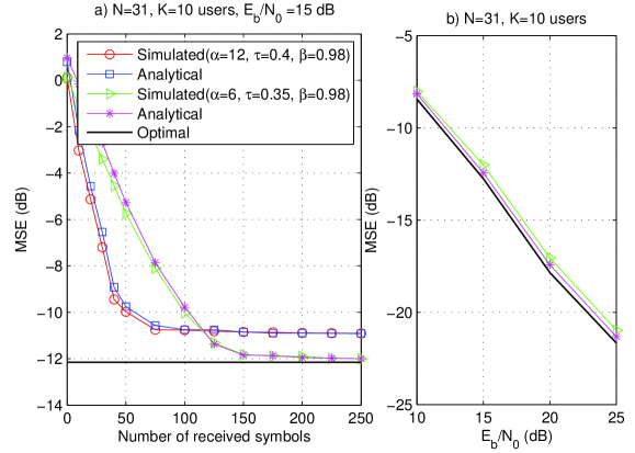
Refer to caption
Figure 2: MSE performance against a) the number of received symbols at Eb/N0=15โ€‹dโ€‹Bsubscript๐ธ๐‘subscript๐‘015๐‘‘๐ตE_{b}/N_{0}=15dB and b) Eb/N0subscript๐ธ๐‘subscript๐‘0E_{b}/N_{0} (dB).

The tracking analysis of the proposed SM-CCM-SG algorithm in a time-varying multipath fading channel is discussed next. We consider the same scenario as before except for the fact that the channel is now time-varying and the analytical results of the tracking analysis in (80) are employed. We consider a Jakesโ€™ model with a typical normalized fading rate fdโ€‹Tsubscript๐‘“๐‘‘๐‘‡f_{d}T. We compute Trโ€‹(๐‘ธ)Tr๐‘ธ{\rm Tr}({\boldsymbol{Q}}) with the aid of J0โ€‹(2โ€‹ฯ€โ€‹fdโ€‹T)subscript๐ฝ02๐œ‹subscript๐‘“๐‘‘๐‘‡J_{0}(2\pi f_{d}T) [45], which is the autocorrelation function of the Jakesโ€™ model and where J0subscript๐ฝ0J_{0} is the zero-order Bessel function of the first kind. A comparison of the curves obtained by simulations and by the analytical formulas is shown in Fig. 3. Similarly to the case of fixed channels, the analytical and simulated curves agree and show the validity of the proposed formulas. Nevertheless, the curves indicate a higher misadjustment as compared to the curves in Fig. 2 due to the time-varying process and extra effort of the adaptive filters to track the channel variations.
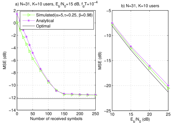
Refer to caption
Figure 3: MSE performance against a) the number of received symbols at Eb/N0=15โ€‹dโ€‹Bsubscript๐ธ๐‘subscript๐‘015๐‘‘๐ตE_{b}/N_{0}=15dB and b) Eb/N0subscript๐ธ๐‘subscript๐‘0E_{b}/N_{0} (dB).

VI-B Interference Power and Channel Estimation
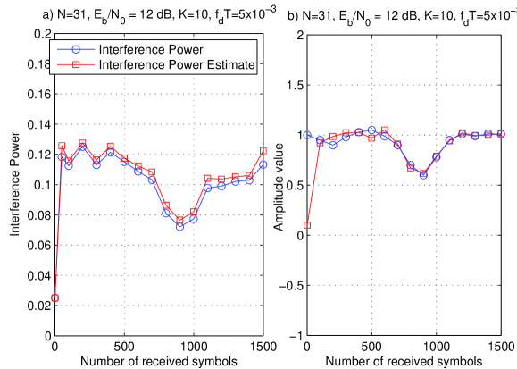
Refer to caption
Figure 4: Performance of the a) interference power estimation and tracking and b) amplitude estimation algorithms at Eb/N0=12โ€‹dโ€‹Bsubscript๐ธ๐‘subscript๐‘012๐‘‘๐ตE_{b}/N_{0}=12dB.

At this point, we wish to evaluate the effectiveness of the proposed algorithms for estimating and tracking the interference power and the amplitude. To this end, we have carried out an experiment, depicted in Fig. 4, where the proposed algorithm estimates of the MAI and ISI powers and the amplitude of the desired user are compared to the actual interference power and amplitude. The results show that the proposed algorithms are very effective for estimating and tracking the interference power in dynamic environments, as depicted in Fig. 4.

We assess the proposed channel estimation (CE) algorithm, called SM-CCM-CE, with the time-varying bounds PDB and PIDB, and also with a fixed bound, and compare them to the CMV-based method (CMV-CE) reported in [42] and the subspace algorithm of [43] in terms of the MSE between the actual and the estimated channels using the following dynamic scenario. The system has initially 101010 users, the power distribution among the interferers follows a log-normal distribution with associated standard deviation of 333 dB. After 150015001500 symbols, 666 additional users enter the system and the power distribution among interferers is loosen to 666 dB. The results, shown in Fig 5, reveal that the proposed SM-CCM-CE algorithm outperforms the CMV-CE technique reported in [42] because SM-CCM-CE uses a variable forgetting factor. The proposed SM-CCM is also computationally simpler than CMV-CE due to the sparse updates, whereas it is substantially less complex than the subspace method of [43]. This is because the SM-CCM-CE needs to compute the principal eigenvector of the Lpร—Lpsubscript๐ฟ๐‘subscript๐ฟ๐‘L_{p}\times L_{p} matrix ๐‘ชkโ€‹๐‘น^kโˆ’1โ€‹[i]โ€‹๐‘ชksubscript๐‘ช๐‘˜superscriptsubscript^๐‘น๐‘˜1delimited-[]๐‘–subscript๐‘ช๐‘˜{\boldsymbol{C}}_{k}\hat{\boldsymbol{R}}_{k}^{-1}[i]{\boldsymbol{C}}_{k}, while the subspace technique in [43] requires the principal eigenvector of the Mร—M๐‘€๐‘€M\times M matrix ๐‘น^โˆ’1โ€‹[i]superscript^๐‘น1delimited-[]๐‘–\hat{\boldsymbol{R}}^{-1}[i]. Since Lpโ‰ชMmuch-less-thansubscript๐ฟ๐‘๐‘€L_{p}\ll M in most practical scenarios SM-CCM-CE is typically considerably simpler than the subspace method.
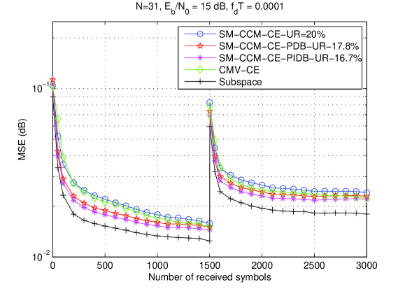
Refer to caption
Figure 5: MSE performance of channel estimation versus number of received symbols in a dynamic scenario where receivers operate at Sโ€‹Nโ€‹R=Eb/N0=15๐‘†๐‘๐‘…subscript๐ธ๐‘subscript๐‘015SNR=E_{b}/N_{0}=15 dB for the desired user.

VI-C BER Performance

The SM-CCM algorithms are assessed in a non-stationary environment where users enter and exit the system, as depicted in Figs. 6 and 7. The system starts with 222 interferers with 777 dB above the desired userโ€™s power level and 555 interferers with the same power level of the desired one, which corresponds to the signal-to-noise ratio Eb/N0=15subscript๐ธ๐‘subscript๐‘015E_{b}/N_{0}=15 dB. At 100010001000 symbols, 222 interferers with 101010 dB above the desired signal power level and 111 with the same power level enter the system, whereas 111 interferer with 777 dB above the desired signal power level leaves it. At 200020002000 symbols, 111 interferer with 101010 dB above, and 555 interferers with the same power level of the desired signal exit the system, while 111 interferer with 151515 dB above the desired user enters the system. The results for 100100100 runs show that the proposed SM-CCM-RLS algorithm achieves the best performance, followed by the proposed SM-CMV-RLS recursion, the CCM-SG and the CMV-SG methods. In summary the SM-CCM algorithms outperform the SM-CMV techniques in all scenarios and the SM-CCM-RLS algorithm is the best among the analyzed algorithms.

In a near-far scenario the eigenvalue spread of the covariance matrix of the received vector ๐’“โ€‹[i]๐’“delimited-[]๐‘–{\boldsymbol{r}}[i] is large, affecting the convergence performance of the SG algorithms with fixed step size and making it very difficult to compute a pre-determined value [2] for the step size. In this case, the SM-CCM algorithms are able to deal with near-far situations since they adopt variable step size or variable forgetting factor mechanisms, ensuring good tracking performance in dynamic scenarios and an improved performance over the existing CCM-type algorithms. In addition, due to their data-selective update feature the SM algorithms can save significant computational resources as they only require parameter updates for about 20%percent2020\% of the time for the SG-type recursions and around 12%percent1212\% for the RLS-based techniques.

Refer to caption
Figure 6: BER performance of the algorithms versus number of symbols for a non-stationary scenario. The parameters are ฮณ=1.3๐›พ1.3\gamma=1.3 for the SM-CMV, ฮณ=0.65๐›พ0.65\gamma=0.65 for the SM-CCM.
Refer to caption
Figure 7: BER performance of the algorithms versus number of symbols for a non-stationary scenario. The parameters are ฮณ=1.3๐›พ1.3\gamma=1.3 for the SM-CMV, ฮณ=0.65๐›พ0.65\gamma=0.65 for the SM-CCM.

The same scenario illustrated in Fig. 6 is considered for the SM-CCM algorithms with time-varying error bounds, as shown in Figs. 8 and 9. The results indicate that the proposed time-varying bounds are capable of improving the performance of SM algorithms, while further reducing the number of updates. The RLS-type algorithms outperform the SG-based techniques as expected and have lower Uโ€‹R๐‘ˆ๐‘…UR. Moreover, the algorithms with the PIDB approach achieve the best performance, followed by the algorithms with the PDB method and the SM recursions with fixed bounds. With respect to the Uโ€‹R๐‘ˆ๐‘…UR, the PIDB technique results in the smallest number of updates, followed by the PDB approach and the fixed bound.
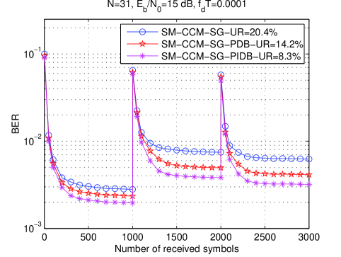
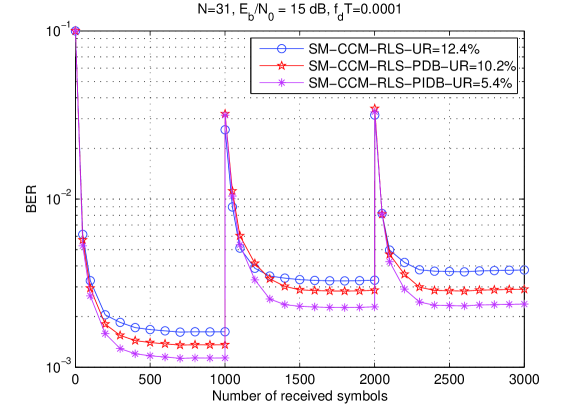
Refer to caption
Figure 8: BER performance of the SG algorithms versus number of symbols for a non-stationary scenario with time-varying bounds. The parameters are ฮฑ=8๐›ผ8\alpha=8, ฯ„=0.35๐œ0.35\tau=0.35 and ฮฒ=0.95๐›ฝ0.95\beta=0.95 for the time-varying bounds.
Refer to caption
Figure 9: BER performance of the RLS algorithms versus number of symbols for a non-stationary scenario with time-varying bounds. The parameters are ฮฑ=8๐›ผ8\alpha=8, ฯ„=0.35๐œ0.35\tau=0.35 and ฮฒ=0.95๐›ฝ0.95\beta=0.95 for the time-varying bounds.

The BER performance versus Eb/N0subscript๐ธ๐‘subscript๐‘0E_{b}/N_{0} and number of users is shown in Fig. 10. We consider data packets of P=1500๐‘ƒ1500P=1500 symbols and compare the proposed SM-CCM-RLS algorithm with a fixed bound, with the PIDB mechanism, the training-based BEACON algorithm with the PIDB mechanism [22] and the linear MMSE receiver that assumes perfect knowledge of the channels and the noise variance. We have measured the BER after 200200200 independent transmissions and the BEACON algorithm [7],[22] is trained with 200200200 symbols and is then switched to decision-directed mode. The curves illustrate that the proposed blind SM-CCM-RLS algorithm can approach the performance of the supervised BEACON algorithm and that of the linear MMSE receiver.
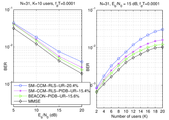
Refer to caption
Figure 10: BER performance versus (a) Eb/N0subscript๐ธ๐‘subscript๐‘0E_{b}/N_{0} with K=10๐พ10K=10 users and (b) number of users (K) at Eb/N0=15subscript๐ธ๐‘subscript๐‘015E_{b}/N_{0}=15 dB .

VII Conclusions

We have proposed SM-CCM adaptive algorithms for interference suppression in DS-CDMA systems. We have analyzed the optimization problem that gives rise to the SM-CCM algorithms and devised analytical expressions to predict their MSE performance with a good accuracy. The proposed SM-CCM algorithms are equipped with variable step sizes and forgetting factors and are only updated for a small fraction of time without incurring any performance degradation. A blind framework for SM estimation that takes into account parameter estimation dependency and MAI and ISI for multiuser communications has also been introduced to provide a time-varying bound that is robust against channel and SNR variations. Simulations have shown that the proposed SM-CCM algorithms outperform previously reported blind techniques for several scenarios.

Acknowledgement

The second author is grateful for the financial support provided by CNPq, a Brazilian research council, and FAPERJ, a Rio de Janeiro state research funding agency.

References

  • [1]
  • [2] P. S. R. Diniz, Adaptive Filtering: Algorithms and Practical Implementations, 2nd edition, Kluwer Academic Publishers, Boston, MA, 2002.
  • [3] S. Gollamudi, S. Nagaraj, S. Kapoor and Y. F. Huang, โ€œSet-Membership Filtering and a Set-Membership Normalized LMS Algorithm with an Adaptive Step Sizeโ€, IEEE Sig. Proc. Letters, vol. 5, No. 5, May 1998.
  • [4] S. Werner and P. S. R. Diniz, โ€œSet-membership affine projection algorithmโ€, IEEE Sig. Proc. Letters, vol 8., no. 8, August 2001.
  • [5] P. S. R. Diniz and S. Werner, โ€œSet-Membership Binormalized Data Re-using LMS Algorithms,โ€ IEEE Trans. Sig. Proc., vol. 51, no. 1, pp. 124-134, January 2003.
  • [6] S. Gollamudi, S. Kapoor, S. Nagaraj and Y. F. Huang, โ€œSet-Membership Adaptive Equalization and an Updator-Shared Implementation for Multiple Channel Communication Systemsโ€, IEEE Transactions on Signal Processing, vol. 46, no. 9, pp. 2372-2385, September 1998.
  • [7] S. Nagaraj, S. Gollamudi, S. Kapoor and Y. F. Huang, โ€œBEACON: an adaptive set-membership filtering technique with sparse updatesโ€, IEEE Transactions on Signal Processing, vol. 47, no. 11, November 1999.
  • [8] S. Nagaraj, S. Gollamudi, S. Kapoor, Y. F. Huang and J. R. Deller Jr., โ€œAdaptive Interference Suppression for CDMA Systems with a Worst-Case Error Criterion,โ€ IEEE Transactions on Signal Processing, vol. 48, No. 1, January 2000.
  • [9] S. Gollamudi, S. Nagaraj, and Y. F. Huang, โ€œBlind Equalization with a Deterministic Constant Modulus Cost - A Set-Membership Filtering Approachโ€, Proc. IEEE ICASSP, 2000.
  • [10] I. Akyildiz, W. Su, Y. Sankarasubramaniam, and E. Cayirci, โ€A survey on sensor networks,โ€ IEEE Communications Magazine, vol. 40, Issue 8, August, 2002, pp. 102-114.
  • [11] T. Wang, R. C. de Lamare, and P. D. Mitchell, โ€Low-Complexity Set-Membership Channel Estimation for Cooperative Wireless Sensor Networks,โ€ IEEE Transactions on Vehicular Technology, vol.60, no.6, pp.2594-2607, July 2011.
  • [12] D. Maksarov and J. P. Norton, โ€œTuning of noise bounds in parameter set estimation,โ€ in Proceedings of International Conference on Identification in Engineering Systems, Swansea, UK, 27-29, March 1996, pp. 584-593.
  • [13] S. Gazor and K. Shahtalebi, โ€œA New NLMS Algorithm for Slow Noise Magnitude Variationโ€, IEEE Signal Processing Letters, vol. 9, no. 11, November 2002.
  • [14] L. Guo and Y. F. Huang, โ€œSet-Membership Adaptive Filtering with Parameter-Dependent Error Bound Tuning,โ€ IEEE Proc. Int. Conf. Acoust. Speech and Sig. Proc., 2005.
  • [15] L. Guo and Y. F. Huang, โ€œFrequency-Domain Set-Membership Filtering and Its Applicationsโ€, IEEE Transactions on Signal Processing, Vol. 55, No. 4, April 2007, pp. 1326-1338.
  • [16] M. Z. A. Bhotto, and A. Antoniou, โ€œRobust Set-Membership Affine-Projection Adaptive-Filtering Algorithmโ€, IEEE Transactions on Signal Processing, vol. 60 , no. 1, January 2012 , pp. 73 - 81.
  • [17] T. M. Lin, M. Nayeri and J. R. Deller, Jr., โ€œConsistently Convergent OBE Algorithm with Automatic Selection of Error Bounds,โ€ International Journal of Adaptive Control and Signal Processing, vol. 12, pp. 302-324, June 1998.
  • [18] J. R. Deller, S. Gollamudi, S. Nagaraj, and Y. F. Huang, โ€œConvergence analysis of the QUASI-OBE algorithm and the performance implications,โ€ in Proc. IFAC Int. Symp. Syst. Ident., vol. 3, Santa Barbara, CA, June 2000, pp. 875-880.
  • [19] S. Dasgupta and Y. F. Huang, โ€œAsymptotically convergent modified recursive least-squares with data dependent updating and forgetting factor for systems with bounded noise,โ€ IEEE Trans. Inform. Theory, vol. IT-33, pp. 383โ€“392, 1987.
  • [20] J. R. Deller, M. Nayeri, and M. Liu, โ€œUnifying the landmark developments in optimal bounding ellipsoid identification,โ€ Int. J. Adap. Contr. Signal Process., vol. 8, pp. 43โ€“60, 1994.
  • [21] D. Joachim, J. R. Deller, and M. Nayeri, โ€œMultiweight optimization in OBE algorithms for improved tracking and adaptive identification,โ€ in Proc. IEEE Int. Acoust., Speech Signal Process., vol. 4, Seattle, WA, May 1998, pp. 2201-2204.
  • [22] R. C. de Lamare and P. S. R. Diniz, โ€œSet-Membership Adaptive Algorithms based on Time-Varying Error Bounds for CDMA Interference Suppressionโ€, IEEE Transactions on Vehicular Technology, vol. 58, no. 2, February 2009 , pp. 644 - 654.
  • [23] R. C. de Lamare and P. S. R. Diniz, โ€Blind constrained set-membership algorithms with time varying bounds for CDMA Interference Suppressionโ€, in Proc. IEEE International Conference on Acoustics, Speech and Signal Processing, May 2006.
  • [24] J.C. Liberti and T. S. Rappaport, Smart Antennas for Wireless Communications: IS-95 and Third Generation CDMA Applications, Prentice Hall: Upper Saddle River, New Jersey, 1999.
  • [25] M. Honig, U. Madhow and S. Verdu, โ€œBlind adaptive multiuser detection,โ€ IEEE Trans. Inf. Theory, vol. 41, pp. 944-960, July 1995.
  • [26] R. C. de Lamare and R. Sampaio-Neto, โ€œAdaptive Reduced-Rank Processing Based on Joint and Iterative Interpolation, Decimation, and Filtering,โ€ IEEE Transactions on Signal Processing, vol. 57, no. 7, July 2009, pp. 2503 - 2514.
  • [27] Z. Xu and M.K. Tsatsanis, โ€œBlind adaptive algorithms for minimum variance CDMA receivers,โ€ IEEE Trans. Communications, vol. 49, No. 1, January 2001.
  • [28] R. C. de Lamare and R. Sampaio-Neto, โ€œLow-Complexity Variable Step-Size Mechanisms for Stochastic Gradient Algorithms in Minimum Variance CDMA Receiversโ€, IEEE Trans. Signal Processing, vol. 54, pp. 2302 - 2317, June 2006.
  • [29] R. C. de Lamare, โ€œAdaptive Reduced-Rank LCMV Beamforming Algorithms Based on Joint Iterative Optimisation of Filtersโ€, Electronics Letters, vol. 44, no. 9, 2008.
  • [30] R. Fa, R. C. de Lamare and L. Wang, โ€œReduced-rank STAP schemes for airborne radar based on switched joint interpolation, decimation and filtering algorithmโ€, IEEE Trans. Sig. Proc., 2010, vol. 58, no. 8, pp.4182-4194.
  • [31] J. Miguez and L. Castedo, โ€œA linearly constrained constant modulus approach to blind adaptive multiuser interference suppression,โ€ IEEE Communications Letters, vol. 2, pp. 217-219, August 1998.
  • [32] C. Xu, G. Feng and K. S. Kwak, โ€œA Modified Constrained Constant Modulus Approach to Blind Adaptive Multiuser Detection,โ€ IEEE Trans. Communications, vol. 49, No. 9, 2001.
  • [33] Z. Xu and P. Liu, โ€œCode-Constrained Blind Detection of CDMA Signals in Multipath Channels,โ€ IEEE Sig. Proc. Letters, vol. 9, No. 12, December 2002.
  • [34] R. C. de Lamare and R. Sampaio Neto, โ€Blind Adaptive Code-Constrained Constant Modulus Algorithms for CDMA Interference Suppression in Multipath Channelsโ€, IEEE Communications Letters, vol 9. no. 4, April, 2005.
  • [35] R. C. de Lamare, M. Haardt and R. Sampaio-Neto, โ€œBlind Adaptive Constrained Reduced-Rank Parameter Estimation based on Constant Modulus Design for CDMA Interference Suppression,โ€ IEEE Transactions on Signal Processing, vol. 56., no. 6, June 2008.
  • [36] Y. Cai and R. C. de Lamare, โ€œLow-Complexity Variable Step Size Mechanism for Code-Constrained Constant Modulus Stochastic Gradient Algorithms applied to CDMA Interference Suppressionโ€, IEEE Transactions on Signal Processing, vol. 57, No. 1, January 2009.
  • [37] R. C. de Lamare and R. Sampaio-Neto, โ€œBlind adaptive MIMO receivers for space-time block-coded DS-CDMA systems in multipath channels using the constant modulus criterion,โ€ IEEE Transactions on Communications, vol. 58, no. 1, January 2010, pp. 21-27.
  • [38] R.C. de Lamare, R. Sampaio-Neto and M. Haardt, โ€Blind Adaptive Constrained Constant-Modulus Reduced-Rank Interference Suppression Algorithms Based on Interpolation and Switched Decimation,โ€ IEEE Trans. on Signal Processing, vol.59, no.2, pp.681-695, Feb. 2011.
  • [39] J. Mai and A. H. Sayed,โ€œA feedback approach to the steady-state performance of fractionally spaced blind adaptive equalizers,โ€ IEEE Trans. Signal Process., vol. 48, no. 1, pp. 80โ€“91, Jan. 2000.
  • [40] N. R. Yousef and A. H. Sayed, โ€œA unified approach to the steady-state and tracking analyses of adaptive filters,โ€ IEEE Trans. Signal Process., vol. 49, no. 2, pp. 314โ€“324, Feb. 2001.
  • [41] J. Whitehead and F. Takawira, โ€œPerformance analysis of the linearly constrained constant modulus algorithm-based multiuser detector,โ€ IEEE Trans. Signal Process., vol. 53, no. 2, pp. 643โ€“653, Feb. 2005.
  • [42] X. G. Doukopoulos and G. V. Moustakides, โ€œAdaptive Power Techniques for Blind Channel Estimation in CDMA Systemsโ€, IEEE Trans. Signal Processing, vol. 53, No. 3, March, 2005.
  • [43] X. Wang and H. V. Poor, โ€œBlind multiuser detection: A subspace approach,โ€ IEEE Transactions on Information Theory, vol. 44, pp. 677-690, March 1998.
  • [44] D. P. Bertsekas, Nonlinear Programming, Athena Scientific, 2nd Ed., 1999.
  • [45] T. S. Rappaport, Wireless Communications, Prentice-Hall, Englewood Cliffs, NJ, 1996.