A control strategy algorithm for finite alternating transition systems

Abstract

Recently, there has been an increasing interest in the formal analysis and design of control systems. In this area, in order to reduce the complexity and scale of control systems, finite abstractions of control systems are introduced and explored. Amongst, Pola and Tabuada construct finite alternating transition systems as approximate finite abstractions for control systems with disturbance inputs [SIAM Journal on Control and Optimization, Vol. 48, 2009, 719-733]. Given linear temporal logical formulas as specifications, this paper provides a control strategy algorithm to find control strategies of Pola and Tabuada’s abstractions enforcing specifications.

1 Introduction

The formal analysis and design of control systems is one of recent trends in control theory. The formal analysis is concerned with verifying whether a control system satisfies a desired specification, while the purpose of the formal design is to construct a controller for control system so that it meets a given specification. Traditionally, stability and reachability are considered as specifications in the control-theoretic community [12, 13]. Recently, there has been an increasing interest in extending the formal analysis and design by considering more complex specifications [1, 4, 8, 9, 17, 18, 20, 27, 29]. In these work, temporal logic [1, 4, 8, 9, 17, 27], regular expressions [18], and transition systems [29] are used to describe specifications. Amongst, temporal logic, due to its resemblance to natural language and the existence of algorithms for model checking, is widely adopted for task specification and controller synthesis in control theory. For example, linear temporal logic (LTL) has been adopted to describe the desired properties of discrete-time linear systems [27] and continuous-time linear systems [17]. In addition, Computation Tree Logic (CTL)[4] and LTL[8, 9] are applied to express specifications in the area of mobile robotics.

The formal analysis and design of large-scale control systems is difficult because of the complexity and scale of systems. In order to reduce the complexity and scale, finite abstractions are extracted from these control systems [1, 27, 29]. Usually, finite abstractions and original systems share properties of interest and the analysis and design of finite abstractions is simpler than that of original control systems. Thus the analysis and design of control systems is often equivalently performed on the corresponding finite abstractions. So finite abstractions are extremely useful in the formal analysis and design.

Much work has been devoted to the construction of finite abstractions of control systems. For instance, Tabuada and Pappas identify critical properties of discrete-time linear systems ensuring the existence of finite abstractions [28]. Symbolic models of nonlinear control systems are constructed in [25, 30]. Finite abstractions of hybrid systems are studied in [2, 3, 14, 15, 21]. An excellent review of these work may be found in [1].

In the work mentioned above, researchers consider control systems without reference to disturbances. However, as pointed out by B C. Kuo in [19], all physical systems are subject to some types of extraneous disturbances or noise during operation. Recently, Pola and Tabuada extend the above work to control systems affected by disturbances [23, 24]. A mathematical structure called alternating transition system is presented as symbolic abstraction of control system with disturbance inputs [23, 24]. Under the assumption that control systems are bounded, such abstractions are finite.

In [9][27][29], usual transition systems are adopted as finite abstractions of control systems. Some approaches are presented to construct control strategies of these finite abstractions enforcing specifications. Further, based on such control strategies, controllers of original control systems are generated to meet specifications. So the construction of control strategies of finite abstractions is one of the important steps in the formal design of control systems. However, since Pola and Tabuada’s abstractions [23, 24] are modeled by alternating transition systems rather than usual transition systems, the approaches provided in [9][27][29] are not suitable for establishing control strategies for Pola and Tabuada’s abstractions. To overcome this defect, this paper will present a control strategy algorithm based on Kabanza et al.’s planning algorithm [16] to solve the following control problem: given a finite, non-blocking alternating transition system $T$ and a specification, how to find an initial state and a control strategy of $T$ enforcing the given specification? Clearly, this algorithm can be used to find control strategies for Pola and Tabuada’s finite abstractions.

The rest of this paper is organized as follows. In Section 2, we recall the notion of alternating transition system and present the control problem mentioned above in detail. Section 3 recalls some notions and results about Kabanza et al.’s planning algorithm. Based on their algorithm, Section 4 provides a control strategy algorithm. In Section 5, we explore the correctness and completeness of this algorithm. Finally, we conclude the paper with future work in Section 6. The appendix includes the proofs of some results of this paper.

2 Alternating transition system and control problem

Before recalling the notion of alternating transition system, we introduce some useful notations. The symbol $\mathbb{N}$ denotes the set of positive integers. For any set $A$, $A^{+}$ denotes the set of all non-empty finite strings over $A$, and $A^{\omega}$ represents the set of infinite strings over $A$. Usually, we put $A^{\infty}=A^{+}\cup A^{\omega}$. We use $s_{A}$, $\sigma_{A}$ and $\alpha_{A}$ to denote the elements of $A^{+}$, $A^{\omega}$ and $A^{\infty}$, respectively. If $A$ is known from the context, we will omit the subscript in $s_{A}$, $\sigma_{A}$ and $\alpha_{A}$. For any $s\in A^{+}$, $s[i]$ and $s[end]$ mean the $i$-th element and the last element of $s$, respectively. Given $i\leq j$, $s[i,j]$, $s[i,end]$ and $\sigma[i,\infty]$ represent $s[i]s[i+1]\cdots s[j]$, $s[i]s[i+1]\cdots s[end]$ and $\sigma[i]\sigma[i+1]\cdots$, respectively. As usual, $|s|$ means the length of $s$. For any $\sigma\in A^{\omega}$, $|\sigma|$ is set to be $\infty$.

Pola and Tabuada provide finite abstractions for control systems with disturbance inputs. For these control systems, the inputs consist of control and disturbance inputs, where the former are controllable and the latter are not. Usual transition system can not capture the different roles played by these two kinds of inputs. To overcome this obstacle, Pola and Tabuada adopt alternating transition systems as models of these control systems and their abstract systems [23, 24].

Definition 1.

An alternating transition system is a tuple:

$T=(Q,A,B,\longrightarrow,O,H)$,

consisting of

$\bullet$ a set of states $Q$;

$\bullet$ a set of control labels $A$;

$\bullet$ a set of disturbance labels $B$;

$\bullet$ a transition relation $\rightarrow\subseteq Q\times A\times B\times Q$;

$\bullet$ an observation set $O$;

$\bullet$ an observation function $H:Q\rightarrow O$.

An alternating transition system is said to be

$\bullet$ finite if $Q$, $A$ and $B$ are finite;

$\bullet$ non-blocking if $\{q^{\prime}:q\xrightarrow{a,b}q^{\prime}\}\not=\emptyset$ for any $q\in Q$, $a\in A$ and $b\in B$.

An infinite sequence $\sigma\in Q^{\omega}$ is said to be a trajectory of $T$ if and only if for all $i\in\mathbb{N}$, $\sigma[i]\xrightarrow{a_{i},b_{i}}\sigma[i+1]$ for some $a_{i}\in A$ and $b_{i}\in B$.

In the above definition, a transition label is a pair $<a,b>$, where the former is used to denote control input and the latter represents disturbance input. Pola and Tabuada construct non-blocking alternating transition systems as abstractions of control systems with disturbance inputs [23, 24]. Under the assumption that control systems are bounded, their abstractions are finite. The related notions and results can be found in [23, 24].

This paper aims to provide an approach to obtain control strategies of Pola and Tabuada’s finite abstractions to meet specifications. Formally, we will solve the following control problem:

Problem 1.

Given a finite, non-blocking alternating transition system $T$ and a specification, how to find an initial state and a control strategy of $T$ enforcing the given specification?

In this paper, the specifications mentioned above will be described by the linear temporal logic LTL_-X [7]. The LTL_-X formulae have been used to specify the desired properties of control system and its abstraction in [17]. We recall this logic below.

Definition 2.

[7, 17] Let $\mathbb{P}$ be a finite set of atomic propositions. The linear temporal logic LTL${}_{-X}(\mathbb{P})$ formula over $\mathbb{P}$ is inductively defined as:

$\varphi::=p|\neg\varphi|\varphi_{1}\wedge\varphi_{2}|\varphi_{1}\mathbf{U}\varphi_{2}$

where $p\in\mathbb{P}$.

The operator $\mathbf{U}$ is read as “until” and the formula $\varphi_{1}\mathbf{U}\varphi_{2}$ specifies that $\varphi_{1}$ must hold until $\varphi_{2}$ holds. The semantics of LTL${}_{-X}(\mathbb{P})$ formulae are defined below.

Definition 3.

Let $\sigma_{\mathbb{P}}$ be any infinite word over $2^{\mathbb{P}}$ (i.e.,$\sigma_{\mathbb{P}}\in(2^{\mathbb{P}})^{\omega}$). The satisfaction of LTL${}_{-X}(\mathbb{P})$ formula $\varphi$ at position $i\in\mathbb{N}$ of the word $\sigma_{\mathbb{P}}$, denoted by $\sigma_{\mathbb{P}}[i]\models\varphi$, is defined inductively as follows:

(1) $\sigma_{\mathbb{P}}[i]\models p$ iff $p\in\sigma_{\mathbb{P}}[i]$;

(2) $\sigma_{\mathbb{P}}[i]\models\neg\varphi$ iff $\sigma_{\mathbb{P}}[i]\models\varphi$ does not hold;

(3) $\sigma_{\mathbb{P}}[i]\models\varphi_{1}\wedge\varphi_{2}$ iff $\sigma_{\mathbb{P}}[i]\models\varphi_{1}$ and $\sigma_{\mathbb{P}}[i]\models\varphi_{2}$;

(4) $\sigma_{\mathbb{P}}[i]\models\varphi_{1}\mathbf{U}\varphi_{2}$ iff there exists $j\geq i$ such that $\sigma_{\mathbb{P}}[j]\models\varphi_{2}$ and for all $k\in\mathbb{N}$ with $i\leq k<j$, we have $\sigma_{\mathbb{P}}[k]\models\varphi_{1}$.

A word $\sigma_{\mathbb{P}}$ satisfies an LTL${}_{-X}(\mathbb{P})$ formula $\varphi$, written as $\sigma_{\mathbb{P}}\models\varphi$, if and only if $\sigma_{\mathbb{P}}[1]\models\varphi$.

Definition 4.

Let $T=(Q,A,B,\longrightarrow,O,H)$ be a finite, non-blocking alternating transition system, $\mathbb{P}$ a finite set of atomic propositions and let $\prod:Q\rightarrow 2^{\mathbb{P}}$ be a valuation function. For any LTL${}_{-X}(\mathbb{P})$ formula $\phi$, an infinite sequence $\sigma\in Q^{\omega}$ is said to satisfy $\phi$ w.r.t $\prod$, written as $\sigma\models_{\prod}\phi$, if and only if $\prod(\sigma)\models\phi$, where $\prod(\sigma)\triangleq\prod(\sigma[1])\prod(\sigma[2])\cdots$.

If the valuation function $\prod$ is known from the context, we often omit the subscript in $\models_{\prod}$.

3 Kabanza et al.’s algorithm

To solve Problem 1, we will provide a control strategy algorithm based on Kabanza et al.’s planning algorithm. This section recalls some notions and results about Kabanza et al.’s algorithm. More details can be found in [16].

Kabanza et al. develop their work in the framework of reactive agent. Given a finite set $Q$ of world states, a reactive agent is described as a pair $(q_{0},succ)$, where $q_{0}\in Q$ is an initial world state and $succ$ is a transition function. For any world state $q\in Q$, $succ(q)$ returns a list $((a_{1},d_{1},W_{1}),\cdots,(a_{n},d_{n},W_{n}))$, where $a_{i}$ is an action that is executable in $q$, $d_{i}$ is a strictly positive real number denoting the duration of $a_{i}$ in $q$, and $W_{i}\subseteq Q$ is the set of nondeterministic successors resulting from the execution of $a_{i}$ in $q$. As usual, if $q^{\prime}\in W_{i}$ for some $i\leq n$, then we denote by $q\xrightarrow{a_{i}}q^{\prime}$ that $q^{\prime}$ is a successor of $q$ resulting from the execution of $a_{i}$ in $q$.

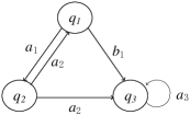
Fig. 1: Reactive Agent

Example 3.1.

Fig 1 illustrates the reactive agent ($q_{1},succ$) , where $succ(q_{1})=((a_{1},1,\{q_{2}\}),(b_{1},1,\{q_{3}\}))$, $succ(q_{2})=((a_{2},1,\{q_{1},q_{3}\}))$, and $succ(q_{3})=((a_{3},1,\{q_{3}\}))$. Since the durations of all actions are $1$, we do not indicate them in this figure.

Definition 5.

[16] A reactive plan is represented by a set of situation control rules (SCRs), where an SCR is a tuple of the form $(n,q,a,N)$ such that:

$\bullet$ $n$ is a number denoting a plan state;

$\bullet$ $q$ is the world state labeling the plan state $n$ and describing the situation when this SCR is applied;

$\bullet$ $a$ is the action to be executed in plan state $n$; and

$\bullet$ $N$ is a set of integers denoting plan states that are nondeterministic successors of $n$ when $a$ is executed .

In the above definition, two kinds of states are referred to: world states and plan states. Each plan state is labeled by a world state and different plan states may be labeled by the same world state. Roughly speaking, these plan states labeled by the same world state $q$ may denote different executive pathes along which the world state $q$ is reached. So, since the actions to be executed in different plan states may not be identical, the choice of the actions in the world state $q$ can be history dependent. That is, when $q$ is reached along different pathes, the actions to be executed in $q$ may be different. Before providing an example to illustrate the above argument, we describe the execution of a reactive plan as follows.

We start the execution of a reactive plan by fetching the SCR corresponding to the initial world state. By convention, this is always the SCR with plan state 1. The corresponding world state describes the current situation before the agent executes any action. At any time, given the current SCR $(n,q,a,N)$, the action $a$ is executed and the SCR matching the resulting situation is determined from the successor plan states in $N$ by getting an SCR $(n^{\prime},q^{\prime},a^{\prime},N^{\prime})$ such that $n^{\prime}\in N$. In this case, the current situation is $q^{\prime}$ and then $a^{\prime}$ is executed.

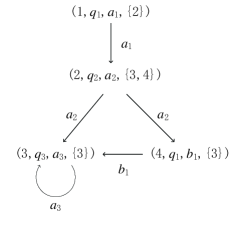
Fig. 2: Executing Reactive Plan

Example 3.2.

Consider the reactive agent provided in Example 3.1. Given a reactive plan

$RP=\{(1,q_{1},a_{1},\{2\}),(2,q_{2},a_{2},\{3,4\}),(3,q_{3},a_{3},\{3\}),(4,q_{1},b_{1},\{3\})\}$,

its execution is illustrated by Fig 2.

In this reactive plan, both plan states 1 and 4 are labeled by world state $q_{1}$. Plan state 1 represents that $q_{1}$ is the initial state, while plan state 4 means that $q_{1}$ is reached from $q_{2}$ by executing $a_{2}$. Then it is easy to see that the actions to be executed in $q_{1}$ may be different when the pathes along which $q_{1}$ is reached is different.

The trajectory generated by reactive plan is defined as follows.

Definition 6.

[16] Let $(q_{1},succ)$ be a reactive agent and let $RP=\{((1,q_{1},a_{1},N_{1}),\\ (2,q_{2},a_{2},N_{2}),\cdots(k,q_{k},a_{k},N_{k}))\}$ be a reactive plan of $(q_{1},succ)$. An infinite sequence $\sigma$ of world states is said to be a trajectory generated by the reactive plan $RP$ if and only if there exists an infinite sequence $\sigma_{N}=i_{1}i_{2}\cdots\in\{1,2,\cdots,k\}^{\omega}$ such that $\sigma_{N}[1]=1$ and for all $j\in\mathbb{N}$, $i_{j+1}\in N_{i_{j}}$ and $q_{i_{j}}=\sigma[j]$.

Example 3.3.

Consider the reactive agent and the reactive plan $RP$ in Example 3.1 and 3.2, respectively. Let $\sigma_{1}=q_{1}q_{2}q_{3}^{\omega}$ and $\sigma_{2}=q_{1}q_{2}q_{1}q_{3}^{\omega}$. It is easy to check that $\sigma_{1}$ and $\sigma_{2}$ are exactly trajectories generated by this reactive plan.

Definition 7.

Let $\mathbb{P}$ be a finite set of atomic propositions and let $\prod$ be a valuation function that assigns each world state $q$ a set $\prod(q)\subseteq\mathbb{P}$. For any LTL${}_{-X}(\mathbb{P})$ formula $\phi$, a reactive plan is said to satisfy $\phi$ w.r.t. $\prod$ if and only if all trajectories generated by this reactive plan satisfy $\phi$ w.r.t. $\prod$ and there exists at least one trajectory generated by this reactive plan.

Example 3.4.

Consider the reactive agent and the reactive plan $RP$ in Example 3.1 and 3.2, respectively. Let $\mathbb{P}=\{p_{1},p_{2},p_{3}\}$ and let $\prod:\{q_{1},q_{2},q_{3}\}\rightarrow 2^{\mathbb{P}}$ be a valuation function defined as: $\prod(q_{1})=\{p_{1},p_{2}\}$, $\prod(q_{2})=\{p_{2},p_{3}\}$ and $\prod(q_{3})=\{p_{1},p_{3}\}$. It is easy to check that the reactive plan $RP$ satisfies $p_{2}\mathbf{U}p_{3}$ w.r.t. $\prod$.

In [16], Kabanza et al. use Metric Temporal Logic (MTL) to specify the desired behaviors of reactive agent. Given a finite set $\mathbb{P}$ of atomic propositions, MTL($\mathbb{P}$) formulae are defined as:

$$\varphi::=p|\neg\varphi|\varphi_{1}\wedge\varphi_{2}|X_{\sim t}\varphi|\Box_{\sim t}\varphi|\varphi_{1}\mathbf{U}_{\sim t}\varphi_{2}$$

where $p\in\mathbb{P}$ is atomic proposition, $X_{\sim t}$, $\Box_{\sim t}$ and $\mathbf{U}_{\sim t}$ are called the next, always and until operators, respectively, $\sim$ denotes either $\leq$, $<$, $\geq$ or $>$, and $t$ is a non-negative real. Intuitively, if a time constraint ”$\sim t$” is associated to a modal operator, then the modal formula connected by this modal operator must hold within a time period satisfying the relation “$\sim t$”. For example, $\varphi_{1}\mathbf{U}_{\geq t}\varphi_{2}$ means that $\varphi_{1}$ holds until $\varphi_{2}$ becomes true on the semi-open time interval $[t,\infty)$. So it is easy to see that $\mathbf{U}_{\geq 0}$ coincides with the usual $until$ operator $\mathbf{U}$. Thus linear temporal logic LTL_-X($\mathbb{P}$) can be viewed as a sublanguage of MTL($\mathbb{P}$).

Kabanza et al. also define the semantics of MTL$(\mathbb{P})$. A careful examination shows that, when we only consider LTL_-X$(\mathbb{P})$ formulas, Kabanza et al.’s definition is coincided with Definition 7. Since the remainder of this paper will mostly refer to LTL${}_{-X}(\mathbb{P})$ formulas, we do not recall the formal definition of the semantics of MTL($\mathbb{P})$. The interested reader may find it in Section 5.2 in [16].

Kabanza et al. provide an planning algorithm to construct a reactive plan satisfying an MTL($\mathbb{P}$) formula $\phi$ for the given reactive agent and valuation function $\prod$. The detailed algorithm may be found in [16]. The following result comes from Theorem 16 and the observation in Section 7.5 in [16].

Theorem 8.

[16] Kabanza et al. planning algorithm is correct and complete. In other words, given a reactive agent $(q_{0},succ)$, an MTL($\mathbb{P}$) formula $\phi$ and a valuation function $\prod$, if Kabanza et al.’s algorithm returns a reactive plan then this reactive plan satisfies $\phi$. Moreover, Kabanza et al.’s algorithm can find a reactive plan satisfying $\phi$ if such plan exists.

Immediately, we have the following corollary, which is trivial but useful.

Corollary 9.

Given a reactive agent $(q_{0},succ)$, an LTL_-X($\mathbb{P}$) formula $\phi$ and a valuation function $\prod$, if Kabanza et al.’s algorithm returns a reactive plan then this reactive plan satisfies $\phi$. Moreover, Kabanza et al.’s algorithm can find a reactive plan satisfying $\phi$ if such plan exists.

Proof.

Follows from Theorem 8 and the fact that linear temporal logic LTL_-X($\mathbb{P}$) can be viewed as a sublanguage of MTL($\mathbb{P}$).   ∎

4 Control strategy algorithm based on Kabanza et al.’s algorithm

The previous section has provided a brief overview about Kabanza et al.’s planning algorithm. This section will present a control strategy algorithm based on Kabanza et al.’s algorithm. Before providing this algorithm, we introduce the notion of control strategy.

Definition 10.

Let $T=(Q,A,B,\longrightarrow,O,H)$ be a finite, non-blocking alternating transition system. For any function $f:Q^{+}\rightarrow A$, we say $f$ is a control strategy of $T$. For any $q\in Q$ and $f:Q^{+}\rightarrow A$, the outcomes $Out^{n}_{T}(q,f)$ $(n\in\mathbb{N})$ and $Out_{T}(q,f)$ of $f$ from $q$ are defined as follows:

$$Out^{n}_{T}(q,f)=\{s\in Q^{n}: s[1]=q\ \mathrm{and}\ \forall 1\leq i<n\exists b_{i}\in B(s[i]\xrightarrow{f(s[1,i]),b_{i}}s[i+1])\},$$

$$Out_{T}(q,f)=\{\sigma\in Q^{\omega}: \sigma[1]=q\ \mathrm{and}\ \forall i\in\mathbb{N}\exists b_{i}\in B(\sigma[i]\xrightarrow{f(\sigma[1,i]),b_{i}}\sigma[i+1])\}.$$

Furthermore, we define $Out^{+}_{T}(q,f)$ and $Out^{\infty}_{T}(q,f)$ as: $Out^{+}_{T}(q,f)=\bigcup_{n\in\mathbb{N}}Out^{n}_{T}(q,f)$ and $Out^{\infty}_{T}(q,f)=Out^{+}_{T}(q,f)\cup Out_{T}(q,f)$.

If alternating transition system $T$ is known from the context, we often omit the subscripts in $Out^{n}_{T}(q,f)$, $Out_{T}(q,f)$, $Out^{+}_{T}(q,f)$, and $Out^{\infty}_{T}(q,f)$.

Given a finite, non-blocking alternating transition system $T$, an LTL${}_{-X}(\mathbb{P})$ formula $\phi$ and a valuation function $\prod$, we want to find an initial state $q$ and a control strategy $f$ of $T$ so that $\sigma\models\phi$ for all $\sigma\in Out(q,f)$. An algorithm, which is used to find such initial state and control strategy, is presented in Algorithm 1 below.

(1) input : $T$, $\phi$ and $\prod$, where $T=(Q,A,B,\longrightarrow,O,H)$

(2) Construct a transition function $succ_{T}$ from $T$

(3) for all $q_{0}\in Q$ do

(4)     Adopt Kabanza et al.’s algorithm to find a reactive plan $RP_{kab}$ of $(q_{0},succ_{T})$ enforcing $\phi$ w.r.t. $\prod$

(5)     if reactive plan $RP_{kab}$ is found then

(6)         $RP$=SimplyReactivePlan($RP_{kab}$)        /*See Algorithm 2 */

(7)         $f_{RP}$=FunctionStrategy($RP$)              /*See Algorithm 3 */

(8)        Return $q_{0}$ and $f_{RP}$

(9)     end if

(10) end for

(11) Return false

Algorithm 1 Control strategy algorithm

In Algorithm 1, steps (2), (6) and (7) are needed to be further refined. We illustrate them in turn.

Definition 11.

Let $T=(Q,A,B,\longrightarrow,O,H)$ be a finite, non-blocking alternating transition system and $A=\{a_{1},a_{2},\cdots,a_{k}\}$. The transition function $succ_{T}$ w.r.t $T$ is defined as: for any $q\in Q$, we set $succ_{T}(q)=((a_{1},1,W_{1}),(a_{2},1,W_{2}),\cdots,(a_{k},1,W_{k}))$, where $W_{i}\triangleq\{q^{\prime}\in Q:q\xrightarrow{a_{i},b}q^{\prime}\ \mathrm{for}\ \mathrm{some}\ b\in B\}$ for $i=1,2,\cdots k$.

By Definition 1, for any finite, non-blocking alternating transition system $T=\\ (Q,A,B,\longrightarrow,O,H)$, each set $W_{i}$ mentioned above is finite and non-empty. Thus for any $q\in Q$, $(q,succ_{T})$ is a reactive agent. Clearly, due to the finiteness of $Q$, $A$, $B$ and $\rightarrow$, the function $succ_{T}$ may be obtained using a simple algorithm. We leave it to interested reader. Before refining steps (6) and (7), we provide some notions and result below.

Definition 12.

Let $T=(Q,A,B,\longrightarrow,O,H)$ be a finite, non-blocking alternating transition system, $q\in Q$ and let $succ_{T}$ be the transition function w.r.t $T$. Then any reactive plan of $(q,succ_{T})$ is said to be a reactive plan of $T$.

Definition 13.

Let $RP=\{(1,q_{1},a_{1},N_{1}),(2,q_{2},a_{2},N_{2}),\cdots,(k,q_{k},a_{k},N_{k})\}$ be a reactive plan. For any finite sequence $s\in\{1,2,\cdots,k\}^{+}$, if $|s|>1$ and $s[i+1]\in N_{s[i]}$ for all $i<|s|$, then $s$ is said to be a finite path of $RP$. For any two pathes $s_{1}$ and $s_{2}$ of $RP$, if $s_{1}[1]=1$ and $s_{1}[end]=s_{2}[1]=s_{2}[end]$, then the pair $(s_{1},s_{2})$ is said to be a reachable cycle of $RP$.

The following result offers a sufficient and necessary condition for the existence of trajectory generated by reactive plan.

Lemma 14.

Let $RP=\{(1,q_{1},a_{1},N_{1}),(2,q_{2},a_{2},N_{2}),\cdots,(k,q_{k},a_{k},N_{k})\}$ be a reactive plan. There exists a trajectory generated by $RP$ if and only if there exists a reachable cycle $(s_{1},s_{2})$ of $RP$.

Proof.

(From Right to Left) Let $(s_{1},s_{2})$ be a reachable cycle of $RP$. By Definition 13, we have $|s_{2}|>1$. Then we set $\sigma_{N}=s_{1}\circ(s_{2}[2,end])^{\omega}$, where $(s_{2}[2,end])^{\omega}\triangleq s_{2}[2,end]\circ s_{2}[2,end]\circ\cdots$. Since $(s_{1},s_{2})$ is a reachable cycle of $RP$, it follows from Definition 13 that $\sigma_{N}[1]=1$ and $\sigma_{N}[i+1]\in N_{\sigma_{N}[i]}$ for all $i\in\mathbb{N}$. Then we define an infinite $\sigma\in\{q_{1},q_{2},\cdots,q_{k}\}^{\omega}$ as: $\sigma[i]=q_{\sigma_{N}[i]}$ for all $i\in\mathbb{N}$. Therefore, since $\sigma_{N}[1]=1$ and $\sigma_{N}[i+1]\in N_{\sigma_{N}[i]}$ for all $i\in\mathbb{N}$, by Definition 6, $\sigma$ is generated by $RP$.

(From Left to Right) Let $\sigma$ be a trajectory generated by $RP$. Then by Definition 6, there exists $\sigma_{N}\in\{1,2,\cdots,k\}^{\omega}$ such that $\sigma_{N}[1]=1$ and for all $i\in\mathbb{N}$, $\sigma[i]=q_{\sigma_{N}[i]}$ and $\sigma_{N}[i+1]\in N_{\sigma_{N}[i]}$. Since the plan state set $\{1,2,\cdots,k\}$ is finite, there exist $j,n\in\mathbb{N}$ such that $1<j<n$ and $\sigma_{N}[j]=\sigma_{N}[n]$. Further, by Definition 13, it is clear that $(\sigma_{N}[1,j],\sigma_{N}[j,n])$ is a reachable cycle of $RP$, as desired.   ∎

Now we refine steps (6) and (7). These two steps aim to get a control strategy from a reactive plan.

Step (6): In this step, given a reactive plan $RP$, we will simplify it in this way: for any $(i,q_{i},a_{i},N_{i})$ in $RP$, if there exist $j_{1},j_{2},\cdots,j_{m}\in N_{i}$ with $m>1$ and $q_{j_{1}}=q_{j_{n}}$ for all $n\leq m$, then we remain one of them and remove others from $N_{i}$. Thus for any $(i,q_{i},a_{i},N_{i})$ in the simplified reactive plan and for any world state $q$, there exists at most one plan state $j\in N_{i}$ with $q_{j}=q$. Formally, Step (6) is refined in Algorithm 2.

Suppose that $RP=\{(1,q_{1},a_{1},N_{1}),(2,q_{2},a_{2},N_{2}),\cdots,(k,q_{k},a_{k},N_{k})\}$

(1) SimplifyReactivePlan($RP$){

(2) $note=0$

(3) while $i\leq k$ and $note=0$ do

(4)    suffix=shortest_ path(i,i)

(5)    if suffix$\neq\emptyset$ then

(6)       prefix=shortest_ path(1,i)

(7)       if $prefix\neq\emptyset$ then

(8)           $note=1$;

(9)       end if

(10)    end if

(11) end while

(12) for all $(i,q_{i},a_{i},N_{i})\in RP$

(13)    for all $j_{1},j_{2},\cdots,j_{m}\in N_{i}$ with $m>1$ and $q_{j_{1}}=q_{j_{2}}=\cdots=q_{j_{m}}$

(14)       if for some $l\leq m$, there exists $n<|$prefix$|$ such that i=prefix[n] and $j_{l}$=prefix[n+1] then

(15)          $N_{i}=N_{i}-\{j_{1},\cdots,j_{l-1},j_{l+1},\cdots,j_{m}\}$ /$*$Remove $j_{1},\cdots,j_{l-1},j_{l+1},$ $\cdots,j_{m}$ from $N_{i}$ $*$/

(16)       else if for some $l\leq m$, there exists $n<|$suffix$|$ such that i=suffix[n] and $j_{l}$=suffix[n+1] then

(17)          $N_{i}=N_{i}-\{j_{1},\cdots,j_{l-1},j_{l+1},\cdots,j_{m}\}$ /$*$Remove $j_{1},\cdots,j_{l-1},j_{l+1},$ $\cdots,j_{m}$ from $N_{i}$ $*$/

(18)       else if

(19)          $N_{i}=N_{i}-\{j_{2},j_{3},\cdots,j_{m}\}$          /$*$Remove $j_{2},j_{3},\cdots,j_{m}$ from $N_{i}$ $*$/

(20)       end if

(21)    end for

(22) end for

(23) Return $RP$}

Algorithm 2 Simplifying reactive plan $RP$

In this algorithm, the lines (3)-(11) is used to find a reachable cycle (prefix,suffix). Amongst, we adopt DijKstra’s algorithm [5][6] to find the shortest pathes of $RP$ from $i$ to $i$ and from $1$ to $i$ (see lines (4) and (6)). By Lemma 14 and the completeness of DijKstra’s algorithm [5][6], prefix and suffix must can be found in this algorithm if the given reactive plan may generate trajectory.

Suppose that $RP$ may generate trajectory and the reachable cycle (prefix,suffix) has been found. The lines (12)-(22) aim to simplify the reactive plan $RP$ based prefix and suffix so that the simplified reactive plan may generate trajectory. Since prefix is the shortest path from 1 to prefix[end], it is clear that there do not exist $i,j<|$prefix$|$ such that $i\neq j$ and prefix[i]=prefix[j]. So, for the line (14) in Algorithm 2, there exists at most one natural number $l$ such that $l\leq m$, i=prefix[n] and $j_{l}$=prefix[n+1] for some $n<|$prefix$|$. Similar argument holds for the line (16). We provide a simple example below to illustrate Algorithm 2.

Example 4.1.

Consider the reactive plan $RP=\{(1,q_{1},a_{1},\{2\}),(2,q_{2},a_{2},\{1,4\}),\\ (3,q_{3},a_{3},\{1\}),(4,q_{1},a_{4},\{3\})\}$. We adopt Algorithm 2 to simplify $RP$. It is easy to check that both suffix and prefix found in this algorithm are “$121$”. For the SCR $(2,q_{2},a_{2},\{1,4\})\in RP$, since both plan states $1$ and 4 are labeled by $q_{1}$ and $pre\!fix=121$, plan state 4 is removed from $\{1,4\}$. One may easily examine that the simplified reactive plan is $\{(1,q_{1},a_{1},\{2\}),(2,q_{2},a_{2},\{1\}),(3,q_{3},a_{3},\{1\}),(4,q_{1},a_{4},\{3\})\}$.

In the above example, for the plan states 3 and 4 in the simplified reactive plan, there does not exist path from plan state $1$ to these states, although such pathes exist for the original reactive plan. Thus a natural question arises: whether the simplification provided in Algorithm 2 may result in that the simplified reactive plan can not generate trajectory although the original reactive plan can do so. The following result reveals that this situation can not arise.

Theorem 15.

Let $RP=\{(1,q_{1},a_{1},N_{1}),(2,q_{2},a_{2},N_{2}),\cdots,(k,q_{k},a_{k},N_{k})\}$ be a reactive plan. If $RP$ generates trajectory, then so does the simplified reactive plan generated by Algorithm 2.

Proof.

Suppose that $RP$ may generate trajectory. Then, by Lemma 14 and Algorithm 2, a reachable cycle (prefix, suffix) of $RP$ must can be found. Consider the following two cases.

Case 1. prefix[n]$\neq$suffix[m] for any $n<|$prefix$|$ and $m<|$suffix$|$. Then, due to Algorithm 2, it is easy to check that both prefix and suffix are pathes of the simplified reactive plan. Further, since (prefix,suffix) is a reachable cycle of $RP$, by Definition 13, (prefix,suffix) is a reachable cycle of the simplified reactive plan. Thus by Lemma 14, the simplified reactive plan may generate trajectory.

Case 2. prefix[n]=suffix[m] for some $n<|$prefix$|$ and $m<|$suffix$|$. Then by Algorithm 2, one may easily examine that both prefix and suffix[1,m]$\circ$prefix[n+1,end] are pathes of the simplified reactive plan. On the other hand, since (prefix,suffix) is a reachable cycle of $RP$, by Definition 13, we get prefix[end]=suffix[1]=suffix[end]. Then by Definition 13, (prefix,suffix[1,m]$\circ$prefix[n+1,end]) is a reachable cycle of the simplified reactive plan. Therefore, by Lemma 14, the simplified reactive plan may generate trajectory. ∎

Theorem 16.

Let $T=(Q,A,B,\longrightarrow,O,H)$ be a finite, non-blocking alternating transition system, $\phi$ an LTL${}_{-X}(\mathbb{P})$ formula, $\prod$ a valuation function and let $RP=\{(1,q_{1},a_{1},N_{2}),\cdots,(k,q_{k},a_{k},N_{k})\}$ be a reactive plan of $T$. We adopt Algorithm 2 to simplify $RP$. Then we have

(1) For any $(i,q_{i},a_{i},N_{i})$ in the simplified reactive plan and for any $q\in Q$, there exists at most one plan state $j\in N_{i}$ with $q_{j}=q$.

(2) If $RP$ satisfies $\phi$ then the simplified reactive plan also satisfies $\phi$.

Proof.

(1) holds trivially. We prove (2) below. Clearly, by Algorithm 2, the trajectories generated by the simplified reactive plan can be generated by $RP$. Therefore, by Theorem 15 and Definition 7, the conclusion (2) holds.   ∎

Step (7). Next, we refine Step (7) in Algorithm 1. In this step, a control strategy will be obtained from the simplified reactive plan. For this purpose, some result and notion are provided below.

Lemma 17.

Let $T=(Q,A,B,\longrightarrow,O,H)$ be a finite, non-blocking alternating transition system and let $RP=\{(1,q_{1},a_{1},N_{2}),\cdots,(k,q_{k},a_{k},N_{k})\}$ be a reactive plan of $T$. Suppose that for any $(i,q_{i},a_{i},N_{i})\in RP$ and $q\in Q$, there exists at most one plan state $j\in N_{i}$ with $q_{j}=q$. Then for any $s\in Q^{+}$, there exists at most one path $s_{N}\in\{1,2,\cdots,k\}^{+}$ such that $|s_{N}|=|s|$, $s_{N}[1]=1$ and $s[j]=q_{s_{N}[j]}$ for all $j\leq|s_{N}|$.

Proof.

Induction on the length of $s$.   ∎

Definition 18.

Let $T=(Q,A,B,\longrightarrow,O,H)$ be a finite, non-blocking alternating transition system and let $RP=\{(1,q_{1},a_{1},N_{2}),\cdots,(k,q_{k},a_{k},N_{k})\}$ be a reactive plan of $T$. Suppose that for any $(i,q_{i},a_{i},N_{i})\in RP$ and state $q\in Q$, there exists at most one plan state $j\in N_{i}$ with $q_{j}=q$. The control strategy $f_{R\!P}:Q^{+}\rightarrow A$ generated by reactive plan $RP$ is defined as: for any $s\in Q^{+}$, if there exists a path $s_{N}\in\{1,2,\cdots,k\}^{+}$ such that $|s_{N}|=|s|$, $s_{N}[1]=1$ and $s[j]=q_{s_{N}[j]}$ for all $j\leq|s|$ then we set $f_{R\!P}(s)=a_{s_{N}[end]}$, otherwise we put $f_{R\!P}(s)=a_{1}$.

By Lemma 17, the control strategy $f_{RP}$ defined above is well-defined. The function $FunctionStrategy(RP)$ in Step (7) in Algorithm 1 is capable of producing such control strategy. The algorithm realizing this function is presented in Algorithm 3.

Suppose that $RP=\{(1,q_{1},a_{1},N_{1}),(2,q_{2},a_{2},N_{2}),\cdots,(k,q_{k},a_{k},N_{k})\}$

FunctionStrategy($RP$){

(1) input : $s$          /*$s$ is an array denoting a sequence of world states*/

(2) SeqOfPS[1]=1 /*SeqOfPS is an array denoting a sequence of plan states*/

(3) if $s[1]\neq q_{1}$ then

(4)    Return $a_{1}$

(5) end if

(6) $i=2$

(7) while $i\leq|s|$ do

(8)    $k=$SeqOfPS$[i-1]$

(9)    if $s[i]=q_{j}$ for some $j\in N_{k}$ then

(10)       SeqOfPS$[i]=j$

(11)       $i=i+1$

(12)    else

(13)       Return $a_{1}$

(14)    end if

(15) end while

(16) $k=$SeqOfPS$[i-1]$

(17) Return $a_{k}$}

Algorithm 3 Producing control strategy $f_{RP}$

Due to the following result, if the simplified reactive plan obtained by performing Algorithm 2 satisfies formula $\phi$ then it can generate a control strategy $f_{RP}$ so that $\sigma\models\phi$ for all $\sigma\in Out(q_{1},f_{RP})$.

Theorem 19.

Let $T=(Q,A,B,\longrightarrow,O,H)$ be a finite, non-blocking alternating transition system, $\phi$ an LTL${}_{-X}(\mathbb{P})$ formula, $\prod$ a valuation function and let $RP=\{(1,q_{1},a_{1},N_{2}),\cdots,(k,q_{k},a_{k},N_{k})\}$ be a reactive plan of $T$. Suppose that for any $(i,q_{i},a_{i},N_{i})\in RP$ and state $q\in Q$, there exists at most one plan state $j\in N_{i}$ with $q_{j}=q$. Let $f_{RP}$ be the control strategy generated by $RP$. Then we have

(1) $Out(q_{1},f_{RP})$ exactly contains trajectories generated by the reactive plan $RP$,

(2) if $RP$ satisfies $\phi$ then $\sigma\models\phi$ for any $\sigma\in Out(q_{1},f_{RP})$.

Proof.

By Definition 6, 10 and 18, it is easy to prove (1). Then (2) follows immediately.   ∎

Corollary 20.

Let $T=(Q,A,B,\longrightarrow,O,H)$ be a finite, non-blocking alternating transition system, $\phi$ an LTL${}_{-X}(\mathbb{P})$ formula and let $\prod:Q\rightarrow 2^{\mathbb{P}}$ be a valuation function. If there exists a reactive plan $RP$ of $T$ satisfying $\phi$, then Algorithm 1 can find an initial state $q$ and a control strategy $f$ so that $\sigma\models\phi$ for all $\sigma\in Out(q,f)$.

Proof.

Follows from Corollary 9, Algorithm 1, Theorem 16 and 19. ∎

Inspired by Theorem 19, someone may conjecture that given an initial state $q_{0}$ and a control strategy $f$, there exists a reactive plan $RP$ such that $Out(q_{0},f)$ exactly contains trajectories generated by $RP$. This conjecture does not always hold. A counterexample is given below.

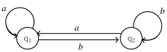
Fig. 3: Finite, non-blocking alternating transition system

Example 4.2.

Consider a finite, non-blocking alternating transition system

$T=(\{q_{1},q_{2}\},\{a,b\},\{1\},\longrightarrow,\{q_{1},q_{2}\},1_{\{q_{1},q_{2}\}})$,

where $\longrightarrow$ is described by Fig 3. Since there only exists one disturbance label, we do not indicate it in this figure. A control strategy $f:\{q_{1},q_{2}\}^{+}\rightarrow\{a,b\}$ is defined as for any $s\in\{q_{1},q_{2}\}^{+}$,

$$f(s)=\left\{\begin{aligned} &b&\textrm{ if $|s|=n(n+3)/2-1$ for some $n\in\mathbb{N}$}\\ &a&\textrm{otherwise}\end{aligned}\right.$$

Define a family of finite sequences $s_{k}$ ($k\in\mathbb{N}$) as: $s_{1}=q_{1}q_{2}$ and for any $k>1$, $s_{k}=q_{1}s_{k-1}$. Let $\sigma=s_{1}s_{2}s_{3}\cdots$. Thus $\sigma\neq\sigma[1,n](\sigma[n+1,m])^{\omega}$ for any $n,m\in\mathbb{N}$ with $n<m$. It is easy to check that $Out(q_{1},f)=\{\sigma\}$.

Now we show that there does not exist a reactive plan such that $\sigma$ is a trajectory generated by this plan. Suppose that $\sigma$ is generated by the reactive plan $RP=\{(1,q_{1},a_{1},N_{1}),(2,q_{2},a_{2},N_{2}),\cdots,(k,q_{k},a_{k},N_{k})\}$. Then there exists a sequence $\sigma_{N}=i_{1}i_{2}\cdots$ over $\{1,2,\cdots,k\}$ such that $i_{1}=1$ and for all $j\in\mathbb{N}$, $q_{i_{j}}=\sigma[j]$ and $i_{j+1}\in N_{i_{j}}$. Since $\{1,2,\cdots,k\}$ is a finite set, we have $i_{l}=i_{m}$ for some $l<m$. On the other hand, since $T$ is determined, we get $N_{i_{j}}=\{i_{j+1}\}$ for all $j\in\mathbb{N}$. Further, it follows from $i_{l}=i_{m}$ that $i_{l+1}=i_{m+1}$. Similarly, we have $i_{l+j}=i_{m+j}$ for all $j\in\mathbb{N}$. Thus $\sigma_{N}=i_{1}i_{2}\cdots i_{l}\circ(i_{l+1}\cdots i_{m})^{\omega}$ and then $\sigma=q_{i_{1}}q_{i_{2}}\cdots q_{i_{l}}\circ(q_{i_{l+1}}\cdots q_{i_{m}})^{\omega}$. This contradicts that for any $n,m\in\mathbb{N}$ with $n<m$, $\sigma\neq\sigma[1,n]\sigma[n+1,m]^{\omega}$.

5 Correctness and completeness of control strategy algorithm

The previous section presents a control strategy algorithm to solve Problem 1. This section will deal with its correctness and completeness. The former is ensured by the result below.

Theorem 21.

Given a finite, non-blocking alternating transition system $T=(Q,A,B,\longrightarrow,O,H)$, an LTL${}_{-X}(\mathbb{P})$ formula $\phi$ and a valuation function $\prod:Q\rightarrow 2^{\mathbb{P}}$, if control strategy algorithm returns a state $q_{0}$ and a control strategy $f_{RP}$, then $\sigma\models\phi$ for any $\sigma\in Out(q_{0},f_{RP})$.

Proof.

Suppose that control strategy algorithm returns a state $q_{0}$ and a control strategy $f_{RP}$. Then by Algorithm 1, a reactive plan $RP$ satisfying $\phi$ is found. Thus by Theorem 16 and 19, we have $\sigma\models\phi$ for any $\sigma\in Out(q_{0},f_{RP})$. ∎

The rest of this section concerns itself with the completeness of control strategy algorithm. That is, we consider the following question: given a finite, non-blocking alternating transition system $T$ and an LTL${}_{-X}(\mathbb{P})$ formula $\phi$, whether this algorithm must can find an initial state and a control strategy for $T$ enforcing $\phi$ if such state and control strategy exist? We will provide a partial answer for this question. Before dealing with this issue, some related notions and results are recalled.

Definition 22.

A B$\ddot{u}$chi automaton is a tuple $\mathcal{A}=(S,S_{0},L,\rightarrow_{\mathcal{A}},F)$, where

$\bullet$ $S$ is a finite set of states;

$\bullet$ $S_{0}\subseteq S$ is a set of initial states;

$\bullet$ $L$ is an input alphabet;

$\bullet$ $\rightarrow_{\mathcal{A}}\subseteq S\times L\times S$ is a transition relation;

$\bullet$ $F\subseteq S$ is a set of accepting states.

An infinite sequence $\sigma\in S^{\omega}$ is said to be a run accepted by $\mathcal{A}$ if and only if $\sigma[1]\in S_{0}$, $\sigma[i]\xrightarrow{a_{i}}_{\mathcal{A}}\sigma[i+1]$ for all $i\in\mathbb{N}$ and there exists $x\in F$ such that $x$ appears infinitely often in $\sigma$.

The B$\ddot{u}$chi automaton $\mathcal{A}$ is said to be total if both $S_{0}$ and $\{x^{\prime}:x\xrightarrow{l}x^{\prime}\}$ are singleton sets for any $x\in S$ and $l\in L$.

Definition 23.

Let $\mathcal{A}=(S,S_{0},L,\rightarrow_{\mathcal{A}},F)$ be a B$\ddot{u}$chi automaton. An infinite sequence $\sigma_{L}\in L^{\omega}$ is accepted by the B$\ddot{u}$chi automaton $\mathcal{A}$ if and only if there exists a run $\sigma$ accepted by $\mathcal{A}$ such that $\sigma[i]\xrightarrow{\sigma_{L}[i]}_{\mathcal{A}}\sigma[i+1]$ for all $i\in\mathbb{N}$.

In [31], it was proven that for any LTL${}_{-X}(\mathbb{P}$) formula $\phi$, there exists a B$\ddot{u}$chi automaton $\mathcal{A}_{\phi}$ with input alphabet $2^{\mathbb{P}}$ which accepts exactly the sequences $\sigma\in(2^{\mathbb{P}})^{\omega}$ satisfying formula $\phi$. The interested reader is referred to [10, 11, 26, 31, 32] for this topic.

Definition 24.

Let $\mathbb{P}$ be a set of atomic propositions. An LTL${}_{-X}(\mathbb{P})$ formula $\phi$ is said to be total if there exists a total B$\ddot{u}$chi automaton $\mathcal{A}_{\phi}$ with input alphabet $2^{\mathbb{P}}$ such that $\mathcal{A}_{\phi}$ accepts exactly the sequences $\sigma\in(2^{\mathbb{P}})^{\omega}$ satisfying $\phi$.

Adopting the tool LTL2BA provided by Oddoux and Gastin [22], we may check that the following formulae are total: $p_{1}\mathbf{U}p_{2}$, $\Box(p_{1}\mathbf{U}p_{2})$, $\diamond(p_{1}\mathbf{U}p_{2})$, $\Box(p_{1}\rightarrow p_{2})$, $\Box\diamond(p_{1}\rightarrow p_{2})$, $\Box(p_{1}\rightarrow\diamond p_{2})$, $\diamond p\wedge\diamond q\wedge\diamond t\wedge\diamond r$, and so on . Some of these formula are considered as control specifications in [9].

Convention. For convenience, for any total LTL${}_{-X}(\mathbb{P})$ formula $\phi$, $\mathcal{A}_{\phi}$ denotes a total B$\ddot{u}$chi automaton with input alphabet $2^{\mathbb{P}}$ which accepts exactly the sequences $\sigma\in(2^{\mathbb{P}})^{\omega}$ satisfying $\phi$.

In the remainder of this section, we will prove that the control strategy algorithm in Algorithm 1 is complete w.r.t. total LTL${}_{-X}(\mathbb{P})$ formulae. Formally, we want to demonstrate that, given a finite, non-blocking alternating transition system $T$, an LTL${}_{-X}(\mathbb{P})$ formula $\phi$ and a valuation function $\prod$, if $\phi$ is total and there exists a state $q_{0}$ and a control strategy $f_{0}$ so that $\sigma\models\phi\textrm{ for all }\sigma\in Out(q_{0},f_{0})$, then the control strategy algorithm can find an initial state $q$ and a control strategy $f$ of $T$ enforcing $\phi$. According to Corollary 20, it is enough to prove that there exists a reactive plan of $T$ satisfying $\phi$. So in the rest of this section, we will construct such reactive plan. The desired reactive plan will be obtained from the production automaton of $T$ and $\mathcal{A}_{\phi}$ defined below. Similar constructions have appeared in [9, 17, 27].

Definition 25.

Let $T=(Q,A,B,{\longrightarrow,}O,H)$ be a finite, non-blocking alternating transition system, $q_{0}\in Q$, $\phi$ a total LTL${}_{-X}(\mathbb{P})$ formula, ${\mathcal{A}_{\phi}=(S,\{x_{0}\},2^{\mathbb{P}},\rightarrow_{\mathcal{A}_{\phi}},F)}$ and let $\prod:Q\rightarrow 2^{\mathbb{P}}$ be a valuation function. The product automaton of the pair $(T,q_{0})$ and $\mathcal{A}_{\phi}$ is defined as $\mathcal{A}_{T,q_{0}}^{\phi}=(S_{T},S_{T}^{0},A,B,\rightarrow,F_{T})$, where

$\bullet$ $S_{T}=Q\times S$;

$\bullet$ $S_{T}^{0}=\{(q_{0},x_{0})\}$;

$\bullet$ $\rightarrow\subseteq S_{T}\times A\times B\times S_{T}$ is a transition relation defined as: $(q,x)\xrightarrow{a,b}(q^{\prime},x^{\prime})$ if and only if $q\xrightarrow{a,b}q^{\prime}$ and $x\xrightarrow{\prod(q)}_{\mathcal{A_{\phi}}}x^{\prime}$;

$\bullet$ $F_{T}=Q\times F$ is a set of accepting states of $\mathcal{A}_{T,q_{0}}^{\phi}$.

An infinite sequence $\sigma_{T}\in(S_{T})^{\omega}$ is said to be a run accepted by $\mathcal{A}_{T,q_{0}}^{\phi}$ if and only if the following hold:

(1) $\sigma_{T}[1]\in S_{T}^{0}$,

(2) for all $i\in\mathbb{N}$, $\sigma_{T}[i]\xrightarrow{a_{i},b_{i}}\sigma_{T}[i+1]$ for some $a_{i}\in A$ and $b_{i}\in B$, and

(3) there exists $(q,x)\in F_{T}$ such that $(q,x)$ appears infinitely often in $\sigma_{T}$.

It is clear that the sets $S_{T}$ and $F_{T}$ are finite. For any (finite or infinite) sequence $\alpha_{T}=(q_{1},x_{1})(q_{2},x_{2})\cdots$ over $S_{T}$, we define the projections $\Upsilon_{T}(\alpha_{T})=q_{1}q_{2}\cdots$ and $\Upsilon_{A}(\alpha_{T})=x_{1}x_{2}\cdots$.

Lemma 26.

[9, 17] The projection $\Upsilon_{T}(\sigma_{T})$ of any accepted run $\sigma_{T}$ of $\mathcal{A}_{T,q_{0}}^{\phi}$ is a trajectory of $T$ satisfying $\phi$.

Clearly, for any control strategy $f:Q^{+}\rightarrow A$ of $T$, the function $f_{T}:(S_{T})^{+}\rightarrow A$ defined as $f_{T}\triangleq f\circ\Upsilon_{T}$ is a control strategy of $\mathcal{A}_{T,q_{0}}^{\phi}$. The outcome $Out_{\mathcal{A}_{T,q_{0}}^{\phi}}((q_{0},x_{0}),f_{T})$ of $f_{T}$ from $(q_{0},x_{0})$ is defined as $Out_{\mathcal{A}_{T,q_{0}}^{\phi}}((q_{0},x_{0}),f_{T})\triangleq\{\sigma_{T}\in(S_{T})^{\omega}:\sigma_{T}[1]=(q_{0},x_{0})\ \mathrm{and}\ {\forall i\in\mathbb{N}{\exists b_{i}}\in B}(\sigma_{T}[i]\xrightarrow{f_{T}(\sigma_{T}[1,i]),b_{i}}\sigma_{T}[i+1])\}\}$. Similarly, we may define $Out_{\mathcal{A}_{T,q_{0}}^{\phi}}^{n}((q_{0},x_{0}),f_{T})$ ($n\in\mathbb{N}$), $Out_{\mathcal{A}_{T,q_{0}}^{\phi}}^{+}((q_{0},x_{0}),f_{T})$ and $Out_{\mathcal{A}_{T,q_{0}}^{\phi}}^{\infty}((q_{0},x_{0}),f_{T})$. For simplicity, we often omit the subscripts in them.

Lemma 27.

Let $T=(Q,A,B,{\longrightarrow,}O,H)$ be a finite, non-blocking alternating transition system, $q_{0}\in Q$, $\phi$ a total LTL${}_{-X}(\mathbb{P})$ formula and let $\prod$ be a valuation function. Suppose that $\mathcal{A}_{T,q_{0}}^{\phi}=(S_{T},S_{T}^{0},A,B,\rightarrow,F_{T})$ is the product automaton of the pair $(T,q_{0})$ and $\mathcal{A}_{\phi}$ and $f_{0}$ is a control strategy of $T$ so that $\sigma\models\phi$ for all $\sigma\in Out(q_{0},f_{0})$. Then, for control strategy $f_{T}:(S_{T})^{+}\rightarrow A$ with $f_{T}\triangleq f_{0}\circ\Upsilon_{T}$, we have

(1) $\alpha_{T}\in Out^{\infty}((q_{0},x_{0}),f_{T})$ implies $\Upsilon_{T}(\alpha_{T})\in Out^{\infty}(q_{0},f_{0})$,

(2) for any $\sigma_{T}\in Out((q_{0},x_{0}),f_{T})$, $\sigma_{T}$ is accepted by $\mathcal{A}_{T,q_{0}}^{\phi}$.

Proof.

Let $f_{T}=f_{0}\circ\Upsilon_{T}$. Then (1) follows from $f_{T}=f_{0}\circ\Upsilon_{T}$, Definition 25 and the definition of outcomes. Next, we prove (2). Let $\sigma_{T}\in Out((q_{0},x_{0}),f_{T})$. Then by Definition 25 and the definition of $Out((q_{0},x_{0}),f_{T})$, it is enough to show that there exists $(q,x)\in F_{T}$ such that $(q,x)$ appears infinitely often in $\sigma_{T}$. By (1) and $\sigma_{T}\in Out((q_{0},x_{0}),f_{T})$, we obtain $\Upsilon_{T}(\sigma_{T})\in Out(q_{0},f_{0})$. Then since $\sigma\models\phi\textrm{ for all }\sigma\in Out(q_{0},f_{0})$, $\prod(\Upsilon_{T}(\sigma_{T}))$ is accepted by $\mathcal{A}_{\phi}$. Moreover, it follows from Definition 25 that

$$\Upsilon_{A}(\sigma_{T})[i]\xrightarrow{\prod(\Upsilon_{T}(\sigma_{T}))[i]}_{\mathcal{A}_{\phi}}\Upsilon_{A}(\sigma_{T})[i+1]\textrm{ for all }i\in\mathbb{N}.$$ (1)

Further, since $\mathcal{A}_{\phi}$ is total, $\Upsilon_{A}(\sigma_{T})$ is a unique sequence satisfying (1). Then, since $\prod(\Upsilon_{T}(\sigma_{T}))$ is accepted by $\mathcal{A}_{\phi}$, $\Upsilon_{A}(\sigma_{T})$ is accepted by $\mathcal{A}_{\phi}$. Thus it follows that there exists $x\in F$ such that $x$ appears infinitely often in $\Upsilon_{A}(\sigma_{T})$. So, since $T$ is finite, there exists a state $q$ of $T$ such that $(q,x)$ appears infinitely often in $\sigma_{T}$.   ∎

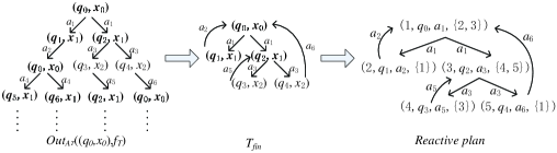
Fig. 4: Construction of reactive plan

In the following, we take two steps to construct the desired reactive plan. In the first step, we will construct a finite transition transition $T\!_{f\!i\!n}$ based on $Out^{\infty}((q_{0},x_{0}),f_{T})$ such that all trajectories of $T\!_{f\!i\!n}$ are runs accepted by $\mathcal{A}_{T,q_{0}}^{\phi}$. In the second step, we may easily obtain a reactive plan from $T\!_{f\!i\!n}$ so that the trajectories generated by this reactive plan are exactly the $\Upsilon_{T}-$projections of trajectories of $T_{f\!i\!n}$. Then by Lemma 26, this reactive plan satisfies $\phi$. Fig 4 illustrates these two steps. To construct the finite transition transition $T_{f\!i\!n}$, we introduce the following function.

Definition 28.

Let $T=(Q,A,B,{\longrightarrow,}O,H)$ be a finite, non-blocking alternating transition system, $q_{0}\in Q$, $\phi$ a total LTL${}_{-X}(\mathbb{P})$ formula and let $\prod$ be a valuation function. Suppose that $\mathcal{A}_{T,q_{0}}^{\phi}=(S_{T},S_{T}^{0},A,B,\rightarrow,F_{T})$ is the product automaton of the pair $(T,q_{0})$ and $\mathcal{A}_{\phi}$, $f_{0}$ is a control strategy of $T$ and $f_{T}=f_{0}\circ\Upsilon_{T}$. The function $ReN:Out^{\infty}((q_{0},x_{0}),f_{T})\rightarrow\mathbb{N}\cup\{\infty\}$ is defined as for any $\alpha_{T}\in Out^{\infty}((q_{0},x_{0}),f_{T})$,

$$ReN(\alpha_{T})=\inf\{n:\textrm{there exist }i<n\textrm{ such that }\alpha_{T}[i]=\alpha_{T}[n]\in F_{T}\}.$$

Here, inf$\emptyset=\infty$. Intuitively, $ReN(\alpha_{T})<\infty$ means that there exists an accepting state in $F_{T}$ occurring in $\alpha_{T}$ at least two times. Given a run $\sigma_{T}$ accepted by $\mathcal{A}_{T,q_{0}}^{\phi}$, by Definition 25 and 28, we have $\sigma_{T}[j]=\sigma_{T}[n]\in F_{T}$ for some $j<n$ and then $ReN(\sigma_{T})=n<\infty$. It is easy to check that $\sigma_{T}[1,j]\circ(\sigma_{T}[j+1,n])^{\omega}$ is also a run accepted by $\mathcal{A}_{T,q_{0}}^{\phi}$, where $(\sigma_{T}[j+1,n])^{\omega}\triangleq\sigma_{T}[j+1,n]\circ\sigma_{T}[j+1,n]\circ\cdots$. Inspired by this fact, we will construct a finite transition transition $T_{f\!i\!n}$ based on $Out^{\infty}((q_{0},x_{0}),f_{T})$ such that the trajectories of $T_{f\!i\!n}$ are runs accepted by $\mathcal{A}_{T,q_{0}}^{\phi}$.

Definition 29.

Let $T=(Q,A,B,{\longrightarrow,}O,H)$ be a finite, non-blocking alternating transition system, $q_{0}\in Q$, $\phi$ a total LTL${}_{-X}(\mathbb{P})$ formula and let $\prod$ be a valuation function. Suppose that $\mathcal{A}_{T,q_{0}}^{\phi}=(S_{T},S_{T}^{0},A,B,\rightarrow,F_{T})$ is the product automaton of the pair $(T,q_{0})$ and $\mathcal{A}_{\phi}$, $f_{0}$ is a control strategy of $T$ and $f_{T}=f_{0}\circ\Upsilon_{T}$. The accepting transition system w.r.t. $\mathcal{A}_{T,q_{0}}^{\phi}$ and $f_{T}$ is defined as

$T_{fin}(\mathcal{A}_{T,q_{0}}^{\phi},f_{T})=<S_{f},A,\rightarrow_{f},lab>$,

where

$\bullet$ $S_{f}=\{s_{T}\in Out^{+}((q_{0},x_{0}),f_{T}):ReN(s_{T})=\infty\}$. That is, the set $S_{f}$ contains all $s_{T}\in Out^{+}((q_{0},x_{0}),f_{T})$ in which each accepting state occurs at most one time;

$\bullet$ $\rightarrow_{f}\subseteq S_{f}\times A\times S_{f}$ is a transition relation defined as: $s_{T}\xrightarrow{a}_{f}s_{T}^{\prime}$ if and only if $a=f_{T}(s_{T})$ and for some $(q,x)\in S_{T}$ and $b\in B$, $s_{T}[end]\xrightarrow{a,b}(q,x)$ and one of the following holds:

(1) $s_{T}\circ(q,x)=s_{T}^{\prime}$, or

(2) $ReN(s_{T}\circ(q,x))<\infty$, $s_{T}^{\prime}\prec s_{T}\circ(q,x)$ and $s_{T}^{\prime}[end]=(q,x)$ ;

$\bullet$ $lab:S_{f}\rightarrow S_{T}$ is a label function defined as: for any $s_{T}\in S_{f}$, $lab(s_{T})=s_{T}[end]$.

An infinite sequence $\sigma_{T}\in(S_{T})^{\omega}$ is said to be a trajectory of $T_{f\!i\!n}(\mathcal{A}_{T,q_{0}}^{\phi},f_{T})$ if and only if there exists an infinite sequence $s_{T}^{1}s_{T}^{2}\cdots$ over $S_{f}$ such that $s_{T}^{1}=(q_{0},x_{0})$ and for any $i\in\mathbb{N}$, $lab(s_{T}^{i})=\sigma_{T}[i]$ and $s_{T}^{i}\xrightarrow{a_{i}}_{f}s_{T}^{i+1}$.

The left and middle figures in Fig 4 illustrate the above construction. In this figure, the nodes labeled by accepting states of $\mathcal{A}_{T,q_{0}}^{\phi}$ are identified in boldface type. In the left figure in Fig 4, consider the trajectory $\sigma_{T}=(q_{0},x_{0})(q_{1},x_{1})(q_{0},x_{0})(q_{5},x_{1})\cdots$. Clearly, none of accepting states occurs in $\sigma_{T}[1]$ or $\sigma_{T}[1,2]$ two times, while the accepting state $(q_{0},x_{0})$ occurs in $\sigma_{T}[1,3]$ two times. Thus by Definition 28 and 29, we have $\sigma_{T}[1],\sigma_{T}[1,2]\in S_{f}$ and $\sigma_{T}[1,3]\not\in S_{f}$. Then $\sigma_{T}[1]$ and $\sigma_{T}[1,2]$ are labeled by $(q_{0},x_{0})$ and $(q_{1},x_{1})$, respectively. Furthermore, by the definition of $\rightarrow_{f}$, one may check that $\sigma_{T}[1]\xrightarrow{a_{1}}_{f}\sigma_{T}[1,2]$ and $\sigma_{T}[1,2]\xrightarrow{a_{2}}_{f}\sigma_{T}[1]$.

The following result reveals that the state set of $T_{fin}(\mathcal{A}_{T,q_{0}}^{\phi},f_{T})$ is finite and its trajectories are runs accepted by $\mathcal{A}_{T,q_{0}}^{\phi}$.

Lemma 30.

Let $T=(Q,A,B,{\longrightarrow,}O,H)$ be a finite, non-blocking alternating transition system, $q_{0}\in Q$, $\phi$ a total LTL${}_{-X}(\mathbb{P})$ formula and let $\prod$ be a valuation function. Suppose that $\mathcal{A}_{T,q_{0}}^{\phi}$ is the product automaton of the pair $(T,q_{0})$ and $\mathcal{A}_{\phi}$ and $f_{0}$ is a control strategy of $T$ so that $\sigma\models\phi$ for all $\sigma\in Out(q_{0},f_{0})$. Let $f_{T}=f_{0}\circ\Upsilon_{T}$ and let $T_{fin}(\mathcal{A}_{T,q_{0}}^{\phi},f_{T})=<S_{f},A,\rightarrow_{f},lab>$ be the accepting transition system w.r.t. $\mathcal{A}_{T,q_{0}}^{\phi}$ and $f_{T}$. Then the following conclusions hold:

(1) The set $S_{f}$ is finite and non-empty.

(2) The trajectory $\sigma_{T}$ of $T_{f\!i\!n}(\mathcal{A}_{T,q_{0}}^{\phi},f_{T})$ is a run accepted by $\mathcal{A}_{T,q_{0}}^{\phi}$.

(3) For any $s_{T}\in S_{f}$ and for any state $q$ of $T$, if $\Upsilon_{T}(s_{T}[end])\xrightarrow{f_{T}(s_{T}),b}q$ for some $b\in B$, then there exists $s_{T}^{\prime}\in S_{f}$ such that $s_{T}\xrightarrow{f_{T}(s_{T})}_{f}s_{T}^{\prime}$ and ${\Upsilon_{T}(s_{T}^{\prime})[end]=q}$.

Proof.

See Appendix A.   ∎

Now we may generate the desired reactive plan from $T_{f\!i\!n}(\mathcal{A}_{T,q_{0}}^{\phi},f_{T})$.

Definition 31.

Let $T$ be a finite, non-blocking alternating transition system, $q_{0}$ a state $T$, $\phi$ a total LTL${}_{-X}(\mathbb{P})$ formula and let $\prod$ be a valuation function. Suppose that $\mathcal{A}_{T,q_{0}}^{\phi}$ is the product automaton of the pair $(T,q_{0})$ and $\mathcal{A}_{\phi}$ and $f_{0}$ is a control strategy of $T$ so that $\sigma\models\phi$ for all $\sigma\in Out(q_{0},f_{0})$. Let $f_{T}=f_{0}\circ\Upsilon_{T}$ and let $T_{fin}(\mathcal{A}_{T,q_{0}}^{\phi},f_{T})=<S_{f},A,\rightarrow_{f},lab>$ be the accepting transition system w.r.t. $\mathcal{A}_{T,q_{0}}^{\phi}$ and $f_{T}$ with $S_{f}=\{s^{1}_{T},s^{2}_{T},\cdots,s^{m}_{T}\}$ and $s^{1}_{T}=(q_{0},x_{0})$. Then the set $RP(T_{fin})$ consists of all SCRs $(i,\Upsilon_{T}(s^{i}_{T}[end]),a_{i},N_{i})$ such that

(1) $1\leq i\leq m$,

(2) $a_{i}=f_{T}(s^{i}_{T})$, and

(3) $N_{i}=\{j\in\mathbb{N}:s^{i}_{T}\xrightarrow{a_{i}}_{f}s^{j}_{T}\}$.

The right in Fig 4 illustrates the above construction w.r.t. $T_{f\!i\!n}$ (i.e., the middle one in Fig 4). In this figure, each plan state corresponds to a unique state of $T_{f\!i\!n}$ and the action to be executed in each plan state is set to be the one in the corresponding state of $T_{f\!i\!n}$. According to (3) in Lemma 30 and Definition 5, $RP(T_{fin})$ defined above is a reactive plan. In the following, we demonstrate that this reactive plan satisfies $\phi$.

Theorem 32.

Let $T=(Q,A,B,{\longrightarrow,}O,H)$ be a finite, non-blocking alternating transition system, $q_{0}\in Q$, $\phi$ a total LTL${}_{-X}(\mathbb{P})$ formula and let $\prod:Q\rightarrow 2^{\mathbb{P}}$ be a valuation function. Suppose that $\mathcal{A}_{T,q_{0}}^{\phi}$ is the product automaton of the pair $(T,q_{0})$ and $\mathcal{A}_{\phi}$ and $f_{0}$ is a control strategy of $T$ so that $\sigma\models\phi$ for all $\sigma\in Out(q_{0},f_{0})$. Let $f_{T}=f_{0}\circ\Upsilon_{T}$, $T_{fin}(\mathcal{A}_{T,q_{0}}^{\phi},f_{T})$ the accepting transition system w.r.t. $\mathcal{A}_{T,q_{0}}^{\phi}$ and $f_{T}$ and let $RP(T_{fin})=\{(i,\Upsilon_{T}(s^{i}_{T}[end]),a_{i},N_{i}):1\leq i\leq m\}$ be the reactive plan defined by Definition 31. Then for any trajectory $\sigma$ generated by the reactive plan $RP(T_{fin})$, we have $\sigma\models\phi$.

Proof.

Let $\sigma$ be a trajectory generated by the reactive plan $RP(T_{fin})$. So by Definition 6, there exists an infinite sequence $i_{1}i_{2}\cdots$ of plan states in $RP(T_{fin})$ such that

$$i_{1}=1,\sigma[j]=\Upsilon_{T}(s^{i_{j}}_{T}[end])\textrm{ and }i_{j+1}\in N_{i_{j}}\textrm{ for all }j\in\mathbb{N}.$$ (2)

We set $\sigma_{T}=s^{i_{1}}_{T}[end]s^{i_{2}}_{T}[end]\cdots$. Clearly, $\Upsilon_{T}(\sigma_{T})=\sigma$. Therefore, by Lemma 26 and 30, in order to prove $\sigma\models\phi$, it suffices to show that $\sigma_{T}$ is a trajectory of $T_{fin}(\mathcal{A}_{T,q_{0}}^{\phi},f_{T})$.

It follows from $i_{1}=1$ and Definition 31 that $s^{i_{1}}_{T}=(q_{0},x_{0})$. Let $j\in\mathbb{N}$. By (2), we have $i_{j+1}\in N_{i_{j}}$. Further, it follows from Definition 29 and 31 that $s^{i_{j}}_{T}\xrightarrow{a_{i_{j}}}_{f}s^{i_{j+1}}_{T}$. Thus by Definition 29, $\sigma_{T}$ is a trajectory of $T_{fin}(\mathcal{A}_{T,q_{0}}^{\phi},f_{T})$, as desired.   ∎

Now we arrive at the main result of this section.

Theorem 33.

For any finite, non-blocking alternating transition system $T=(Q,A,B,{\longrightarrow,}O,H)$, LTL${}_{-X}(\mathbb{P})$ formula $\phi$ and valuation function $\prod$, if $\phi$ is total and there exists a state $q$ of $T$ and a control strategy $f:Q^{+}\rightarrow A$ such that $\sigma\models\phi$ for all $\sigma\in Out(q,f)$, then the control strategy algorithm can find an initial state $q^{\prime}$ and a control strategy $f^{\prime}:Q^{+}\rightarrow A$ so that $\sigma\models\phi$ for all $\sigma\in Out(q^{\prime},f^{\prime})$.

Proof.

Let $T=(Q,A,B,\rightarrow,O,H)$ be a finite, non-blocking alternating transition system, $\phi$ an LTL${}_{-X}(\mathbb{P})$ formula and $\prod:Q\rightarrow 2^{\mathbb{P}}$ a valuation function. Suppose that $\phi$ is total and there exists a state $q$ of $T$ and a control strategy $f:Q^{+}\rightarrow A$ such that $\sigma\models\phi$ for all $\sigma\in Out(q,f)$. Then, by Theorem 32 and Definition 29 and 31, there exists a reactive plan $RP(T_{fin})$ of $T$ such that all trajectories generated by this reactive plan satisfy $\phi$. Therefore, by Corollary 20, the control strategy algorithm can find an initial state $q^{\prime}$ and a control strategy $f_{RP}:Q^{+}\rightarrow A$ so that $\sigma\models\phi$ for all $\sigma\in Out(q^{\prime},f_{RP})$.   ∎

6 Conclusion and future work

Pola and Tabuada have introduced finite abstractions for control systems $\Sigma$ with disturbance inputs [23, 24]. However, since these finite abstractions are modeled by finite, non-blocking alternating transition systems rather than usual transition systems, the approaches provided in [9][27][29] are not suitable for finding control strategies for Pola and Tabuada’s abstractions. To overcome this defect, this paper presents a control strategy algorithm based on Kabanza et al.’s planning algorithm (see Algorithm 1). This control strategy algorithm can be used to find an initial state and a control strategy of finite, non-blocking alternating transition system enforcing an given LTL_-X formula. The correctness and completeness of this algorithm are explored. We demonstrate that this algorithm is correct (see Theorem 21) and is complete w.r.t total LTL_-X formulas (see Theorem 33). But it is still an open problem: whether Theorem 33 holds for all LTL_-X formulas. We will explore this problem in further work.

Now, we may adopt the control strategy algorithm to find an initial state and a control strategy of Pola and Tabuada’s finite abstraction enforcing an LTL_-X formula $\phi$. However, the control problem in the design of control system is:

Problem 2.

Given a control system $\Sigma$ with disturbance inputs and an LTL_-X formula $\varphi$ as specification, how to construct a feedback controller such that all trajectories of $\Sigma$ with this controller satisfy $\varphi$ even in the presence of disturbance inputs?

Thus a natural question arises at this point: if an initial state and a control strategy of finite abstraction enforcing an LTL_-X formula $\varphi$ have been found, whether the controller for finite abstraction can be applied to the original systems to meet $\varphi$? We have dealt with this problem in [33].

Appendix A

In this appendix, we fix a finite, non-blocking alternating transition system $T=(Q,A,B,{\longrightarrow,}O,H)$, an initial state $q_{0}\in Q$, a total LTL${}_{-X}(\mathbb{P})$ formula $\phi$, $\mathcal{A}_{\phi}=(S,\{x_{0}\},2^{\mathbb{P}},\rightarrow_{\mathcal{A}_{\phi}},F)$, a valuation function $\prod:Q\rightarrow 2^{\mathbb{P}}$, a control strategy $f_{0}:Q^{+}\rightarrow A$ such that $\sigma\models\phi$ for all $\sigma\in Out(q_{0},f_{0})$. Suppose that ${\mathcal{A}_{T,q_{0}}^{\phi}=(S_{T},S_{T}^{0},A,B,\rightarrow,F_{T})}$ is the product automaton of the pair $(T,q_{0})$ and $\mathcal{A}_{\phi}$ (see Definition 25), and the control strategy $f_{T}:(S_{T})^{+}\rightarrow A$ is defined as $f_{T}\triangleq f_{0}\circ\Upsilon_{T}$. Before proving Lemma 30, we provide two auxiliary results.

Lemma A.1.

(1) For any $\sigma\in Out(q_{0},f_{0})$, there exists a unique $\sigma_{T}\in Out((q_{0},x_{0}),f_{T})$ such that $\Upsilon_{T}(\sigma_{T})=\sigma$.

(2) For any $s\in Out^{+}(q_{0},f_{0})$, there exists a unique $s_{T}\in Out^{+}((q_{0},x_{0}),f_{T})$ such that $\Upsilon_{T}(s_{T})=s$.

(3) For any $\alpha_{T}\in Out^{\infty}((q_{0},x_{0}),f_{T})$, if $ReN(\alpha_{T})=n$ then for any $k<n$, $ReN(\alpha_{T}[1,k])=\infty$.

Proof.

(1) Let $\sigma\in Out(q_{0},f_{0})$. Then $\sigma\models\phi$. It follows from Definition 4 that $\prod(\sigma)\models\phi$. Then $\prod(\sigma)$ is accepted by $\mathcal{A}_{\phi}$. Thus by Definition 22 and 23, there exists a run $x_{1}x_{2}\cdots\in S^{\omega}$ accepted by $\mathcal{A}_{\phi}$ such that

$$x_{1}=x_{0}\textrm{ and }x_{i}\xrightarrow{\prod(\sigma[i])}_{\mathcal{A}_{\phi}}x_{i+1}\ \textrm{for all }i\in\mathbb{N}.$$ (.3)

Moreover, it follows from $\sigma\in Out_{T}(q_{0},f_{0})$ that for any $i\in\mathbb{N}$, there exists $b_{i}\in B$ such that $\sigma[i]\xrightarrow{f_{0}(\sigma[1,i]),b_{i}}\sigma[i+1]$. This together with (.3) and Definition 25 implies that for any $i\in\mathbb{N}$,

$$(\sigma[i],x_{i})\xrightarrow{f_{0}(\sigma[1,i]),b_{i}}(\sigma[i+1],x_{i+1}).$$ (.4)

We set $\sigma_{T}=(\sigma[1],x_{1})(\sigma[2],x_{2})\cdots$. Clearly, $\Upsilon_{T}(\sigma_{T})=\sigma$ and $\sigma_{T}[1]=(q_{0},x_{0})$. Furthermore, since $f_{T}=f_{0}\circ\Upsilon_{T}$, we get $f_{T}(\sigma_{T}[1,i])=f_{0}(\sigma[1,i])$ for all $i\in\mathbb{N}$. Thus it follows from (.4) that for any $i\in\mathbb{N}$, $(\sigma[i],x_{i})\xrightarrow{f_{T}(\sigma_{T}[1,i]),b_{i}}(\sigma[i+1],x_{i+1})$. Therefore, we obtain $\sigma_{T}\in Out((q_{0},x_{0}),f_{T})$.

To show the uniqueness of such $\sigma_{T}$, let $\sigma_{T}^{\prime}\in Out((q_{0},x_{0}),f_{T})$ and $\Upsilon_{T}(\sigma_{T}^{\prime})=\sigma$. Then since $\mathcal{A}_{\phi}$ is total, there exists a unique run $x_{1}x_{2}\cdots$ such that $x_{1}=x_{0}$ and $x_{i}\xrightarrow{\prod(\sigma[i])}_{\mathcal{A}_{\phi}}x_{i+1}$ for all $i\in\mathbb{N}$. So by Definition 25, it is easy to check that $\Upsilon_{A}(\sigma_{T}^{\prime})=\Upsilon_{A}(\sigma_{T})$. Then it follows from $\Upsilon_{T}(\sigma_{T}^{\prime})=\sigma=\Upsilon_{T}(\sigma_{T})$ that $\sigma_{T}^{\prime}=\sigma_{T}$.

(2) Let $s\in Out^{+}(q_{0},f_{0})$. Then by the definition of $Out^{+}(q_{0},f_{0})$ and $Out(q_{0},f_{0})$, $s$ is a prefix of $\sigma$ for some $\sigma\in Out(q_{0},f_{0})$. So by (1), there exists $\sigma_{T}\in Out((q_{0},x_{0}),f_{T})$ such that $\Upsilon_{T}(\sigma_{T})=\sigma$ and $\sigma_{T}$ is accepted by $\mathcal{A}_{T,q_{0}}^{\phi}$. Thus we have $\Upsilon_{T}(\sigma_{T}[1,|s|])=s$ and $\sigma_{T}[1,|s|]\in Out^{+}((q_{0},x_{0}),f_{T})$. Similar to (1), we may show that $\sigma_{T}[1,|s|]$ is a unique sequence satisfying the condition.

(3) Follows from Definition 28.   ∎

Lemma A.2.

There exists $n\in\mathbb{N}$ such that for all $\sigma_{T}\in Out((q_{0},x_{0}),f_{T})$, we have $ReN(\sigma_{T})\leq n$.

Proof.

Suppose that for any $n\in\mathbb{N}$, there exists $\sigma^{n}_{T}\in Out((q_{0},x_{0}),f_{T})$ such that $ReN(\sigma^{n}_{T})>n$. We will give a contradiction. To this end, the following claim is provided first.

Claim. We may construct an infinite sequence $\sigma_{T}\in(S_{T})^{\omega}$ satisfying that for any $k\in\mathbb{N}$, there exist $k_{i}\in\mathbb{N}(i\in\mathbb{N})$ with $k_{1}<k_{2}<k_{3}<\cdots$ such that $\sigma^{k_{i}}_{T}[1,k]=\sigma_{T}[1,k]$ for any $i\in\mathbb{N}$.

We construct such a sequence by induction on $k$. Let $k=1$. We set $\sigma_{T}[1]=(q_{0},x_{0})$ and $k_{i}=i$ for each $i\in\mathbb{N}$. Then for any $i\in\mathbb{N}$, $\sigma^{k_{i}}_{T}[1]=\sigma^{i}_{T}[1]=(q_{0},x_{0})=\sigma_{T}[1]$ follows from $\sigma^{i}_{T}\in Out((q_{0},x_{0}),f_{T})$.

Suppose that $k=m+1$ and we have found $\sigma_{T}[1,m]$ and $m_{i}\in\mathbb{N}(i\in\mathbb{N})$ with $m_{1}<m_{2}<m_{3}<\cdots$ such that $\sigma^{m_{i}}_{T}[1,m]=\sigma_{T}[1,m]$ for all $i\in\mathbb{N}$. Since $S_{T}$ is finite, the set $\{\sigma^{m_{i}}_{T}[m+1]:i\in\mathbb{N}\}$ is finite. So there exists $(q_{k},x_{k})\in\{\sigma^{m_{i}}_{T}[m+1]:i\in\mathbb{N}\}$ and $k_{i}\in\{m_{1},m_{2},\cdots\}(i\in\mathbb{N})$ with $k_{1}<k_{2}<k_{3}<\cdots$ such that $\sigma^{k_{i}}_{T}[m+1]=(q_{k},x_{k})$ for all $i\in\mathbb{N}$. We set $\sigma_{T}[k]=(q_{k},x_{k})$. Thus it follows that $\sigma^{k_{i}}_{T}[1,k]=\sigma_{T}[1,m]\circ(q_{k},x_{k})=\sigma_{T}[1,k]$ for all $i\in\mathbb{N}$.

Now, we return to the proof of this lemma. It is easy to check that $\sigma_{T}\in Out((q_{0},x_{0}),f_{T})$. Then by Lemma 27, $\sigma_{T}$ is accepted by $\mathcal{A}_{T,q_{0}}^{\phi}$. To obtain a contradiction, we will show that $\sigma_{T}$ is not accepted by $\mathcal{A}_{T,q_{0}}^{\phi}$ below.

Let $k\in\mathbb{N}$. Since $k_{1}<k_{2}<\cdots$, there exists $i_{k}\in\{k_{1},k_{2},\cdots\}$ such that $i_{k}>k$. So by the above claim and the supposition at the beginning of the proof, we obtain $\sigma^{i_{k}}_{T}[1,k]=\sigma_{T}[1,k]$ and $ReN(\sigma^{i_{k}}_{T})>i_{k}>k$. Further, by Definition 28, we have $ReN(\sigma_{T})>i_{k}>k$. Then, since $k$ is an arbitrary nature number, we get $ReN(\sigma_{T})=\infty$. Since the accepting state set $F_{T}$ is finite, it follows from Definition 28 and $ReN(\sigma_{T})=\infty$ that there does not exist $(q,x)\in F_{T}$ such that $(q,x)$ appears infinitely often in $\sigma_{T}$. So $\sigma_{T}$ is not accepted by $\mathcal{A}_{T,q_{0}}^{\phi}$.   ∎

Lemma 30. Let $T=(Q,A,B,{\longrightarrow,}O,H)$ be a finite, non-blocking alternating transition system, $q_{0}\in Q$, $\phi$ a total LTL${}_{-X}(\mathbb{P})$ formula, $\mathcal{A}_{\phi}=(S,\{x_{0}\},2^{\mathbb{P}},\rightarrow_{\mathcal{A}_{\phi}},F)$ and let $\prod:Q\rightarrow 2^{\mathbb{P}}$ be a valuation function. Suppose that ${\mathcal{A}_{T,q_{0}}^{\phi}=(S_{T},S_{T}^{0},A,B,\rightarrow,F_{T})}$ is the product automaton of the pair $(T,q_{0})$ and $\mathcal{A}_{\phi}$ and $f_{0}$ is a control strategy of $T$ so that $\sigma\models\phi$ for all $\sigma\in Out(q_{0},f_{0})$. Let $f_{T}=f_{0}\circ\Upsilon_{T}$ and let $T_{fin}(\mathcal{A}_{T,q_{0}}^{\phi},f_{T})=<S_{f},\\ A,\rightarrow_{f},lab>$ be the accepting transition system w.r.t. $\mathcal{A}_{T,q_{0}}^{\phi}$ and $f_{T}$. Then the following conclusions hold:

(1) The set $S_{f}$ is finite and non-empty.

(2) The trajectory $\sigma_{T}$ of $T_{fin}(\mathcal{A}_{T,q_{0}}^{\phi},f_{T})$ is a run accepted by $\mathcal{A}_{T,q_{0}}^{\phi}$.

(3) For any $s_{T}\in S_{f}$ and for any state $q\in Q$ of $T$, if $\Upsilon_{T}(s_{T}[end])\xrightarrow{f_{T}(s_{T}),b}q$ for some $b\in B$, then there exists $s_{T}^{\prime}\in S_{f}$ such that $s_{T}\xrightarrow{f_{T}(s_{T})}_{f}s_{T}^{\prime}$ and ${\Upsilon_{T}(s_{T}^{\prime})[end]=q}$.

Proof.

(1) Clearly, $(q_{0},x_{0})\in S_{f}$ and then $S_{f}$ is non-empty. Next, we show that $S_{f}$ is finite. By Lemma A.2, there exists $n\in\mathbb{N}$ such that $ReN(\sigma_{T})\leq n$ for any $\sigma_{T}\in Out((q_{0},x_{0}),f_{T})$. Since $S_{T}=Q\times S$ is finite, $Out^{i}((q_{0},x_{0}),f_{T})$ is finite for any $i\in\mathbb{N}$ and then $\bigcup_{i<n}Out^{i}((q_{0},x_{0}),f_{T})$ is finite. So to complete the proof, we just need to show that $S_{f}\subseteq\bigcup_{i<n}Out^{i}((q_{0},x_{0}),f_{T})$.

Let $s_{T}\in S_{f}$. Then by Definition 29, we have $ReN(s_{T})=\infty$. On the other side, by Lemma 27, we obtain $\Upsilon_{T}(s_{T})\in Out^{+}(q_{0},f_{0})$. Then, since $T$ is non-blocking, by Definition 10, there exists $\sigma\in Out(q_{0},f_{0})$ such that $\Upsilon_{T}(s_{T})$ is a prefix of $\sigma$. Thus by Lemma A.1, there exists $\sigma_{T}\in Out((q_{0},x_{0}),f_{T})$ such that $s_{T}$ is a prefix of $\sigma_{T}$. Further, since $ReN(\sigma_{T})\leq n$ and $ReN(s_{T})=\infty$, by Definition 28, we get $|s_{T}|<ReN(\sigma_{T})\leq n$.

(2) Let $\sigma_{T}$ be a trajectory of $T_{fin}(\mathcal{A}_{T,q_{0}}^{\phi},f_{T})$. Then by (2) in Lemma 27, it is enough to show that $\sigma_{T}\in Out((q_{0},x_{0}),f_{T})$. By Definition 29, there exists a sequence $s_{T}^{1}s_{T}^{2}\cdots$ over $S_{f}$ such that

$s_{T}^{1}=(q_{0},x_{0})$ and for any $i\in\mathbb{N}$, $s_{T}^{i}[end]=\sigma_{T}[i]$ and $s_{T}^{i}\xrightarrow{a_{i}}_{f}s_{T}^{i+1}$.

Thus it follows from Definition 29 that $\sigma_{T}[1]=(q_{0},x_{0})$ and for any $i\in\mathbb{N}$, there exists $(q,x)\in S_{T}$ and $b\in B$ such that $a_{i}=f_{T}(s_{T}^{i})$, $\sigma_{T}[i]\xrightarrow{a_{i},b}(q,x)$ and $s_{T}^{i+1}[end]=\sigma_{T}[i+1]=(q,x)$. Then it follows that $\sigma_{T}\in Out((q_{0},x_{0}),f_{T})$.

(3) Let $s_{T}\in S_{f}$, $q\in Q$, $ReN(s_{T})=\infty$ and $\Upsilon_{T}(s_{T}[end])\xrightarrow{f_{T}(s_{T}),b}q$ for some $b\in B$. For convenience, we put $s=\Upsilon_{T}(s_{T})$. By (1) in Lemma 27, we have $s\in Out^{+}(q_{0},f_{0})$. Then it follows from $s[end]\xrightarrow{f_{T}(s_{T}),b}q$ and $f_{T}(s_{T})=f_{0}(s)$ that $sq\in Out^{+}(q_{0},f_{0})$. So by (2) in Lemma A.1, there exists a unique $s_{T}^{\prime}\in Out^{+}((q_{0},x_{0}),f_{T})$ such that $\Upsilon_{T}(s_{T}^{\prime})=sq$. Similarly, $s_{T}$ is a unique sequence in $Out^{+}((q_{0},x_{0}),f_{T})$ such that $\Upsilon_{T}(s_{T})=s$. Thus $s_{T}\circ(q,x)=s_{T}^{\prime}$ for some state $x\in S$ of $\mathcal{A}_{\phi}$. If $ReN(s_{T}^{\prime})=\infty$ then by Definition 29, we obtain $s_{T}^{\prime}\in S_{f}$, $s_{T}\xrightarrow{f_{T}(s_{T})}_{f}s_{T}^{\prime}$ and $\Upsilon_{T}(s_{T}^{\prime}[end])=q$. Suppose that $ReN(s_{T}^{\prime})<\infty$. Then since $ReN(s_{T})=\infty$ and $s_{T}\circ(q,x)=s_{T}^{\prime}$, by Definition 28, there exists $s_{T}^{\prime\prime}\prec s_{T}^{\prime}$ such that $s_{T}^{\prime\prime}[end]=s_{T}^{\prime}[end]$ and $ReN(s_{T}^{\prime\prime})=\infty$. Further, by Definition 29, we have $s_{T}^{\prime\prime}\in S_{f}$, $s_{T}\xrightarrow{f_{T}(s_{T})}_{f}s_{T}^{\prime\prime}$ and $\Upsilon_{T}(s_{T}^{\prime\prime}[end])=q$. ∎

References

[1]
R. Alur and T. A. Henzinger, Discrete abstractions of hybrid systems, in Proceedings of The IEEE, 88(7), 2000, pp. 971-984.
[2]
R. Alur and D. L. Dill, A theory of timed automata, Theoretical Computer Science, 126 (1994), pp. 183-235.
[3]
R. Alur, C. Courcoubetis, N. Halbwachs, T. A. Henzinger, P.-H. Ho, X. Nicollin, A. Olivero, J. Sifakis, and S. Yovine, The algorithmic analysis of hybrid systems, Theoretical Computer Science, 138 (1995), pp. 3-34.
[4]
M. Antoniotti and B. Mishra, Discrete Event Models + Temporal Logic = Supervisory Controller: Automatic Synthesis of Locomotion Controllers, in Proceedings of IEEE International Conference on Robotics and Automation, Nagoya-shi, Japan, 1995, pp. 1441-1446.
[5]
T. H. Cormen, C. E. Leiserson, R. L. Rivest, and C. Stein, Introduction to Algorithms, 2nd ed, Cambrideg, MA and New York: MIT Press and McGraw-Hill Book Company, 2001.
[6]
E. W. Dijkstra, A note on two problems in connexion with graphs, Numerische Mathematik, 1 (1959), pp.269-271.
[7]
E. A. Emerson, Temporal and modal logic, in Handbook of theoretical computer science: formal models and semantics, vol.B, J. van Leeuwen, Ed. Amsterdam, The Netherlands: North Holland/MIT Press, 1990, pp.995-1072.
[8]
G. E. Fainekos, H. Kress-Gazit, and G. J. Pappas, Temporal logic motion planning for mobile robots, in Proceedings of the 2005 IEEE International Conference on Robotics and Automation (ICRA), Barcelona, Spain, 2005, pp. 2020-2025.
[9]
G. E. Fainekos, H. Kress-Gazit, and G. J. Pappas, Hybrid controllers for path planning: A temporal logic approach, in Proceedings of 44th IEEE Conference on Decision and Control and 8th European Control Conference (CDC-ECC’05), vol.5, Seville, Spain, 2005, pp. 4885-4890.
[10]
P. Gastin and D. Oddoux, Fast LTL to Bchi automata translation, in Proceedings of 13th Conference on Computation Aided Verification (CAV 01), LNCS 2102, Paris, France, 2001, Springer-Verlag, pp. 53-65.
[11]
R. Gerth, D. Peled, M. Vardi, and P. Wolper, Simple on-the-fly automatic verification of linear temporal logic, in Proceedings of 15th IFIP WG6.1 International Symposium on Protocol Specification, Testing and Verification XV, London, U.K., 1996, pp. 3-18.
[12]
L. Habets and J. H. van Schuppen, A control problem for affine dynamical systems on a full-dimensional polytope, Automatica, 40 (2004), pp. 21-35.
[13]
L. Habets and J. H. van Schuppen, Control of piecewise-linear hybrid systems on simplices and rectangles, in Proceedings of Hybrid systems: Computation and control, LNCS 2034, Rome, Italy, 2001, Springer-Verlag, pp. 261-274.
[14]
T. A. Henzinger, P. W. Kopke, A. Puri, and P. Varaiya, What’s Decidable about Hybrid Automata?, Journal of Computer and System Sciences, 57 (1998), 94-124.
[15]
T. A. Henzinger and R. Majumdar, Symbolic model checking for rectangular hybrid systems, in Proceedings of the Sixth International Workshop on Tools and Algorithms for the Construction and Analysis of Systems, LNCS 1785, Berlin, Germany, 2000, Springer-Verlag, pp. 142-156.
[16]
F. Kabanza, M. Barbeau, and R. St-Denis, Planning control rules for reactive agents,
Artificial Intelligence, 95 (1997), pp. 67-113.
[17]
M. Kloetzer and C. Belta, A Fully Automated Framework for Control of Linear Systems from LTL Specifications, IEEE transactions on automatic control, 53 (2008), pp. 287-297.
[18]
X. Koutsoukos, P. Antsaklis, J. Stiver, and M. Lemmon, Supervisory control of hybrid systems, in Proceedings of the IEEE, 88 (2002), pp. 1026-1049.
[19]
B C. Kuo, Automatic control systems, Prentice-Hall, New York, 1975.
[20]
B. Lacerda and P. U Lima, Linear-Time Temporal Logic Control of Discrete Event Models of Cooperative Robots, Journal of Physical Agents, 2 (2008), pp. 53-61.
[21]
G. Lafferriere, G. J. Pappas, and S. Sastry, O-minimal hybrid systems, Mathematics of Control, Signals, and Systems, 13 (2000), pp. 1-21.
[22]
D. Oddoux and Paul Gastin, LTL 2 BA: fast translation from LTL formulae to Bchi automata, available at http://www.lsv.ens-cachan.fr/ gastin/ltl2ba/.
[23]
G. Pola and P. Tabuada, Symbolic models for nonlinear control systems: Alternating approximate bisimulations,
SIAM Journal on Control and Optimization, 48 (2009), pp. 719-733.
[24]
G. Pola and P. Tabuada, Symbolic models for nonlinear control systems affected by disturbances, in Proceedings of 47th IEEE Conference on Decision and Control, Cancun, Mexico, 2008, pp. 251-256.
[25]
G. Pola, A. Girard, and P. Tabuada, Approximately bisimilar symbolic models for nonlinear control systems, Automatica, 44 (2008), pp. 2508-2516.
[26]
F. Somenzi and R. Bloem, Efficient bchi automata from LTL formulae, in Proceedings of the 12th International Conference on Computer Aided Verification, LNCS 1855, Chicago, USA, 2000, Springer-Verlag, pp. 248 - 263.
[27]
P. Tabuada and G. J. Pappas, Linear time logic control of discrete-time linear systems, IEEE Transactions on Automatic Control, 51(12), 2006, pp. 1862-1877.
[28]
P. Tabuada and G. J. Pappas, Finite bisimulations of controllable linear systems, in Proceedings of the 42nd IEEE Conference on Decision and Control, Hawaii, USA, 2003, pp. 634-639.
[29]
P. Tabuada and G. J. Pappas, From discrete specifications to hybrid control, in Proceedings of the 42nd IEEE Conference on Decision and Control, Hawaii, USA, 2003, pp. 3366-3371.
[30]
P. Tabuada, Symbolic models for control systems, Acta Informatica, 43 (2007), pp. 477-500.
[31]
P. Wolper, M. Vardi, and A. Sistla, Reasoning about infinite computation paths, in Proceedings of 24th IEEE Annual Symposium on Foundations of Computer Science, Tucson, USA, 1983, pp. 185-194.
[32]
P. Wolper, Constructing automata from temporal logic formulas: A tutorial, in Proceedings of Lectures Formal Methods Performance Analysis: First EEF/Euro Summer School on Trends in Computer Science, LNCS 2090, Nijmegen, the Netherlands, 2001, Springer-Verlag, pp. 261-277.
[33]
J. Zhang, Z. Zhu, and J. Yang, Linear time logic control of linear systems with disturbances, manuscript (2010).