A numerical technique for preserving the topology of polymer knots

Abstract

The statistical mechanics of single polymer knots is studied using Monte Carlo simulations. The polymers are considered on a cubic lattice and their conformations are randomly changed with the help of pivot transformations. After each transformation, it is checked if the topology of the knot is preserved by means of a method called pivot algorithm and excluded area (in short PAEA) and described in a previous publication of the authors. As an application of this method the specific energy, the radius of gyration and heat capacity of a few types of knots are computed. The case of attractive short-range forces is investigated. The sampling of the energy states is performed by means of the Wang-Landau algorithm. The obtained results show that the specific energy and heat capacity increase with increasing knot complexity.

61.41.+e, 65.60.+a, 61.43.Bn

1 Introduction

Polymer knots are researched in connection with several applications, mainly in biology and biochemistry [1, 2, 3, 4, 5, 6, 7, 8, 9, 10]. In this work we investigate the statistical mechanics of a single polymer knot by computing its specific energy, heat capacity and gyration radius at different temperatures. One of the main problems in studies of this kind is how to preserve the polymer topology during the thermal fluctuations. To this purpose, several methods have been developed [11, 12, 13, 14, 15, 16, 17]. Most of them are based on the Alexander or Jones polynomials, which are rather powerful topological invariants able to distinguish with a very high degree of accuracy the different topological configurations. The main drawback of these polynomials is that their calculation is time consuming from the computational point of view. In a recent work [18], a strategy based on an excluded area method called PAEA has been proposed in order to circumvent these difficulties. A similar idea has been presented in [19], but in that case, instead of using arbitrary pivot transformations to produce random knot configurations, a set of topology preserving pull moves is adopted. Within our method, instead, any transformation is allowed. In this way the equilibration of the system is faster and the access to all possible conformations is easier. Those transformations that lead to a change of topology are automatically detected by the PAEA algorithm and discarded.

According to [18], one starts from a seed knot, for instance those given in ref. [20]. Next, the knot is changed at a randomly chosen set of segments by applying the pivot algorithm [21]. After each pivot move, it is easy to realize that the difference between the old and new configurations, obtained by canceling the segments that have been unaffected by the transformation, consists of a closed loop. Around this loop, an arbitrary surface is stretched, whose boundary is the closed loop itself. The criterion to reject changes that destroy the topology of the knot is the presence or not of lines of the old knot that cross such surface. If these lines are present, the trial pivot move is rejected, otherwise is accepted. This combination of pivot algorithm and excluded area (PAEA) provides an efficient and fast way to preserve the topology that can be applied to any knot configuration, independently of its complexity. For pivot moves involving a small number of segments the method becomes exact. This technique may be employed in the study of the thermal and mechanical properties of polymer knots as it has been done in Ref. [18]. In this article we will extend that work by studying the case of an attractive short-range potential, which is nothing else but a rough approximation of the Lennard-Jones potential on the lattice. Moreover, with respect to [18], we do not limit ourselves to the computation of the internal energy and heat capacity, but we consider also the gyration radius of the knot. The cases of the unknot, trefoil and $5_{1}$ topologies is investigated. The sampling of the canonical ensemble is achieved by using the Wang-Landau algorithm [22] at different temperatures.

2 Sampling and calculation method

The way of generating random knot transformations with the help of pivot transformations and the PAEA method needed to prevent topology changes after these transformations have been already extensively described in [21] and [18] respectively. We refer the interested reader to those publications for more details. In this Section we concentrate on the Wang-Landau (WL) method applied to polymer knots. See also [23] for applications of this method to linear polymer chains and rings.

The WL algorithm can be regarded as a self-adjusting procedure for obtaining the density of states $\Phi_{i}$:

$$\int dX\delta(E_{i}-E(X))\equiv\Phi_{i}$$ (1)

where $X$ is a microstate of the system under consideration. We suppose here that the energy values are discrete, so that they can be labeled by indexes $i,i^{\prime},\ldots$. If the $\Phi_{i}$’s are known, then the partition function can be constructed: $Z=\sum_{i}e^{-\beta{E_{i}}}\Phi_{i}$. As well, it is possible to derive in an easy way the averages of any quantity that can be expressed in terms of the momenta of the energy $\langle E^{l}\rangle(\beta)=\sum_{i}E_{i}^{l}e^{-\beta E_{i}}\Phi_{i}/Z$, $l=1,2,\ldots$. For example, the heat capacity is given by:

$$C(T)=\beta^{2}(\langle E^{2}\rangle(\beta)-(\langle E\rangle(\beta))^{2})$$ (2)

According to the Wang-Landau method, the density of states is constructed with successive approximations. First, the would be density of states $g(E_{i})$ is set to be equal for all $E_{i}$’s by putting $g(E_{i})=1$. After that, a Markov chain of microstates $X_{1},X_{2},\ldots$ is generated. The probability of transition from a state $X_{i}$ of energy $E_{i}$ to a state $X_{i^{\prime}}$ with energy $E_{i^{\prime}}$ is

$$p(i\rightarrow i^{\prime})=\min[1,\dfrac{g(E_{i})}{g(E_{i^{\prime}})}]$$ (3)

If $p(i\rightarrow i^{\prime})\geq 1$, the state $i^{\prime}$ is automatically accepted. If instead $p(i\rightarrow i^{\prime})<1$, then a random number $0<\eta<1$ is generated and the state is accepted only if $p(i\rightarrow i^{\prime})\geq\eta$. Once an energy state $E_{i}$ is visited, its corresponding would be density of states is updated by multiplying it by a modification factor $f$, i. e.

$$g(E_{i})\rightarrow fg(E_{i})$$ (4)

where $f>1$. Moreover, the energy histogram $H(E_{i})$ is updated by performing the replacement $H(E_{i})\rightarrow H(E_{i})+1$ [22]. In this way, an energy state occurring $N(E_{i})$ times during the sampling will have a would be density of states $g(E_{i})=f^{N(E_{i})}$ and the transition probability (3) to that state will be suppressed by the factor $f^{-N(E_{i})}$. When the energy histogram $H(E_{i})$ becomes flat, then $g(E_{i})$ converges to the density of states $\Phi_{i}$. To show that, let’s consider the probability ${\cal P}(E_{i})$ of obtaining a microstate $X$ with energy $E(X)=E_{i}$. This probability must be equal to the probability of generating the state $X$ times the probability of acceptance of $E_{i}$ introduced by the Wang-Landau algorithm, which is proportional to $f^{-N(E_{i})}$. In formulas:

$${\cal P}(E_{i})\propto f^{-N(E_{i})}\Phi_{i}$$ (5)

The last factor in the above equation is due to the fact that the probability of obtaining a microstate $X$ with energy $E_{i}$ is given by $\frac{\int dX\delta(E_{i}-E(X))}{\sum_{i}\int dX\delta(E_{i}-E(X))}=\frac{\Phi_{i}}{\sum_{i}\Phi_{i}}$ and the denominator $\sum_{i}\Phi_{i}$ is an irrelevant constant. When the energy histogram $H(E_{i})$ becomes flat, this means that the probability ${\cal P}(E_{i})$ is the same for all states $E_{i}$. In other words: ${\cal P}(E_{i})=a$ for every $i$, where $a$ is a constant. Thus, from Eq. (5) we obtain:

$$f^{N(E_{i})}=g(E_{i})\propto\Phi_{i}$$ (6)

Actually, if $f$ is too big, the statistical errors on the $g(E_{i})$’s may grow large and the above equation is satisfied very roughly. On the other side, if $f$ is too small, it is necessary an enormous number of microstates during the sampling in order to derive the $g(E_{i})$’s. For this reason, in the Wang-Landau method the density of states is computed perturbatively. In the next step, one takes the $g(E_{i})$ evaluated with the modification factor $f$ as a starting point and generates another Markov chain of microstates. The energy histogram $H(E_{i})$ is reset to $0$ and all the previously explained procedure is repeated for the new microstates apart from the fact that in Eq. (4) $f$ is replaced by $\sqrt{f}$. When the energy histogram becomes flat, the second approximation of the $g(E_{i})$’s is obtained. In the next approximations successive square roots of $f$ are entering in the algorithm until we arrive at a step $n$ such that $\sqrt[n]{f}=f_{final}\sim\exp(10^{-8})$ [22]. The initial parameter $f$ is chosen in such a way that the simulations will not take too much time and the statistical errors on the $g(E_{i})$ will not be too large.

In the present article the states are distinguished by the number $m$ of closest contacts between the monomers, where $m$ takes positive integer values. The meaning of contact in the present context is explained in Refs. [18, 23]. Short-range attractive forces are studied, so that the energy values are given by $E_{m}=m\varepsilon$, where $\varepsilon$ is the contact energy of two unbonded monomers, which is negative in the attractive case. Since the number of samples is huge for polymer systems, it is more convenient to consider the logarithm of the density of states $\Omega_{m}=\ln g(E_{m})$. In this way the transition probability is expressed as:

$$p(m\rightarrow m^{\prime})=\min[1,\exp(\Omega_{m}-\Omega_{m^{\prime}})]$$ (7)

and the modification factor becomes $\ln(f)$. After a state $E_{m}$ is visited, the corresponding energy histogram should be updated by $H(E_{m})\rightarrow H(E_{m})+1$ and the density of state is modified by $\Omega_{m}\rightarrow\Omega_{m}+ln(f)$.

3 Thermal properties of polymer knots

In this Section the thermal properties of a few types of polymer knots are studied. In particular, the specific internal energy of the polymer per unit of length $\langle E\rangle(\beta)/L$, the heat capacity and the radius of gyration are computed in the case of the unknot $0_{1}$, the trefoil $3_{1}$ and the knot $5_{1}$.

The gyration radius is not directly related to the moments of the energy as mentioned in the previous Section. However, this quantity may be computed by noticing [24] that the mean square radius of gyration $\langle R_{G}^{2}\rangle(\beta)$ can be written as follows:

$$\langle R_{G}^{2}\rangle(\beta)=\dfrac{\sum_{m}{\langle R_{G}^{2}\rangle}_{m}e^{-\beta m\varepsilon}\Omega_{m}}{\sum_{m}e^{-\beta m\varepsilon}\Omega_{m}}$$ (8)

Here $\langle R_{G}^{2}\rangle_{m}=\langle\frac{1}{L^{2}}\sum_{I,J=1}^{L}\langle(\boldsymbol{R}_{I}-\boldsymbol{R}_{J})^{2}\rangle_{m}$ denotes the average of the gyration radius computed over states with $m$ contacts. Moreover, $\boldsymbol{R}_{I}$ is the position vector of $I$-th segment and $L$ is the length of the polymer.

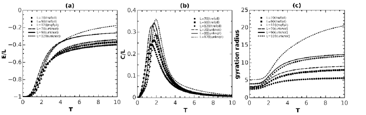
Figure 1: Specific energy, specific heat capacity and gyration radius for the unknot and the trefoil as functions of the temperature. Polymers with lengths $L=70,90$ and $120$ are considered. (a) Plot of the specific energy (in $\varepsilon$-units); (b) Plot of the specific heat capacity (in $\varepsilon$-units); (c) Plot of the radius of gyration.

In Fig. 1 are displayed the results for the unknot and the trefoil. It is found that the growth of the specific energies $\langle E(\beta)\rangle/L$ in Fig. 1(a) is characterised by three regions. At very low temperatures the energy growth is practically zero because the temperatures are too low to allow contacts between the monomers. When the energy is enough to excite more states, the specific energy grows rapidly as a function of the temperature until saturation is reached and the energy increase becomes moderate. The fast increasing energy region causes a peak of the heat capacity as shown in Fig. 1(b) as it has been explained in details in [18]. Concerning the topological effects, we observe that both the energy and the heat capacity grow with growing knot complexity, as it turns out from Fig. 2 by comparing the plots for various knots with the same length $L=90$. Fig. 1(c) shows that in the attractive energy case the mean square gyration radius $\langle R_{G}^{2}\rangle(\beta)$ grows with increasing temperatures. This is an expected behavior. As a matter of fact, in the case of attractive forces the polymer turns out to be in a crumpled conformation at very low temperatures with many contacts in order to minimize the energy. On the contrary, at high temperatures the energy of the thermal fluctuations is large with respect to $\varepsilon$, so that the attractive forces become negligible. Thus, the number of contacts $m$ will be in the average smaller at higher temperatures than at lower energies. As it is intuitive, a smaller number of contacts $m$ corresponds to a larger volume occupied by the knot, which causes the observed increase of the radius of gyration with growing temperatures.

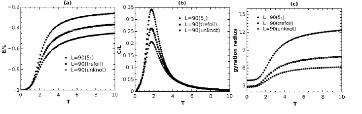
Figure 2: Specific energy and heat capacities as functions of the temperature for the unknot, the trefoil and the knot $5_{1}$ with length $L=90$. (a) Plot of the specific energy (in $\varepsilon$-units); (b) Plot of the specific heat capacity (in $\varepsilon$-units); (c) Plot of the gyration radius.

4 Conclusions

We have studied the thermal properties of a few types of polymer knots using the PAEA algorithm of Ref. [18]. The number of polymer segments affected by the pivot moves has been limited to four. In this case the PAEA method is able to preserve the topology of the knot exactly [18]. The results of [18], which took into account only short-range repulsive forces, have been extended to attractive forces and the calculation of the gyration radius has been added. The thermal properties of the unknot, the knot $3_{1}$ and $5_{1}$ have been analysed with the help of Monte Carlo simulations based on the Wang-Landau algorithm and the pivot method. A brief account about the Wang-Landau method has been provided. The results, including those with the new topology $5_{1}$, confirm those of Ref. [18] even when the interactions are attractive. In particular, the presence of the three regimes of growth of the specific energy mentioned in the previous Section has been observed. Moreover, the role of the topological effects, which make both the energy and the heat capacity increase with increasing knot complexity, is confirmed. The data coming from the calculation of the gyration radius give a measure of the size of the polymer knot at different temperatures. When the temperature is low, the number of contacts is at its maximum and the gyration radius is at its minimum. The size of the polymer points out to a possible crumpled conformation. At high temperatures, the influence of the attractive forces becomes negligible and the gyration radius attains slowly its maximum. Even if we limited ourselves to simple short-range interactions, there are no obstacles to extend our procedure to more realistic polymer systems.

References

- [1] A. Yu. Grosberg Phys.-Usp. 40, 12 (1997).
- [2] W. R. Taylor, Nature (London) 406, 916 (2000).
- [3] V. Katritch, J. Bednar, D. Michoud, R. G. Scharein, J. Dubochet, A. Stasiak, Nature 384, 142 (1996).
- [4] V. Katritch, W. K. Olson, P. Pieranski, J. Dubochet and A. Stasiak, Nature 388, 148 (1997).
- [5] M. A. Krasnow, A. Stasiak, S. J. Spengler, F. Dean, T. Koller and N. R. Cozzarelli, Nature 304, 559 (1983).
- [6] B. Laurie, V. Katritch, J. Dubochet and A. Stasiak, Biophys. Jour. 74, 2815 (1998).
- [7] J. I. Sułkowksa, P. Sułkowksa, P. Szymczak and M. Cieplak, Phys. Rev. Lett. 100, 058106 (2008).
- [8] Z. Liu, E. L. Zechiedrich, and H. S. Chan, Biophys. J. 90, 2344 (2006).
- [9] S. A. Wasserman and N. R. Cozzarelli, Science 232, 951 (1986).
- [10] D. W. Sumners, “Knot theory and DNA,” in New Scientific Applications of Geometry and Topology, edited by D. W. Sumners, Proceedings of Symposia in Applied Mathematics, Vol. 45, ͑American Mathematical Society, Providence, RI, 1992, 39.
- [11] A. V. Vologodski, ̵̆ A. V. Lukashin, M. D. Frank-Kamenetski ̵̆ and V. V. Anshelevich, Zh. Eksp. Teor. Fiz. 66, 2153 (1974); Sov. Phys. JETP 39, 1059 (1975); M. D. Frank-Kamenetskii, A. V. Lukashin and A. V. Vologodskii, Nature (London) 258, 398 (1975).
- [12] E. Orlandini, S. G. Whittington, Rev. Mod. Phys. 79, 611 (2007); C. Micheletti, D. Marenduzzo, and E. Orlandini, Phys. Reports 504, 1 (2011).
- [13] T. Vettorel, A. Yu. Grosberg and K. Kremer, Phys. Biol. 6, 025013 (2009).
- [14] P. Virnau, Y. Kantor and M. Kardar, J. Am. Chem. Soc. 127 (43), 15102 (2005).
- [15] P. Pierański, S. Przybył and A. Stasiak, EPJ E 6 (2), 123 (2001).
- [16] R. Metzler, A. Hanke, P. G. Dommersnes, Y. Kantor and M. Kardar, Phys. Rev. Lett. 88, 188101 (2002).
- [17] K. Koniaris and M. Muthukumar, Phys. Rev. Lett. 66, 2211 (1991).
- [18] Y. Zhao and F. Ferrari, J. Stat. Mech. (2012) P11022.
- [19] A. Swetnam, C. Brett and M. P. Allen, Phys. Rev. E 85, 031804 (2012).
- [20] R. Scharein et. al., J. Phys. A: Math. Gen. 43, 475006 (2009).
- [21] N. Madras, A. Orlistsky and L. A. Shepp, Journal of Statistical Physics 58, 159 (1990).
- [22] F. Wang and D. P. Landau, Phys. Rev. Lett. 86, 2050 (2001).
- [23] N. A. Volkov, A. A. Yurchenko, A. P. Lyubartsev and P. N. Vorontsov-Velyaminov, Macromol. Theory Simul. 14, 491-504 (2005).
- [24] P. N. Vorontsov-Velyaminov, N. A. Volkov, A. A. Yurchenko and A. P. Lyubartsev, Polymer Science, Ser. A 52, 742 (2010).