Alternating Directions Dual Decomposition

Abstract

We propose AD³, a new algorithm for approximate maximum a posteriori (MAP) inference on factor graphs based on the alternating directions method of multipliers. Like dual decomposition algorithms, AD³ uses worker nodes to iteratively solve local subproblems and a controller node to combine these local solutions into a global update. The key characteristic of AD³ is that each local subproblem has a quadratic regularizer, leading to a faster consensus than subgradient-based dual decomposition, both theoretically and in practice. We provide closed-form solutions for these AD³ subproblems for binary pairwise factors and factors imposing first-order logic constraints. For arbitrary factors (large or combinatorial), we introduce an active set method which requires only an oracle for computing a local MAP configuration, making AD³ applicable to a wide range of problems. Experiments on synthetic and real-world problems show that AD³ compares favorably with the state-of-the-art.

1 Introduction

Graphical models enable compact representations of probability distributions, being widely used in computer vision, natural language processing (NLP), and computational biology (Pearl, 1988; Lauritzen, 1996; Koller and Friedman, 2009). When using these models, a central problem is that of inferring the most probable (a.k.a. maximum a posteriori – MAP) configuration. Unfortunately, exact MAP inference is an intractable problem for many graphical models of interest in applications, such as those involving non-local features and/or structural constraints. This fact has motivated a significant research effort on approximate MAP inference.

A class of methods that proved effective for approximate inference is based on linear programming relaxations of the MAP problem (LP-MAP) (Schlesinger, 1976). Several message-passing algorithms have been proposed to address the resulting LP problems, taking advantage of the underlying graph structure (Wainwright et al., 2005; Kolmogorov, 2006; Werner, 2007; Globerson and Jaakkola, 2008; Ravikumar et al., 2010). In the same line, Komodakis et al. (2007) proposed a method based on the classical dual decomposition (Dantzig and Wolfe, 1960; Everett III, 1963; Shor, 1985), which breaks the original problem into a set of smaller subproblems; this set of subproblems, together with the constraints that they should agree on the shared variables, yields a constrained optimization problem, the Lagrange dual of which is solved using a projected subgradient method. Initially proposed for computer vision (Komodakis et al., 2007; Komodakis and Paragios, 2009), this technique has also been shown effective in several NLP tasks that involve combinatorial constraints, such as parsing and machine translation (Koo et al., 2010; Rush et al., 2010; Auli and Lopez, 2011; Rush and Collins, 2011; Chang and Collins, 2011; DeNero and Macherey, 2011). The major drawback is that the subgradient algorithm is very slow to achieve consensus in problems with a large number of overlapping components, requiring $O(1/\epsilon^{2})$ iterations for an $\epsilon$-accurate solution. Jojic et al. (2010) addressed this drawback by introducing an accelerated method that enjoys a faster convergence rate $O(1/\epsilon)$; however, that method is sensitive to previous knowledge of $\epsilon$ and the prescription of a temperature parameter, which may yield numerical instabilities.

In this paper, we ally the simplicity of dual decomposition (DD) with the effectiveness of augmented Lagrangian methods, which have a long-standing history in optimization (Hestenes, 1969; Powell, 1969). In particular, we employ the alternating directions method of multipliers (ADMM), a method introduced in the optimization community in the 1970s (Glowinski and Marroco, 1975; Gabay and Mercier, 1976) which has seen a recent surge of interest in machine learning and signal processing (Afonso et al., 2010; Mota et al., 2010; Goldfarb et al., 2010; Boyd et al., 2011). The result is a new LP-MAP inference algorithm called AD³ (alternating directions dual decomposition), which enjoys $O(1/\epsilon)$ convergence rate. We show that AD³ is able to solve the LP-MAP problem more efficiently than other methods. Like the projected subgradient algorithm of Komodakis et al. (2007), AD³ is an iterative “consensus algorithm,” alternating between a broadcast operation, where subproblems are distributed across local workers, and a gather operation, where the local solutions are assembled by a controller. The key difference is that AD³ also broadcasts the current global solution, allowing the local workers to regularize their subproblems toward that solution. This has the effect of speeding up consensus, without sacrificing the modularity of DD algorithms.

Our main contributions are:

• We derive AD³ and establish its convergence properties, blending classical and newer results about ADMM (Glowinski and Le Tallec, 1989; Eckstein and Bertsekas, 1992; Wang and Banerjee, 2012). We show that the algorithm has the same form as the DD method of Komodakis et al. (2007), with the local MAP subproblems replaced by quadratic programs.

• We show that these AD³ subproblems can be solved exactly and efficiently in many cases of interest, including Ising models and a wide range of hard factors representing arbitrary constraints in first-order logic. Up to a logarithmic term, the asymptotic cost is the same as that of passing messages or doing local MAP inference.

• For factors lacking a closed-form solution of the AD³ subproblems, we introduce a new active set method. Remarkably, our method requires only a black box that returns local MAP configurations for each factor (the same requirement of the projected subgradient algorithm). This paves the way for using AD³ with large dense or structured factors, based on off-the-shelf combinatorial algorithms (e.g., Viterbi, Chu-Liu-Edmonds, Ford-Fulkerson).

• We show that AD³ can be wrapped into a branch-and-bound procedure to retrieve the exact MAP configuration.

AD³ was originally introduced by Martins et al. (2010a, 2011a) (then called DD-ADMM). In addition to a considerably more detailed presentation, this paper contains contributions that substantially extend that preliminary work in several directions: the $O(1/\epsilon)$ rate of convergence, the active set method for general factors, and the branch-and-bound procedure for exact MAP inference. It also reports a wider set of experiments and the release of open-source code (available at http://www.ark.cs.cmu.edu/AD3), which may be useful to other researchers in the field.

This paper is organized as follows. We start by providing background material: MAP inference in graphical models and its LP-MAP relaxation (Section 2); the projected subgradient algorithm for the DD of Komodakis et al. (2007) (Section 3). In Section 4, we derive AD³ and analyze its convergence. The AD³ local subproblems are addressed in Section 5, where closed-form solutions are derived for Ising models and several structural constraint factors. In Section 6, we introduce an active set method to solve the AD³ subproblems for arbitrary factors. Experiments with synthetic models, as well as in protein design and dependency parsing (Section 7) testify for the success of our approach. Finally, related work in discussed in Section 8, and Section 9 concludes the paper.

2 Background

2.1 Factor Graphs

Let $\boldsymbol{Y}:=(Y_{1},\ldots,Y_{M})$ be a tuple of random variables, where each $Y_{i}$ takes values in a finite set ${\mathcal{Y}}_{i}$ and $\boldsymbol{Y}$ takes values in the corresponding Cartesian product set ${\mathcal{Y}}:=\prod_{i=1}^{M}{\mathcal{Y}}_{i}$. Graphical models (e.g., Bayesian networks, Markov random fields) are structural representations of joint probability distributions, which conveniently model statistical (in)dependencies among the variables. In this paper, we focus on factor graphs, introduced by Tanner (1981) and Kschischang et al. (2001).

Definition 1 (Factor graph.)

A factor graph is a bipartite graph $\mathscr{G}:=(\mathcal{V},\mathcal{F},\mathcal{E})$, comprised of:

• a set of variable nodes $\mathcal{V}:=\{1,\ldots,M\}$, corresponding to the variables $(Y_{1},\ldots,Y_{M})$;

• a set of factor nodes $\mathcal{F}$ (disjoint from $\mathcal{V}$);

• a set of edges $\mathcal{E}\subseteq\mathcal{V}\times\mathcal{F}$ linking variable nodes to factor nodes.

For notational convenience, we use Latin letters ($i,j,...$) and Greek letters ($\alpha,\beta,...$) to refer to variable and factor nodes, respectively. We denote by $\mathcal{N}(\cdot)$ the neighborhood set of its node argument, whose cardinality is called the degree of the node. Formally, $\mathcal{N}(i):=\{\alpha\in\mathcal{F}\,\,|\,\,(i,\alpha)\in\mathcal{E}\}$, for variable nodes, and $\mathcal{N}(\alpha):=\{i\in\mathcal{V}\,\,|\,\,(i,\alpha)\in\mathcal{E}\}$ for factor nodes. We use the short notation $\boldsymbol{Y}_{\!\!\alpha}$ to denote the tuple of variables linked to factor $\alpha$, i.e., $\boldsymbol{Y}_{\!\!\alpha}:=(Y_{i})_{i\in\mathcal{N}(\alpha)}$, and lowercase to denote instantiations of random variables, e.g., $Y_{i}=y_{i}$ and $\boldsymbol{Y}_{\!\!\alpha}=\boldsymbol{y}_{\alpha}$.

The joint probability distribution of $(Y_{1},\ldots,Y_{M})$ is said to factor according to the factor graph $\mathscr{G}=(\mathcal{V},\mathcal{F},\mathcal{E})$ if it can be written as

$$\mathbb{P}(Y_{1}=y_{1},\ldots,Y_{M}=y_{M})\,\,\propto\,\,\exp\left(\sum_{i\in\mathcal{V}}{\theta}_{i}(y_{i})+\sum_{\alpha\in\mathcal{F}}{\theta}_{\alpha}(\boldsymbol{y}_{\alpha})\right),$$ (1)

where ${\theta}_{i}(\cdot)$ and ${\theta}_{\alpha}(\cdot)$ are called, respectively, the unary and higher-order log-potential functions. To accommodate hard constraints, we allow these functions to take values in $\mathbb{R}\cup\{-\infty\}$. Fig. 1 shows examples of factor graphs with hard constraint factors (to be studied in detail in Section 5.3). For notational convenience, we represent potential functions as vectors, $\boldsymbol{\theta}_{i}:=({\theta}_{i}(y_{i}))_{y_{i}\in{\mathcal{Y}}_{i}}$ and $\boldsymbol{\theta}_{\alpha}:=({\theta}_{\alpha}(\boldsymbol{y}_{\alpha}))_{\boldsymbol{y}_{\alpha}\in{\mathcal{Y}}_{\alpha}}$, where ${\mathcal{Y}}_{\alpha}=\prod_{i\in\mathcal{N}(\alpha)}{\mathcal{Y}}_{i}$. We denote by $\boldsymbol{\theta}$ the vector of dimension $\sum_{i\in\mathcal{V}}|{\mathcal{Y}}_{i}|+\sum_{\alpha\in\mathcal{F}}|{\mathcal{Y}}_{\alpha}|$ obtained by stacking all these vectors.

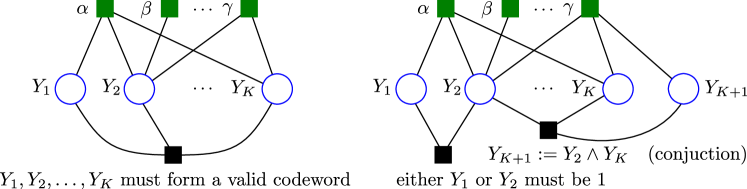
Figure 1: Constrained factor graphs, with soft factors shown as green squares above the variable nodes (circles) and hard constraint factors as black squares below the variable nodes. Left: a global factor that constrains the set of admissible outputs to a given codebook. Right: examples of declarative constraints; one of them is a factor connecting existing variables to an extra variable, allows scores depending on a logical functions of the former.

2.2 MAP Inference

Given a factor graph $\mathscr{G}$, along with all the log-potential functions—which fully specify the joint distribution of $Y_{1},\ldots,Y_{M}$—we are interested in finding an assignment with maximal probability (the so-called MAP assignment/configuration):

$${\widehat{\boldsymbol{y}}} \in \arg\max_{y_{1},\ldots,y_{M}}\mathbb{P}(Y_{1}=y_{1},\ldots,Y_{M}=y_{M})$$ (2)

$$= \arg\max_{y_{1},\ldots,y_{M}}\sum_{\alpha\in\mathcal{F}}{\theta}_{\alpha}(\boldsymbol{y}_{\alpha})+\sum_{i\in\mathcal{V}}{\theta}_{i}(y_{i}).$$

This combinatorial problem, which is NP-hard in general (Koller and Friedman, 2009), can be transformed into a linear program by using the concept of marginal polytope (Wainwright and Jordan, 2008), as next described. Let $\Delta^{K}$ denote the $K$-dimensional probability simplex,

$$\Delta^{K}:=\{\boldsymbol{u}\in\mathbb{R}^{K}\,\,|\,\,\boldsymbol{u}\geq\mathbf{0},\,\,{\mathbf{1}}^{\top}{\boldsymbol{u}}=1\}=\operatorname{conv}\{\boldsymbol{e}_{1},\ldots,\boldsymbol{e}_{K}\},$$ (3)

where $\boldsymbol{e}_{j}$ has all entries equal to zero except for the $j$th one, which is equal to one. We introduce “local” probability distributions over the variables and factors, $\boldsymbol{p}_{i}\in\Delta^{|{\mathcal{Y}}_{i}|}$ and $\boldsymbol{q}_{\alpha}\in\Delta^{|{\mathcal{Y}}_{\alpha}|}$. We stack these distributions into vectors $\boldsymbol{p}$ and $\boldsymbol{q}$, with dimensions $P:=\sum_{i\in\mathcal{V}}|{\mathcal{Y}}_{i}|$ and $Q:=\sum_{\alpha\in\mathcal{F}}|{\mathcal{Y}}_{\alpha}|$, respectively, and denote by $(\boldsymbol{p},\boldsymbol{q})\in\mathbb{R}^{P+Q}$ their concatenation. We say that $(\boldsymbol{p},\boldsymbol{q})$ is globally consistent if the local distributions $\{\boldsymbol{p}_{i}\}$ and $\{\boldsymbol{q}_{\alpha}\}$ are the marginals of some global joint distribution. The set of all globally consistent vectors $(\boldsymbol{p},\boldsymbol{q})$ is called the marginal polytope of $\mathscr{G}$, denoted as $\mathrm{MARG}(\mathscr{G})$. There is a one-to-one mapping between the vertices of $\mathrm{MARG}(\mathscr{G})$ and the set of possible configurations $\mathcal{Y}$: each $\boldsymbol{y}\in\mathcal{Y}$ corresponds to a vertex $(\boldsymbol{p},\boldsymbol{q})$ of $\mathrm{MARG}(\mathscr{G})$ consisting of “degenerate” distributions $\boldsymbol{p}_{i}=\boldsymbol{e}_{y_{i}}$ and $\boldsymbol{q}_{\alpha}=\boldsymbol{e}_{\boldsymbol{y}_{\alpha}}$, for each $i\in\mathcal{V}$ and $\alpha\in\mathcal{F}$. The MAP problem in (2) is then equivalent to the following linear program (LP):

$$\boxed{\begin{array}[]{lll}\textbf{MAP:}&\mathrm{maximize}&\displaystyle\sum_{\alpha\in\mathcal{F}}{\boldsymbol{\theta}_{\alpha}}^{\top}{\boldsymbol{q}_{\alpha}}+\sum_{i\in\mathcal{V}}{\boldsymbol{\theta}_{i}}^{\top}{\boldsymbol{p}_{i}}\\ &\text{with respect to}&(\boldsymbol{p},\boldsymbol{q})\in\mathrm{MARG}(\mathscr{G}).\end{array}}$$ (4)

The equivalence between (2) and (4) stems from the fact that any linear program on a bounded convex constraint polytope attains a solution at a vertex of that polytope (see, e.g., Rockafellar (1970)). Unfortunately, the linear program (4) is not easier to solve than (2): for a graph $\mathscr{G}$ with cycles (which induce global consistency constraints that are hard to specify concisely), the number of linear inequalities that characterize $\mathrm{MARG}(\mathscr{G})$ may grow superpolynomially with the size of $\mathscr{G}$. As a consequence, approximations of $\mathrm{MARG}(\mathscr{G})$ have been actively investigated in recent years.

2.3 LP-MAP Inference

Tractable approximations of $\mathrm{MARG}(\mathscr{G})$ can be built by using weaker constraints that all realizable marginals must satisfy to ensure local consistency:

1. Non-negativity: all local marginals $p_{i}(y_{i})$ and $q_{\alpha}(\boldsymbol{y}_{\alpha})$ must be non-negative.

2. Normalization: local marginals must be properly normalized, i.e., $\sum_{y_{i}\in{\mathcal{Y}}_{i}}p_{i}(y_{i})=1$, for all $i\in\mathcal{V}$, and $\sum_{\boldsymbol{y}_{\alpha}\in{\mathcal{Y}}_{\alpha}}q_{\alpha}(\boldsymbol{y}_{\alpha})=1$, for all $\alpha\in\mathcal{F}$.

3. Marginalization: a variable participating in a factor must have a marginal which is consistent with the factor marginals, i.e., $p_{i}(y_{i})=\sum_{\boldsymbol{y}_{\alpha}\sim y_{i}}q_{\alpha}(\boldsymbol{y}_{\alpha})$, for all $(i,\alpha)\in\mathcal{E}$ and $y_{i}\in{\mathcal{Y}}_{i}$.

Note that some of these constraints are redundant: the non-negativity of $q_{\alpha}(\boldsymbol{y}_{\alpha})$ and the marginalization constraint imply the non-negativity of $p_{i}(y_{i})$; the normalization of $\boldsymbol{q}_{\alpha}$ and the marginalization constraints imply $\sum_{y_{i}\in{\mathcal{Y}}_{i}}p_{i}(y_{i})=1$. For convenience, we express those constraints in vector notation. For each $(i,\alpha)\in\mathcal{E}$, we define a (consistency) matrix $\mathbf{M}_{i\alpha}\in\mathbb{R}^{|\mathcal{Y}_{i}|\times|\mathcal{Y}_{\alpha}|}$ as follows:

$$\mathbf{M}_{i\alpha}(y_{i},\boldsymbol{y}_{\alpha})=\left\{\begin{array}[]{ll}1,&\text{if $\boldsymbol{y}_{\alpha}\sim y_{i}$}\\ 0,&\text{otherwise.}\end{array}\right.$$ (5)

The local marginalization constraints can be expressed as $\mathbf{M}_{i\alpha}\boldsymbol{q}_{\alpha}=\boldsymbol{p}_{i}.$ Combining all the local consistency constraints, and dropping redundant ones, yields the so-called local polytope:

$$\mathrm{LOCAL}(\mathscr{G})=\left\{(\boldsymbol{p},\boldsymbol{q})\in\mathbb{R}^{P+Q}\,\,\Bigg{|}\,\,\begin{array}[]{ll}\boldsymbol{q}_{\alpha}\in\Delta^{|{\mathcal{Y}}_{\alpha}|},&\forall\alpha\in\mathcal{F}\\ \mathbf{M}_{i\alpha}\boldsymbol{q}_{\alpha}=\boldsymbol{p}_{i},&\forall(i,\alpha)\in\mathcal{E}\\ \end{array}\right\}.$$ (6)

The number of constraints that define $\mathrm{LOCAL}(\mathscr{G})$ grows linearly with $P+Q$, rather than superpolynomially. The elements of $\mathrm{LOCAL}(\mathscr{G})$ are called pseudo-marginals. Since any true marginal vector must satisfy the constraints above, $\mathrm{LOCAL}(\mathscr{G})$ is an outer approximation, i.e.,

$$\mathrm{MARG}(\mathscr{G})\subseteq\mathrm{LOCAL}(\mathscr{G}),$$ (7)

as illustrated in Fig. 2.

Figure 2: Marginal polytope (in green) and its outer aproximation, the local polytope (in blue). Each element of the marginal polytope corresponds to a joint distribution of $Y_{1},\ldots,Y_{M}$, and each vertex corresponds to a configuration $\boldsymbol{y}\in\mathcal{Y}$, having coordinates in $\{0,1\}$. The local polytope may have additional fractional vertices, with coordinates in $[0,1]$.

This approximation is tight for tree-structured graphs and other special cases, but not in general (even for small graphs with cycles) (Wainwright and Jordan, 2008). The LP-MAP problem results from replacing $\mathrm{MARG}(\mathscr{G})$ by $\mathrm{LOCAL}(\mathscr{G})$ in (4) (Schlesinger, 1976):

$$\boxed{\begin{array}[]{lll}\textbf{LP-MAP:}&\mathrm{maximize}&\displaystyle\sum_{\alpha\in\mathcal{F}}{\boldsymbol{\theta}_{\alpha}}^{\top}{\boldsymbol{q}_{\alpha}}+\sum_{i\in\mathcal{V}}{\boldsymbol{\theta}_{i}}^{\top}{\boldsymbol{p}_{i}}\\ &\text{with respect to}&(\boldsymbol{p},\boldsymbol{q})\in\mathrm{LOCAL}(\mathscr{G}).\end{array}}$$ (8)

It can be shown that the points of $\mathrm{LOCAL}(\mathscr{G})$ that are integer are the vertices of $\mathrm{MARG}(\mathscr{G})$; therefore, the solution of LP-MAP provides an upper bound on the optimal objective of MAP.

2.4 LP-MAP Inference Algorithms

While any off-the-shelf LP solver can be used for solving (8), specialized algorithms have been designed to exploit the graph structure, achieving superior performance on several benchmarks (Yanover et al., 2006). Most of these specialized algorithms belong to two classes: block (dual) coordinate descent, which take the form of message-passing algorithms, and projected subgradient algorithms, based on dual decomposition.

Block coordinate descent methods address the dual of (8) by alternately optimizing over blocks of coordinates. Different choices of blocks lead to different algorithms: max-sum diffusion (Kovalevsky and Koval, 1975; Werner, 2007); max-product sequential tree-reweighted belief propagation (TRW-S) (Wainwright et al., 2005; Kolmogorov, 2006); max-product linear programming (MPLP) (Globerson and Jaakkola, 2008). These algorithms work by passing messages (that require computing max-marginals) between factors and variables. Under certain conditions, if the relaxation is tight, one may obtain optimality certificates. If the relaxation is not tight, it is sometimes possible to reduce the problem size or use a cutting-plane method to move toward the exact MAP (Sontag et al., 2008). A disadvantage of block coordinate descent algorithms is that they may stop at suboptimal solutions, since the objective is non-smooth (Bertsekas et al. 1999, Section 6.3.4).

Projected subgradient based on the dual decomposition is a classical technique (Dantzig and Wolfe, 1960; Everett III, 1963; Shor, 1985), which was first proposed in the context of graphical models by Komodakis et al. (2007) and Johnson et al. (2007). Due to its strong relationship with the approach pursued in this paper, that method is described in detail in the next section.

3 Dual Decomposition with the Projected Subgradient Algorithm

The projected subgradient method for dual decomposition can be seen as an iterative “consensus algorithm,” alternating between a broadcast operation, where local subproblems are distributed across worker nodes, and a gather operation, where the local solutions are assembled by a master node to update the current global solution. At each round, the worker nodes perform local MAP inference independently; hence, the algorithm is completely modular and trivially parallelizable.

For each edge $(i,\alpha)\in\mathcal{E}$, define a potential function $\boldsymbol{\theta}_{i\alpha}:=({\theta}_{i\alpha}(y_{i}))_{y_{i}\in{\mathcal{Y}}_{i}}$ that satisfies $\sum_{\alpha\in\mathcal{N}(i)}\boldsymbol{\theta}_{i\alpha}=\boldsymbol{\theta}_{i}$; a trivial choice is $\boldsymbol{\theta}_{i\alpha}=|\mathcal{N}(i)|^{-1}\boldsymbol{\theta}_{i}$. The objective (8) can be rewritten as

$$\sum_{\alpha\in\mathcal{F}}{\boldsymbol{\theta}_{\alpha}}^{\top}{\boldsymbol{q}_{\alpha}}+\sum_{i\in\mathcal{V}}{\boldsymbol{\theta}_{i}}^{\top}{\boldsymbol{p}_{i}} = \sum_{\alpha\in\mathcal{F}}{\left({\boldsymbol{\theta}}_{\alpha}+\sum_{i\in\mathcal{N}(\alpha)}\mathbf{M}_{i\alpha}^{\top}\boldsymbol{\theta}_{i\alpha}\right)}^{\top}{\boldsymbol{q}_{\alpha}},$$ (9)

because $\boldsymbol{p}_{i}=\mathbf{M}_{i\alpha}\boldsymbol{q}_{\alpha}$. The LP-MAP problem (8) is then equivalent to the following primal formulation, which we call LP-MAP-P:

$$\boxed{\begin{aligned} \textbf{LP-MAP-P:}\qquad\mathrm{maximize}\quad&\sum_{\alpha\in\mathcal{F}}{\left({\boldsymbol{\theta}}_{\alpha}+\sum_{i\in\mathcal{N}(\alpha)}\mathbf{M}_{i\alpha}^{\top}\boldsymbol{\theta}_{i\alpha}\right)}^{\top}{\boldsymbol{q}_{\alpha}}\\ \text{with respect to}\quad&\boldsymbol{q}_{\alpha}\in\Delta^{|{\mathcal{Y}}_{\alpha}|},\forall\alpha\in\mathcal{F},\\ &\boldsymbol{p}\in\mathbb{R}^{P},\\ \text{subject to}\quad&\mathbf{M}_{i\alpha}\boldsymbol{q}_{\alpha}=\boldsymbol{p}_{i},\,\,\forall(i,\alpha)\in\mathcal{E}.\end{aligned}}$$ (10)

Note that, although the $\boldsymbol{p}$-variables do not appear in the objective of (10), they play a fundamental role through the constraints in the last line, which are necessary to ensure that the marginals encoded in the $\boldsymbol{q}$-variables are consistent on their overlaps. Indeed, it is this set of constraints that complicate the optimization problem, which would otherwise be separable into independent subproblems, one per factor. Introducing a Lagrange multiplier ${\lambda}_{i\alpha}(y_{i})$ for each of these equality constraints leads to the Lagrangian function

$$L(\boldsymbol{q},\boldsymbol{p},\boldsymbol{\lambda}) = \sum_{\alpha\in\mathcal{F}}{\left({\boldsymbol{\theta}}_{\alpha}+\sum_{i\in\mathcal{N}(\alpha)}\mathbf{M}_{i\alpha}^{\top}(\boldsymbol{\theta}_{i\alpha}+\boldsymbol{\lambda}_{i\alpha})\right)}^{\top}{\boldsymbol{q}_{\alpha}}-\sum_{(i,\alpha)\in\mathcal{E}}{\boldsymbol{\lambda}_{i\alpha}}^{\top}{\boldsymbol{p}_{i}},$$ (11)

the maximization of which w.r.t. $\boldsymbol{q}$ and $\boldsymbol{p}$ will yield the (Lagrangian) dual objective. Since the $\boldsymbol{p}$-variables are unconstrained, we have

$$\max_{\boldsymbol{q},\boldsymbol{p}}L(\boldsymbol{q},\boldsymbol{p},\boldsymbol{\lambda})=\left\{\begin{array}[]{ll}\displaystyle g(\boldsymbol{\lambda})&\text{if $\boldsymbol{\lambda}\in\Lambda$,}\\ +\infty&\text{otherwise,}\end{array}\right.$$ (14)

where $g(\boldsymbol{\lambda})=\sum_{\alpha\in\mathcal{F}}g_{\alpha}(\boldsymbol{\lambda})$ is the dual objective function,

$$\Lambda:=\left\{\boldsymbol{\lambda}\,\,\bigg{|}\,\,\sum_{\alpha\in\mathcal{N}(i)}\boldsymbol{\lambda}_{i\alpha}=\mathbf{0},\,\,\forall i\in\mathcal{V}\right\},$$ (15)

and each $g_{\alpha}(\boldsymbol{\lambda})$ is the solution of a local problem (called the $\alpha$-subproblem):

$$g_{\alpha}(\boldsymbol{\lambda}) := \max_{\boldsymbol{q}_{\alpha}\in\Delta^{|{\mathcal{Y}}_{\alpha}|}}{\left({\boldsymbol{\theta}}_{\alpha}+\sum_{i\in\mathcal{N}(\alpha)}\mathbf{M}_{i\alpha}^{\top}(\boldsymbol{\theta}_{i\alpha}+\boldsymbol{\lambda}_{i\alpha})\right)}^{\top}{\boldsymbol{q}_{\alpha}}$$ (16)

$$= \max_{\boldsymbol{y}_{\alpha}\in{\mathcal{Y}}_{\alpha}}\left({\theta}_{\alpha}(\boldsymbol{y}_{\alpha})+\sum_{i\in\mathcal{N}(\alpha)}({\theta}_{i\alpha}(y_{i})+\lambda_{i\alpha}(y_{i}))\right);$$ (17)

the last equality is justified by the fact that maximizing a linear objective over the probability simplex gives the largest component of the score vector. Finally, the dual problem is

$$\boxed{\begin{array}[]{lll}\textbf{LP-MAP-D:}&\mathrm{minimize}&\displaystyle g(\boldsymbol{\lambda})\\ &\text{with respect to}&\boldsymbol{\lambda}\in\Lambda.\end{array}}$$ (18)

Problem (18) is often referred to as the master or controller, and each $\alpha$-subproblem (16)–(17) as a slave or worker. Note that each of these $\alpha$-subproblems is itself a local MAP problem, involving only factor $\alpha$. As a consequence, the solution $\widehat{\boldsymbol{q}}_{\alpha}$ of (16) is an indicator vector corresponding to a particular configuration $\widehat{\boldsymbol{y}}_{\alpha}$ (the solution of (17) ), that is, $\widehat{\boldsymbol{q}}_{\alpha}=\boldsymbol{e}_{\widehat{\boldsymbol{y}}_{\alpha}}$.

The dual problem (18) can be solved with a projected subgradient algorithm. By Danskin’s rule (Bertsekas et al., 1999, p. 717), a subgradient of $g_{\alpha}$ is readily given by

$$\frac{\partial g_{\alpha}(\boldsymbol{\lambda})}{\partial\boldsymbol{\lambda}_{i\alpha}}=\mathbf{M}_{i\alpha}\widehat{\boldsymbol{q}}_{\alpha}:=\widehat{\boldsymbol{q}}_{i\alpha},\quad\forall(i,\alpha)\in\mathcal{E};$$ (19)

and the projection onto $\Lambda$ amounts to a centering operation. The $\alpha$-subproblems (16)–(17) can be handled in parallel and then have their solutions gathered for computing this projection and update the Lagrange variables. Putting these pieces together yields Algorithm 1, which assumes a black-box procedure ComputeMap that returns a local MAP assignment (as an indicator vector), given log-potentials as input. At each iteration, the algorithm broadcasts the current Lagrange multipliers to all the factors. Each factor adjusts its internal unary log-potentials (line 6) and invokes the ComputeMap procedure (line 7). The solutions achieved by each factor are then gathered and averaged (line 10), and the Lagrange multipliers are updated with step size $\eta_{t}$ (line 11). The two following propositions establish the convergence properties of Algorithm 1.

Algorithm 1 Dual Decomposition with Projected Subgradient (Komodakis et al., 2007)

1:  input: graph $\mathscr{G}$, parameters $\boldsymbol{\theta}$, maximum number of iterations $T$, stepsizes $(\eta_{t})_{t=1}^{T}$

2:  for each $(i,\alpha)\in\mathcal{E}$, choose $\boldsymbol{\theta}_{i\alpha}$ such that $\sum_{\alpha\in\mathcal{N}(i)}\boldsymbol{\theta}_{i\alpha}=\boldsymbol{\theta}_{i}$

3:  initialize $\boldsymbol{\lambda}=\mathbf{0}$

4:  for $t=1$ to $T$ do

5:     for  each factor $\alpha\in\mathcal{F}$ do

6:        set unary log-potentials ${\boldsymbol{\xi}}_{i\alpha}:={\boldsymbol{\theta}}_{i\alpha}+\boldsymbol{\lambda}_{i\alpha}$, for $i\in\mathcal{N}(\alpha)$

7:        set $\widehat{\boldsymbol{q}}_{\alpha}:=\text{\sc ComputeMap}({\boldsymbol{\theta}}_{\alpha}+\sum_{i\in\mathcal{N}(\alpha)}\mathbf{M}_{i\alpha}^{\top}\boldsymbol{\xi}_{i\alpha})$

8:        set $\widehat{\boldsymbol{q}}_{i\alpha}:=\mathbf{M}_{i\alpha}\widehat{\boldsymbol{q}}_{\alpha}$, for $i\in\mathcal{N}(\alpha)$

9:     end for

10:     compute average ${\boldsymbol{p}}_{i}:=|\mathcal{N}(i)|^{-1}\sum_{\alpha\in\mathcal{N}(i)}\widehat{\boldsymbol{q}}_{i\alpha}$ for each $i\in\mathcal{V}$

11:     update $\boldsymbol{\lambda}_{i\alpha}:=\boldsymbol{\lambda}_{i\alpha}-\eta_{t}\left(\widehat{\boldsymbol{q}}_{i\alpha}-{\boldsymbol{p}}_{i}\right)$ for each $(i,\alpha)\in\mathcal{E}$

12:  end for

13:  output: dual variable $\boldsymbol{\lambda}$ and upper bound $g(\boldsymbol{\lambda})$

Proposition 2 (Convergence rate)

Let the non-negative step size sequence $(\eta_{t})_{t\in\mathbb{N}}$ be diminishing and nonsummable: $\lim\eta_{t}=0$ and $\sum_{t=1}^{\infty}\eta_{t}=\infty$. Then, Algorithm 1 converges to the solution of LP-MAP-D (18). Furthermore, $T=O(1/\epsilon^{2})$ iterations of Algorithm 1 are sufficient to achieve a dual objective which differs by $\epsilon$ from the optimal value.

Proof: This is a property of projected subgradient algorithms (see, e.g., Bertsekas et al. 1999).   

Proposition 3 (Certificate of optimality)

If, at some iteration of Algorithm 1, all the local subproblems are in agreement (i.e., if $\widehat{\boldsymbol{q}}_{i\alpha}=\boldsymbol{p}_{i}$ after line 10, for all $i\in\mathcal{V}$), then:

• $\boldsymbol{\lambda}$ is a solution of LP-MAP-D (18);

• $\boldsymbol{p}$ is binary-valued and a solution of both LP-MAP-P and MAP.

Proof: If all local subproblems are in agreement, then a vacuous update will occur in line 11, and no further changes will occur. Since the algorithm is guaranteed to converge, the current $\boldsymbol{\lambda}$ is optimal. Also, if all local subproblems are in agreement, the averaging in line 10 necessarily yields a binary vector $\boldsymbol{p}$. Since any binary solution of LP-MAP is also a solution of MAP, the result follows.   

Propositions 2–3 imply that, if the parameters $\boldsymbol{\theta}$ are such that LP-MAP is a tight relaxation, then Algorithm 1 yields the exact MAP configuration along with a certificate of optimality. According to Proposition 2, even if the relaxation is not tight, Algorithm 1 still converges to a solution of LP-MAP. In some problem domains, the LP-MAP is often tight (Koo and Collins, 2010; Rush et al., 2010); for problems with a relaxation gap, techniques to tighten the relaxation have been developed (Rush and Collins, 2011). However, in large graphs with many overlapping factors, it has been observed that Algorithm 1 can converge quite slowly in practice (Martins et al., 2011b). This is not surprising, given that it attempts to reach a consensus among all overlapping components; the larger this number, the harder it is to achieve consensus. In the next section, we propose a new LP-MAP inference algorithm that is more suitable for this class of problems.

4 Alternating Directions Dual Decomposition (AD³)

4.1 Addressing the Weaknesses of Dual Decomposition with Projected Subgradient

The main weaknesses of Algorithm 1 reside in the following two aspects.

1. The dual objective function $g(\boldsymbol{\lambda})$ is non-smooth, this being why “subgradients” are used instead of “gradients.” It is well-known that non-smooth optimization lacks some of the good properties of its smooth counterpart. Namely, there is no guarantee of monotonic improvement in the objective (see Bertsekas et al. 1999, p. 611). Ensuring convergence requires using a diminishing step size sequence, which leads to slow convergence rates. In fact, as stated in Proposition 2, $O(1/\epsilon^{2})$ iterations are required to guarantee $\epsilon$-accuracy.

2. A close look at Algorithm 1 reveals that the consensus is promoted solely by the Lagrange multipliers (line 6). In a economic interpretation, these represent “price adjustments” that lead to a reallocation of resources. However, no “memory” exists about past allocations or adjustments, so the workers never know how far they are from consensus. It is thus conceivable that a smart use of these quantities could accelerate convergence.

To obviate the first of these problems, Johnson et al. (2007) proposed smoothing the objective function through an “entropic” perturbation (controlled by a “temperature” parameter), which boils down to replacing the $\max$ in (18) by a “soft-max.” As a result, all the local subproblems become marginal (rather than MAP) computations. A related and asymptotically faster method was proposed later by Jojic et al. (2010), who address the resulting smooth optimization problem with an accelerated gradient method (Nesterov, 1983, 2005). That approach guarantees an $\epsilon$-accurate solution after $O(1/\epsilon)$ iterations, an improvement over the $O(1/\epsilon^{2})$ bound of Algorithm 1. However, those methods have some drawbacks. First, they need to operate at near-zero temperatures; e.g., the $O(1/\epsilon)$ iteration bound of Jojic et al. (2010) requires setting the temperature to $O(\epsilon)$, which scales the potentials by $O(1/\epsilon)$ and may lead to numerical instabilities in some problems. Second, the solution of the local subproblems are always dense; although some marginal values may be low, they are never exactly zero. This contrasts with the projected subgradient algorithm, for which the solutions of the local subproblems are MAP configurations. These configurations can be cached across iterations, leading to important speedups (Koo et al., 2010).

We will show that AD³ also yields a $O(1/\epsilon)$ iteration bound without suffering from the two drawbacks above. Unlike Algorithm 1, AD³ broadcasts the current global solution to the workers, thus allowing them to regularize their subproblems toward that solution. This promotes a faster consensus, without sacrificing the modularity of dual decomposition. Another advantage of AD³ is that it keeps track of primal and dual residuals, allowing monitoring the LP-MAP optimization process and stopping when a desired accuracy level is attained.

4.2 Augmented Lagrangians and the Alternating Directions Method of Multipliers

Let us start with a brief overview of augmented Lagrangian methods. Consider the following general convex optimization problem with equality constraints:

$$\begin{array}[]{ll}\mathrm{maximize}&f_{1}(\boldsymbol{q})+f_{2}(\boldsymbol{p})\\ \text{with respect to}&\boldsymbol{q}\in\mathcal{Q},\boldsymbol{p}\in\mathcal{P}\\ \text{subject to}&\mathbf{A}\boldsymbol{q}+\mathbf{B}\boldsymbol{p}=\boldsymbol{c},\end{array}$$ (20)

where $\mathcal{Q}\subseteq\mathbb{R}^{P}$ and $\mathcal{P}\subseteq\mathbb{R}^{Q}$ are convex sets and $f_{1}:\mathcal{Q}\rightarrow\mathbb{R}\cup\{-\infty\}$ and $f_{2}:\mathcal{P}\rightarrow\mathbb{R}\cup\{-\infty\}$ are concave functions. Note that the LP-MAP problem stated in (10) has this form. For any $\eta\geq 0$, consider the problem

$$\begin{array}[]{ll}\mathrm{maximize}&f_{1}(\boldsymbol{q})+f_{2}(\boldsymbol{p})-\frac{\eta}{2}\|\mathbf{A}\boldsymbol{q}+\mathbf{B}\boldsymbol{p}-\boldsymbol{c}\|^{2}\\ \text{with respect to}&\boldsymbol{q}\in\mathcal{Q},\boldsymbol{p}\in\mathcal{P}\\ \text{subject to}&\mathbf{A}\boldsymbol{q}+\mathbf{B}\boldsymbol{p}=\boldsymbol{c},\end{array}$$ (21)

which differs from (20) in the extra term penalizing violations of the equality constraints; since this term vanishes at feasibility, the two problems have the same solution. The reason to consider (21) is that its objective is $\eta$-strongly concave, even if $f_{1}+f_{2}$ is not. The Lagrangian of problem (21),

$$L_{\eta}(\boldsymbol{q},\boldsymbol{p},\boldsymbol{\lambda})=f_{1}(\boldsymbol{q})+f_{2}(\boldsymbol{p})+{\boldsymbol{\lambda}}^{\top}{(\mathbf{A}\boldsymbol{q}+\mathbf{B}\boldsymbol{p}-\boldsymbol{c})}-\frac{\eta}{2}\|\mathbf{A}\boldsymbol{q}+\mathbf{B}\boldsymbol{p}-\boldsymbol{c}\|^{2},$$ (22)

is the $\eta$-augmented Lagrangian of problem (20). The so-called augmented Lagrangian (AL) methods (Bertsekas et al., 1999, Section 4.2) address problem (20) by seeking a saddle point of $L_{\eta_{t}}$, for some sequence $(\eta_{t})_{t\in\mathbb{N}}$. The earliest instance is the method of multipliers (MM) (Hestenes, 1969; Powell, 1969), which alternates between a joint update of $\boldsymbol{q}$ and $\boldsymbol{p}$ through

$$(\boldsymbol{q}^{t+1},\boldsymbol{p}^{t+1}) := \arg\max_{\boldsymbol{q},\boldsymbol{p}}\{L_{\eta_{t}}(\boldsymbol{q},\boldsymbol{p},\boldsymbol{\lambda}^{t})\,\,|\,\,\boldsymbol{q}\in\mathcal{Q},\boldsymbol{p}\in\mathcal{P}\}$$ (23)

and a gradient update of the Lagrange multiplier,

$$\boldsymbol{\lambda}^{t+1} := \boldsymbol{\lambda}^{t}-\eta_{t}(\mathbf{A}\boldsymbol{q}^{t+1}+\mathbf{B}\boldsymbol{p}^{t+1}-\boldsymbol{c}).$$ (24)

Under some conditions, this method is convergent, and even superlinear, if the sequence $(\eta_{t})_{t\in\mathbb{N}}$ is increasing (Bertsekas et al. 1999, Section 4.2). A shortcoming of the MM is that problem (23) may be difficult, since the penalty term of the augmented Lagrangian couples the variables $\boldsymbol{p}$ and $\boldsymbol{q}$. The alternating directions method of multipliers (ADMM) avoids this shortcoming, by replacing the joint optimization (23) by a single block Gauss-Seidel-type step:

$$\boldsymbol{q}^{t+1}:=\arg\max_{\boldsymbol{q}\in\mathcal{Q}}L_{\eta_{t}}(\boldsymbol{q},\boldsymbol{p}^{t},\boldsymbol{\lambda}^{t})=\arg\max_{\boldsymbol{q}\in\mathcal{Q}}f_{1}(\boldsymbol{q})+{(\mathbf{A}^{\top}\boldsymbol{\lambda}^{t})}^{\top}{\boldsymbol{q}}-\frac{\eta_{t}}{2}\|\mathbf{A}\boldsymbol{q}+\mathbf{B}\boldsymbol{p}^{t}-\boldsymbol{c}\|^{2},$$ (25)

$$\boldsymbol{p}^{t+1}:=\arg\max_{\boldsymbol{p}\in\mathcal{P}}L_{\eta_{t}}(\boldsymbol{q}^{t+1},\boldsymbol{p},\boldsymbol{\lambda}^{t})=\arg\max_{\boldsymbol{p}\in\mathcal{P}}f_{2}(\boldsymbol{p})+{(\mathbf{B}^{\top}\boldsymbol{\lambda}^{t})}^{\top}{\boldsymbol{p}}-\frac{\eta_{t}}{2}\|\mathbf{A}\boldsymbol{q}^{t+1}+\mathbf{B}\boldsymbol{p}-\boldsymbol{c}\|^{2}.$$ (26)

In general, problems (25)–(26) are simpler than the joint maximization in (23). ADMM was proposed by Glowinski and Marroco (1975) and Gabay and Mercier (1976) and is related to other optimization methods, such as Douglas-Rachford splitting (Eckstein and Bertsekas, 1992) and proximal point methods (see Boyd et al. 2011 for an historical overview).

4.3 Derivation of AD³

The LP-MAP-P problem (10) can be cast into the form (20) by proceeding as follows:

• let $\mathcal{Q}$ in (20) be the Cartesian product of simplices, $\mathcal{Q}:=\prod_{\alpha\in\mathcal{F}}\Delta^{|{\mathcal{Y}}_{\alpha}|}$, and $\mathcal{P}:=\mathbb{R}^{P}$;

• let $f_{1}(\boldsymbol{q}):=\sum_{\alpha\in\mathcal{F}}{\left({\boldsymbol{\theta}}_{\alpha}+\sum_{i\in\mathcal{N}(\alpha)}\mathbf{M}_{i\alpha}^{\top}\boldsymbol{\theta}_{i\alpha}\right)}^{\top}{\boldsymbol{q}_{\alpha}}$ and $f_{2}:\equiv 0$;

• let $\mathbf{A}$ in (20) be a $R\times Q$ block-diagonal matrix, where $R=\sum_{(i,\alpha)\in\mathcal{E}}|{\mathcal{Y}}_{i}|$, with one block per factor, which is a vertical concatenation of the matrices $\{\mathbf{M}_{i\alpha}\}_{i\in\mathcal{N}(\alpha)}$;

• let $-\mathbf{B}$ be a $R\times P$ matrix of grid-structured blocks, where the block in the $(i,\alpha)$th row and the $i$th column is a negative identity matrix of size $|{\mathcal{Y}}_{i}|$, and all the other blocks are zero;

• let $\boldsymbol{c}:=0$.

The $\eta$-augmented Lagrangian associated with (10) is

$$L_{\eta}(\boldsymbol{q},\boldsymbol{p},\boldsymbol{\lambda})=\sum_{\alpha\in\mathcal{F}}{({\boldsymbol{\theta}}_{\alpha}+\mathbf{M}_{i\alpha}^{\top}(\boldsymbol{\theta}_{i\alpha}+\boldsymbol{\lambda}_{i\alpha}))}^{\top}{\boldsymbol{q}_{\alpha}}-\sum_{(i,\alpha)\in\mathcal{E}}{\boldsymbol{\lambda}_{i\alpha}}^{\top}{\boldsymbol{p}_{i}}-\frac{\eta}{2}\sum_{(i,\alpha)\in\mathcal{E}}\|\mathbf{M}_{i\alpha}\boldsymbol{q}_{\alpha}-\boldsymbol{p}_{i}\|^{2}.$$ (27)

This is the standard Lagrangian in (11) plus the Euclidean penalty term. The ADMM updates are

Broadcast: $$\boldsymbol{q}^{(t)}:=\arg\max_{\boldsymbol{q}\in\mathcal{Q}}L_{\eta_{t}}(\boldsymbol{q},\boldsymbol{p}^{(t-1)},\boldsymbol{\lambda}^{(t-1)}),$$ (28)

Gather: $$\boldsymbol{p}^{(t)}:=\arg\max_{\boldsymbol{p}\in\mathbb{R}^{P}}L_{\eta_{t}}(\boldsymbol{q}^{(t)},\boldsymbol{p},\boldsymbol{\lambda}^{(t-1)}),$$ (29)

Multiplier update: $$\boldsymbol{\lambda}_{i\alpha}^{(t)}:=\boldsymbol{\lambda}_{i\alpha}^{(t-1)}-\eta_{t}\left(\mathbf{M}_{i\alpha}\boldsymbol{q}_{\alpha}^{(t)}-\boldsymbol{p}_{i}^{(t)}\right),\forall(i,\alpha)\in\mathcal{E}.$$ (30)

We next analyze the broadcast and gather steps, and prove a proposition about the multiplier update.

Broadcast step.

The maximization (28) can be carried out in parallel at the factors, as in Algorithm 1. The only difference is that, instead of a local MAP computation, each soft-factor worker now needs to solve a quadratic program of the form:

$$\boxed{\max_{\boldsymbol{q}_{\alpha}\in\Delta^{|{\mathcal{Y}}_{\alpha}|}}{\left({\boldsymbol{\theta}}_{\alpha}+\sum_{i\in\mathcal{N}(\alpha)}\mathbf{M}_{i\alpha}^{\top}(\boldsymbol{\theta}_{i\alpha}+\boldsymbol{\lambda}_{i\alpha})\right)}^{\top}{\boldsymbol{q}_{\alpha}}-\frac{\eta}{2}\sum_{i\in\mathcal{N}(\alpha)}\|\mathbf{M}_{i\alpha}\boldsymbol{q}_{\alpha}-\boldsymbol{p}_{i}\|^{2}.}$$ (31)

The subproblem (31) differs from the linear subproblem (16)–(17) in the projected subgradient algorithm by including an Euclidean penalty term, which penalizes deviations from the global consensus. Sections 5 and 6 propose procedures to solve the local subproblems (31).

Gather step.

The solution of (29) has a closed form. Indeed, this problem is separable into independent optimizations, one for each $i\in\mathcal{V}$; defining $\boldsymbol{q}_{i\alpha}:=\mathbf{M}_{i\alpha}\boldsymbol{q}_{\alpha}$,

$$\boldsymbol{p}_{i}^{(t)}:=\arg\min_{\boldsymbol{p}_{i}\in\mathbb{R}^{|{\mathcal{Y}}_{i}|}}\sum_{\alpha\in\mathcal{N}(i)}\left(\boldsymbol{p}_{i}-\left(\boldsymbol{q}_{i\alpha}-\eta_{t}^{-1}{\boldsymbol{\lambda}}_{i\alpha}\right)\right)^{2}={|\mathcal{N}(i)|}^{-1}\sum_{\alpha\in\mathcal{N}(i)}\left(\boldsymbol{q}_{i\alpha}-\eta_{t}^{-1}\boldsymbol{\lambda}_{i\alpha}\right).$$ (32)

Proposition 4

Let $\boldsymbol{\lambda}^{0}=\mathbf{0}$ and $\eta_{t}:=\eta$. Then, the sequence produced by (28)–(30) satisfies

$$\sum_{\alpha\in\mathcal{N}(i)}\boldsymbol{\lambda}_{i\alpha}^{(t)}=0,$$ (33)

$$\boldsymbol{p}_{i}^{(t)}=\frac{1}{|\mathcal{N}(i)|}\sum_{\alpha\in\mathcal{N}(i)}\boldsymbol{q}_{i\alpha}.$$ (34)

Proof: The proof is by induction: $\boldsymbol{\lambda}^{(0)}=\mathbf{0}$ satisfies (33); for $t>0$, if $\boldsymbol{\lambda}^{(t-1)}$ satisfies (33), then,

$$\sum_{\alpha\in\mathcal{N}(i)}\boldsymbol{\lambda}_{i\alpha}^{(t)} =\sum_{\alpha\in\mathcal{N}(i)}\boldsymbol{\lambda}_{i\alpha}^{(t-1)}-\eta_{t}\left(\sum_{\alpha\in\mathcal{N}(i)}\boldsymbol{q}_{i\alpha}^{(t)}-|\mathcal{N}(i)|\boldsymbol{p}_{i}^{(t)}\right)$$

$$=\sum_{\alpha\in\mathcal{N}(i)}\boldsymbol{\lambda}_{i\alpha}^{(t-1)}-\eta_{t}\left(\sum_{\alpha\in\mathcal{N}(i)}\boldsymbol{q}_{i\alpha}^{(t)}-\sum_{\alpha\in\mathcal{N}(i)}\left(\boldsymbol{q}_{i\alpha}^{(t)}-\eta_{t}^{-1}\boldsymbol{\lambda}_{i\alpha}^{(t-1)}\right)\right)=\mathbf{0},$$

i.e., $\boldsymbol{\lambda}^{(t)}$ also satisfies (33), simply by applying the update step (30).   

Assembling all these pieces together leads to the AD³ (Algorithm 2). Notice that AD³ retains the modular structure of Algorithm 1: both are iterative consensus algorithms, alternating between a broadcast operation, where subproblems are distributed across local workers (lines 5–9 in Algorithm 2), and a gather operation, where the local solutions are assembled by a master node, which updates the global solution (line 10) and adjusts multipliers to promote a consensus (line 11). The key difference is that AD³ also broadcasts the current global solution to the workers, allowing them to regularize their subproblems toward that solution, thus speeding up the consensus. This is embodied in the procedure SolveQP (line 7), which replaces ComputeMAP of Algorithm 1.

Algorithm 2 Alternating Directions Dual Decomposition (AD³)

1:  input: graph $\mathscr{G}$, parameters $\boldsymbol{\theta}$, penalty constant $\eta$

2:  initialize $\boldsymbol{p}$ uniformly (i.e., $p_{i}(y_{i})=1/|{\mathcal{Y}}_{i}|$, $\forall i\in\mathcal{V},y_{i}\in{\mathcal{Y}}_{i}$)

3:  initialize $\boldsymbol{\lambda}=\mathbf{0}$

4:  repeat

5:     for each factor $\alpha\in\mathcal{F}$ do

6:        set unary log-potentials ${\boldsymbol{\xi}}_{i\alpha}:={\boldsymbol{\theta}}_{i\alpha}+\boldsymbol{\lambda}_{i\alpha}$, for $i\in\mathcal{N}(\alpha)$

7:        set $\widehat{\boldsymbol{q}}_{\alpha}:=\text{\sc SolveQP}\left({\boldsymbol{\theta}}_{\alpha}+\sum_{i\in\mathcal{N}(\alpha)}\mathbf{M}_{i\alpha}^{\top}\boldsymbol{\xi}_{i\alpha},\,\,(\boldsymbol{p}_{i})_{i\in\mathcal{N}(\alpha)}\right)$

8:        set $\widehat{\boldsymbol{q}}_{i\alpha}:=\mathbf{M}_{i\alpha}\widehat{\boldsymbol{q}}_{\alpha}$, for $i\in\mathcal{N}(\alpha)$

9:     end for

10:     compute average ${\boldsymbol{p}}_{i}:=|\mathcal{N}(i)|^{-1}\sum_{\alpha\in\mathcal{N}(i)}\widehat{\boldsymbol{q}}_{i\alpha}$ for each $i\in\mathcal{V}$

11:     update $\boldsymbol{\lambda}_{i\alpha}:=\boldsymbol{\lambda}_{i\alpha}-\eta\left(\widehat{\boldsymbol{q}}_{i\alpha}-{\boldsymbol{p}}_{i}\right)$ for each $(i,\alpha)\in\mathcal{E}$

12:  until convergence

13:  output: primal variables $\boldsymbol{p}$ and $\boldsymbol{q}$, dual variable $\boldsymbol{\lambda}$, upper bound $g(\boldsymbol{\lambda})$

4.4 Convergence Analysis

4.4.1 Proof of Convergence

Convergence of AD³ follows directly from the general convergence properties of ADMM. Remarkably, unlike in Algorithm 1 (projected subgradient), convergence is ensured with a fixed step size.

Proposition 5 (Convergence)

Let $(\boldsymbol{q}^{(t)},\boldsymbol{p}^{(t)},\boldsymbol{\lambda}^{(t)})_{t}$ be the sequence of iterates produced by Algorithm 2 with a fixed $\eta_{t}=\eta$. Then the following holds:

1. primal feasibility of LP-MAP-P (10) is achieved in the limit, i.e.,

   $$\|\mathbf{M}_{i\alpha}\boldsymbol{q}_{\alpha}^{(t)}-\boldsymbol{p}_{i}^{(t)}\|\rightarrow\mathbf{0},\quad\forall(i,\alpha)\in\mathcal{E};$$ (35)

2. the sequence $(\boldsymbol{p}^{(t)},\boldsymbol{q}^{(t)})_{t\in\mathbb{N}}$ converges to a solution of the LP-MAP-P (10);

3. the sequence $(\boldsymbol{\lambda}^{(t)})_{t\in\mathbb{N}}$ converges to a solution of the dual LP-MAP-D (18);

4. $\boldsymbol{\lambda}^{(t)}$ is dual feasible, for any $t$, thus $g(\boldsymbol{\lambda}^{(t)})$ in (18) approaches the optimum from above.

Proof: 1, 2, and 3 are general properties of ADMM (Glowinski and Le Tallec, 1989, Theorem 4.2). Statement 4 stems from Proposition 4 (simply compare (33) with (15)).   

Although Proposition 5 guarantees convergence for any choice of $\eta$, this parameter may strongly impact the behavior of the algorithm, as illustrated in Fig. 3. In our experiments, we dynamically adjust $\eta$ in earlier iterations using the heuristic described in Boyd et al. (2011), and freeze it afterwards, not to compromise convergence.

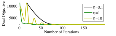
Figure 3: Progress in the dual objective for different values of $\eta$ (the factor graph is a binarized $20\times 20$ Potts grid with $8$ states; see Section 5.4 for details). For $\eta=0.1$, progress is too slow; for $\eta=10$ there are strong oscillations, which makes the algorithm slow to take off. In this example, convergence is faster with an intermediate value, $\eta=1$.

4.4.2 Primal and dual residuals

Recall from Proposition 3 that the projected subgradient algorithm yields optimality certificates, if the relaxation is tight (i.e., if the solution of the LP-MAP problem is the exact MAP), whereas in problems with a relaxation gap, it is harder to decide when to stop. It would be desirable to have similar guarantees concerning the relaxed primal. A general weakness of subgradient algorithms is that they do not have this capacity, being usually stopped rather arbitrarily after a given number of iterations. In contrast, ADMM allows keeping track of primal and dual residuals (Boyd et al., 2011), based on which it is possible to obtain certificates, not only for the primal solution (if the relaxation is tight), but also to terminate when a near optimal relaxed primal solution has been found. The primal residual $r_{P}^{(t)}$ is the amount by which the agreement constraints are violated,

$$r_{P}^{(t)}=\frac{\sum_{(i,\alpha)\in\mathcal{E}}\|\mathbf{M}_{i\alpha}\boldsymbol{q}_{\alpha}^{(t)}-\boldsymbol{p}_{i}^{(t)}\|^{2}}{\sum_{(i,\alpha)\in\mathcal{E}}|{\mathcal{Y}}_{i}|}\in[0,1],$$ (36)

where the constant in the denominator ensures that $r_{P}^{(t)}\in[0,1]$. The dual residual $r_{D}^{(t)}$,

$$r_{D}^{(t)}=\frac{\sum_{(i,\alpha)\in\mathcal{E}}\|\boldsymbol{p}_{i}^{(t)}-\boldsymbol{p}_{i}^{(t-1)}\|^{2}}{\sum_{(i,\alpha)\in\mathcal{E}}|{\mathcal{Y}}_{i}|}\in[0,1],$$ (37)

is the amount by which a dual optimality condition is violated (Boyd et al., 2011). We adopt as stopping criterion that these two residuals fall below a threshold, e.g., $10^{-6}$.

4.4.3 Approximate solutions of the local subproblems

The next proposition states that convergence may still hold, even if the local subproblems are solved approximately, provided the sequence of errors is summable. The importance of this result will be clear in Section 6, where we describe a general iterative algorithm for solving the local quadratic subproblems. Essentially, Proposition 6 allows these subproblems to be solved numerically up to some accuracy without compromising global convergence, as long as the accuracy of the solutions improves sufficiently fast over ADMM iterations.

Proposition 6 (Eckstein and Bertsekas, 1992)

Let $\eta_{t}=\eta$, $\widehat{\boldsymbol{q}}$ contain the exact solutions of (31), and $\tilde{\boldsymbol{q}}$ those produced by an approximate algorithm. Then Proposition 5 still holds, provided that

$$\sum_{t=1}^{\infty}\|\widehat{\boldsymbol{q}}-\tilde{\boldsymbol{q}}\|<\infty.$$ (38)

4.4.4 Convergence rate

Although ADMM was invented in the 1970s, its convergence rate was unknown until recently. The next proposition states the $O(1/\epsilon)$ iteration bound of AD³, asymptotically equivalent to that of the algorithm of Jojic et al. (2010), therefore better than the $O(1/\epsilon^{2})$ bound of Algorithm 1.

Proposition 7

Assume the conditions of Proposition 5. Let $\boldsymbol{\lambda}^{*}$ be a solution of the dual problem (18), $\bar{\boldsymbol{\lambda}}_{T}:=\sum_{t=1}^{T}\boldsymbol{\lambda}^{(t)}$ be the “averaged” Lagrange multipliers after $T$ iterations of AD³, and $g(\bar{\boldsymbol{\lambda}}_{T})$ the corresponding estimate of the dual objective. Then, $g(\bar{\boldsymbol{\lambda}}_{T})-g(\boldsymbol{\lambda}^{*})\leq\epsilon$ after $T\leq O(C/\epsilon)$ iterations, where $C$ satisfies

$$C\leq\frac{5\eta}{2}\sum_{i\in\mathcal{V}}|\mathcal{N}(i)|\times(1-|{\mathcal{Y}}_{i}|^{-1})+\frac{5}{2\eta}\|\boldsymbol{\lambda}^{*}\|^{2}.$$ (39)

Proof: The proof (detailed in Appendix A) uses recent results of He and Yuan (2011) and Wang and Banerjee (2012), concerning convergence of ADMM in a variational inequality setting.   

As expected, the bound (39) increases with the number of overlapping variables, the size of the sets ${\mathcal{Y}}_{i}$, and the magnitude of the optimal dual vector $\boldsymbol{\lambda}^{*}$. Note that if there is a good estimate of $\|\boldsymbol{\lambda}^{*}\|$, then (39) can be used to choose a step size $\eta$ that minimizes the bound. Moreover, unlike the $O(1/\epsilon)$ bound of the accelerated method of Jojic et al. (2010), which requires specifying $\epsilon$ beforehand, AD³ does not require pre-specifying a desired accuracy.

The bounds derived so far for all these algorithms are with respect to the dual problem—an open problem is to obtain bounds related to primal convergence.

4.4.5 Runtime and caching strategies

In practice, considerable speed-ups can be achieved by caching the subproblems, a strategy which has also been proposed for the projected subgradient algorithm (Koo et al., 2010). After a few iterations, many variables $\boldsymbol{p}_{i}$ reach a consensus (i.e., $\boldsymbol{p}_{i}^{(t)}=\boldsymbol{q}_{i\alpha}^{(t+1)},\forall\alpha\in\mathcal{N}(i)$) and enter an idle state: they are left unchanged by the $\boldsymbol{p}$-update (34), and so do the Lagrange variables $\boldsymbol{\lambda}^{(t+1)}_{i\alpha}$ (30)). If at iteration $t$ all variables in a subproblem at factor $\alpha$ are idle, then $\boldsymbol{q}_{\alpha}^{(t+1)}=\boldsymbol{q}_{\alpha}^{(t)}$, hence the corresponding subproblem does not need to be solved. Typically, many variables and subproblems enter this idle state after the first few rounds. We will show the practical benefits of caching in the experimental section (Section 7.5).

4.5 Exact Inference with Branch-and-Bound

Recall that AD³, as just described, solves the LP-MAP relaxation of the actual problem. In some problems, this relaxation is tight (in which case a certificate of optimality will be obtained), but this is not always the case. When a fractional solution is obtained, it is desirable to have a strategy to recover the exact MAP solution.

Two observations are noteworthy. First, as we saw in Section 2.3, the optimal value of the relaxed problem LP-MAP provides an upper bound to the original problem MAP. In particular, any feasible dual point provides an upper bound to the original problem’s optimal value. Second, during execution of the AD³ algorithm, we always keep track of a sequence of feasible dual points (as guaranteed by Proposition 5, item 4). Therefore, each iteration constructs tighter and tighter upper bounds. In recent work (Das2012StarSEM), we proposed a branch-and-bound search procedure that finds the exact solution of the ILP. The procedure works recursively as follows:

1. Initialize $L=-\infty$ (our best value so far).

2. Run Algorithm 2. If the solution $\boldsymbol{p}^{*}$ is integer, return $\boldsymbol{p}^{*}$ and set $L$ to the objective value. If along the execution we obtain an upper bound less than $L$, then Algorithm 2 can be safely stopped and return “infeasible”—this is the bound part. Otherwise (if $\boldsymbol{p}^{*}$ is fractional) go to step 3.

3. Find the “most fractional” component of $\boldsymbol{p}^{*}$ (call it $p_{j}^{*}(.))$ and branch: for every $y_{j}\in{\mathcal{Y}}_{j}$, constrain $p_{j}(y_{j})=1$ and go to step 2, eventually obtaining an integer solution $\boldsymbol{p}^{*}|_{y_{j}}$ or infeasibility. Return the $\boldsymbol{p}^{*}\in\{\boldsymbol{p}^{*}|_{y_{j}}\}_{y_{j}\in{\mathcal{Y}}_{j}}$ that yields the largest objective value.

Although this procedure has worst-case exponential runtime, in many problems for which the relaxations are near-exact it is found empirically very effective. We will see one example in Section 7.4.

5 Local Subproblems in AD³

5.1 Introduction

This section shows how to solve the AD³ local subproblems (31) exactly and efficiently, in several cases, including Ising models and logic constraint factors. These results will be complemented in Section 6, where a new procedure to handle arbitrary factors widens the applicability of AD³.

By subtracting a constant from the objective (31), re-scaling, and turning the maximization into a minimization, the problem can be written more compactly as

$$\mathrm{minimize}\quad \displaystyle\frac{1}{2}\sum_{i\in\mathcal{N}(\alpha)}\|\boldsymbol{q}_{i\alpha}-\boldsymbol{a}_{i}\|^{2}-{\boldsymbol{b}_{\alpha}}^{\top}{\boldsymbol{q}_{\alpha}}$$

with respect to $$\boldsymbol{q}_{\alpha}\in\Delta^{|{\mathcal{Y}}_{\alpha}|},\,\,\boldsymbol{q}_{i\alpha}\in\mathbb{R}^{|{\mathcal{Y}}_{i}|},\,\,\forall i\in\mathcal{N}(\alpha)$$

subject to $$\boldsymbol{q}_{i\alpha}=\mathbf{M}_{i\alpha}\boldsymbol{q}_{\alpha},\,\,\forall i\in\mathcal{N}(\alpha).$$ (40)

where $\boldsymbol{a}_{i}:=\boldsymbol{p}_{i}+\eta^{-1}(\boldsymbol{\theta}_{i\alpha}+\boldsymbol{\lambda}_{i\alpha})$ and $\boldsymbol{b}_{\alpha}=\eta^{-1}\boldsymbol{\theta}_{\alpha}$.

We show that (5.1) has a closed-form solution or can be solved exactly and efficiently, in several cases; e.g., for Ising models, for factor graphs imposing first-order logic (FOL) constraints, and for Potts models (after binarization). In these cases, AD³ and the projected subgradient algorithm have (asymptotically) the same computational cost per iteration, up to a logarithmic factor.

5.2 Ising Models

Ising models are factor graphs containing only binary pairwise factors. A binary pairwise factor (say, $\alpha$) is one connecting two binary variables (say, $Y_{1}$ and $Y_{2}$); thus ${\mathcal{Y}}_{1}={\mathcal{Y}}_{2}=\{0,1\}$ and ${\mathcal{Y}}_{\alpha}=\{00,01,10,11\}$. Given that $\boldsymbol{q}_{1\alpha},\boldsymbol{q}_{2\alpha}\in\Delta^{2}$, we can write $\boldsymbol{q}_{1\alpha}=(1-z_{1},z_{1})$, $\boldsymbol{q}_{2\alpha}=(1-z_{2},z_{2})$. Furthermore, since $\boldsymbol{q}_{\alpha}\in\Delta^{4}$ and marginalization requires that $q_{\alpha}(1,1)+q_{\alpha}(1,0)=z_{1}$ and $q_{\alpha}(0,1)+q_{\alpha}(1,1)=z_{2}$, we can also write $\boldsymbol{q}_{\alpha}=(1-z_{1}-z_{2}+z_{12},z_{1}-z_{12},z_{2}-z_{12},z_{12})$. Using this parametrization, problem (5.1) reduces to:

$$\mathrm{minimize}\quad \frac{1}{2}(z_{1}-c_{1})^{2}+\frac{1}{2}(z_{2}-c_{2})^{2}-c_{12}z_{12}$$

with respect to $$z_{1},z_{2},z_{12}\in[0,1]^{3}$$

subject to $$z_{12}\leq z_{1},\quad z_{12}\leq z_{2},\quad z_{12}\geq z_{1}+z_{2}-1,$$ (41)

where

$$c_{1} = \frac{a_{1\alpha}(1)+1-a_{1\alpha}(0)-b_{\alpha}(0,0)+b_{\alpha}(1,0)}{2}$$ (42)

$$c_{2} = \frac{a_{2\alpha}(1)+1-a_{2\alpha}(0)-b_{\alpha}(0,0)+b_{\alpha}(0,1)}{2}$$ (43)

$$c_{12} = \frac{b_{\alpha}(0,0)-b_{\alpha}(1,0)-b_{\alpha}(0,1)+b_{\alpha}(1,1)}{2}.$$ (44)

The next proposition (proved in Appendix B.1) establishes a closed form solution for this problem, which immediately translates into a procedure for SolveQP for binary pairwise factors.

Proposition 8

Let $[x]_{\mathbb{U}}:=\min\{\max\{x,0\},1\}$ denote projection (clipping) onto the unit interval $\mathbb{U}:=[0,1]$. The solution $(z_{1}^{*},z_{2}^{*},z_{12}^{*})$ of problem (5.2) is the following.

If $c_{12}\geq 0$,

$$(z_{1}^{*},z_{2}^{*}) = \left\{\begin{array}[]{lll}([c_{1}]_{\mathbb{U}},&[c_{2}+c_{12}]_{\mathbb{U}}),&\text{if $c_{1}>c_{2}+c_{12}$}\\ ([c_{1}+c_{12}]_{\mathbb{U}},&[c_{2}]_{\mathbb{U}}),&\text{if $c_{2}>c_{1}+c_{12}$}\\ ([(c_{1}+c_{2}+c_{12})/2]_{\mathbb{U}},&[(c_{1}+c_{2}+c_{12})/2]_{\mathbb{U}}),&\text{otherwise,}\end{array}\right.$$ (48)

$$z_{12}^{*} = \min\{z_{1}^{*},z_{2}^{*}\};$$ (49)

otherwise ,

$$(z_{1}^{*},z_{2}^{*}) = \left\{\begin{array}[]{lll}([c_{1}+c_{12}]_{\mathbb{U}},&[c_{2}+c_{12}]_{\mathbb{U}}),&\text{if $c_{1}+c_{2}+2c_{12}>1$}\\ ([c_{1}]_{\mathbb{U}},&[c_{2}]_{\mathbb{U}}),&\text{if $c_{1}+c_{2}<1$}\\ ([(c_{1}+1-c_{2})/2]_{\mathbb{U}},&[(c_{2}+1-c_{1})/2]_{\mathbb{U}}),&\text{otherwise,}\end{array}\right.$$ (53)

$$z_{12}^{*} = \max\{0,z_{1}^{*}+z_{2}^{*}-1\}.$$ (54)

5.3 Factor Graphs with First-Order Logic Constraints

Hard constraint factors allow specifying “forbidden” configurations, and have been used in error-correcting decoders (Richardson and Urbanke, 2008), bipartite graph matching (Duchi et al., 2007), computer vision (Nowozin and Lampert, 2009), and natural language processing (Sutton, 2004; Smith and Eisner, 2008). In many applications, declarative constraints are useful for injecting domain knowledge, and first-order logic (FOL) provides a natural language to express such constraints. This is particularly useful in learning from scarce annotated data (Roth and Yih, 2004; Punyakanok et al., 2005; Richardson and Domingos, 2006; Chang et al., 2008; Poon and Domingos, 2009).

In this section, we consider hard constraint factors linked to binary variables, with log-potential functions of the form

$${\theta}_{\alpha}(\boldsymbol{y}_{\alpha})=\left\{\begin{array}[]{ll}0,&\text{if $\boldsymbol{y}_{\alpha}\in\mathcal{S}_{\alpha}$}\\ -\infty,&\text{otherwise,}\end{array}\right.$$ (55)

where $\mathcal{S}_{\alpha}\subseteq\{0,1\}^{|\mathcal{N}(\alpha)|}$ is an acceptance set. These factors can be used for imposing FOL constraints, as we describe next. We define the marginal polytope $\mathcal{Z}_{\alpha}$ of a hard constraint factor $\alpha$ as the convex hull of its acceptance set,

$$\mathcal{Z}_{\alpha}=\operatorname{conv}\mathcal{S}_{\alpha}.$$ (56)

As shown in Appendix B.2, the AD³ subproblem (5.1) associated with a hard constraint factor is equivalent to that of computing an Euclidean projection onto its marginal polytope:

$$\mathrm{minimize}\quad \|\boldsymbol{z}-\boldsymbol{z}_{0}\|^{2}$$

with respect to $$\boldsymbol{z}\in\mathcal{Z}_{\alpha},$$ (57)

where $z_{0i}:=(a_{i}(1)+1-a_{i}(0))/2$, for $i\in\mathcal{N}(\alpha)$. We now show how to compute this projection for several hard constraint factors that are building blocks for writing FOL constraints. Each of these factors performs a logical function, and hence we represent them graphically as logic gates (Fig. 4).

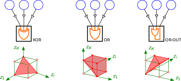
Figure 4: Logic factors and their marginal polytopes; the AD³ subproblems (5.3) are projections onto these polytopes. Left: the one-hot XOR factor (its marginal polytope is the probability simplex). Middle: the OR factor. Right: the OR-with-output factor.

One-hot XOR (Uniqueness Quantification).

The “one-hot XOR” factor linked to $K\geq 1$ binary variables is defined through the following potential function:

$${\theta}_{\mathrm{XOR}}(y_{1},\ldots,y_{K}):=\left\{\begin{array}[]{ll}0&\text{if $\exists!k\in\{1,\ldots,K\}$ s.t. $y_{k}=1$}\\ -\infty&\text{otherwise,}\end{array}\right.$$ (58)

where $\exists!$ denotes “there is one and only one.” The name “one-hot XOR” stems from the following fact: for $K=2$, $\exp({\theta}_{\mathrm{XOR}}(.))$ is the logic eXclusive-OR function; the prefix “one-hot” expresses that this generalization to $K>2$ only accepts configurations with precisely one “active” input (not to be mistaken with other XOR generalizations commonly used for parity checks). The XOR factor can be used for binarizing a categorical variable, and to express a statement in FOL of the form $\exists!x:R(x)$.

From (56), the marginal polytope associated with the one-hot XOR factor is

$$\mathcal{Z}_{\mathrm{XOR}}=\operatorname{conv}\left\{\boldsymbol{y}\in\{0,1\}^{K}\,\,|\,\,\text{$\exists!k\in\{1,\ldots,K\}$ s.t. $y_{k}=1$}\right\}=\Delta^{K}$$ (59)

as illustrated in Fig. 4. Therefore, the AD$3$ subproblem for the XOR factor consists in projecting onto the probability simplex, a problem well studied in the literature (Brucker, 1984; Michelot, 1986; Duchi et al., 2008). In Appendix B.3, we describe a simple $O(K\log K)$ algorithm. Note that there are $O(K)$ algorithms for this problem which are slightly more involved.

OR (Existential Quantification).

This factor represents a disjunction of $K\geq 1$ binary variables,

$${\theta}_{\mathrm{OR}}(y_{1},\ldots,y_{K}):=\left\{\begin{array}[]{ll}0&\text{if $\exists k\in\{1,\ldots,K\}$ s.t. $y_{k}=1$}\\ -\infty&\text{otherwise,}\end{array}\right.$$ (60)

The OR factor can be used to represent a statement in FOL of the form $\exists x:R(x)$.

From Proposition 14, the marginal polytope associated with the OR factor is:

$$\mathcal{Z}_{\mathrm{OR}} = \operatorname{conv}\left\{\boldsymbol{y}\in\{0,1\}^{K}\,\,|\,\,\text{$\exists k\in\{1,\ldots,K\}$ s.t. $y_{k}=1$}\right\}$$ (61)

$$= \left\{\boldsymbol{z}\in[0,1]^{K}\,\,\bigg{|}\,\,\sum_{k=1}^{K}z_{k}\geq 1\right\};$$ (62)

geometrically, it is a “truncated” hypercube, as depicted in Fig. 4. We derive a $O(K\log K)$ algorithm for projecting onto $\mathcal{Z}_{\mathrm{OR}}$, using a sifting technique and a sort operation (see Appendix B.4).

Logical Variable Assignments: OR-with-output.

The two factors above define a constraint on a group of existing variables. Alternatively, we may want to define a new variable (say, $y_{K+1}$) which is the result of an operation involving other variables (say, $y_{1},\ldots,y_{K}$). Among other things, this will allow dealing with “soft constraints,” i.e., constraints that can be violated but whose violation will decrease the score by some penalty. An example is the OR-with-output factor:

$${\theta}_{\mathrm{OR-out}}(y_{1},\ldots,y_{K},y_{K+1}):=\left\{\begin{array}[]{ll}1&\text{if $y_{K+1}=y_{1}\vee\cdots\vee y_{K}$}\\ 0&\text{otherwise.}\end{array}\right.$$ (63)

This factor constrains the variable $y_{K+1}$ to indicate the existence of one or more active variables among $y_{1},\ldots,y_{K}$. It can be used to express the following statement in FOL: $T(x):=\exists z:R(x,z)$.

The marginal polytope associated with the OR-with-output factor (also depicted in Fig. 4):

$$\mathcal{Z}_{\mathrm{OR-out}} = \operatorname{conv}\left\{\boldsymbol{y}\in\{0,1\}^{K+1}\,\,\bigg{|}\,\,\text{$y_{K+1}=y_{1}\vee\cdots\vee y_{K}$}\right\}$$ (64)

$$= \left\{\boldsymbol{z}\in[0,1]^{K+1}\,\,\bigg{|}\,\,\sum_{k=1}^{K}z_{k}\geq z_{K+1},\,\,z_{k}\leq z_{K+1},\forall k\in\{1,\ldots,K\}\right\}.$$ (65)

Although projecting onto $\mathcal{Z}_{\mathrm{OR-out}}$ is slightly more complicated than the previous cases, in Appendix B.5, we propose (and prove correctness of) an $O(K\log K)$ algorithm for this task.

Negations, De Morgan’s laws, and AND-with-output.

The three factors just presented can be extended to accommodate negated inputs, thus adding flexibility. Solving the corresponding AD³ subproblems can be easily done by reusing the methods that solve the original problems. For example, it is straightforward to handle negated conjunctions (NAND),

$${\theta}_{\mathrm{NAND}}(y_{1},\ldots,y_{K}) := \left\{\begin{array}[]{ll}-\infty&\text{if $y_{k}=1$, $\forall k\in\{1,\ldots,K\}$}\\ 0&\text{otherwise,}\end{array}\right.$$ (68)

$$= {\theta}_{\mathrm{OR}}(\neg y_{1},\ldots,\neg y_{K}),$$ (69)

as well as implications (IMPLY),

$${\theta}_{\mathrm{IMPLY}}(y_{1},\ldots,y_{K},y_{K+1}) := \left\{\begin{array}[]{ll}0&\text{if $\left(y_{1}\wedge\cdots\wedge y_{K}\right)\Rightarrow y_{K+1}$}\\ -\infty&\text{otherwise}\end{array}\right.$$ (72)

$$= {\theta}_{\mathrm{OR}}(\neg y_{1},\ldots,\neg y_{K},y_{K+1}).$$ (73)

In fact, from De Morgan’s laws, $\neg\left(Q_{1}(x)\wedge\cdots\wedge Q_{K}(x)\right)$ is equivalent to $\neg Q_{1}(x)\vee\cdots\vee\neg Q_{K}(x)$, and $\left(Q_{1}(x)\wedge\cdots\wedge Q_{K}(x)\right)\Rightarrow R(x)$ is equivalent to $\left(\neg Q_{1}(x)\vee\cdots\vee\neg Q_{K}(x)\right)\vee R(x)$. Another example is the AND-with-output factor,

$${\theta}_{\mathrm{AND-out}}(y_{1},\ldots,y_{K},y_{K+1}) := \left\{\begin{array}[]{ll}0&\text{if $y_{K+1}=y_{1}\wedge\cdots\wedge y_{K}$}\\ -\infty&\text{otherwise}\end{array}\right.$$ (76)

$$= {\theta}_{\mathrm{OR-out}}(\neg y_{1},\ldots,\neg y_{K},\neg y_{K+1}),$$ (77)

which can be used to impose FOL statements of the form $T(x):=\forall z:R(x,z)$.

Let $\alpha$ be a binary constraint factor with marginal polytope $\mathcal{Z}_{\alpha}$, and $\beta$ a factor obtained from $\alpha$ by negating the $k$th variable. For notational convenience, let $\mathrm{sym}_{k}:[0,1]^{K}\rightarrow[0,1]^{K}$ be defined as $(\mathrm{sym}_{k}(\boldsymbol{z}))_{k}=1-z_{k}$ and $(\mathrm{sym}_{k}(\boldsymbol{z}))_{i}=z_{i}$, for $i\neq k$. Then, the marginal polytope $\mathcal{Z}_{\beta}$ is a symmetric transformation of $\mathcal{Z}_{\alpha}$,

$$\mathcal{Z}_{\beta} = \Bigl{\{}\boldsymbol{z}\in[0,1]^{K}\,\,\big{|}\,\,\mathrm{sym}_{k}(\boldsymbol{z})\in\mathcal{Z}_{\alpha}\Bigr{\}},$$ (78)

and, if $\mathrm{proj}_{\mathcal{Z}_{\alpha}}$ denotes the projection operator onto $\mathcal{Z}_{\alpha}$,

$$\mathrm{proj}_{\mathcal{Z}_{\beta}}(\boldsymbol{z})=\mathrm{sym}_{k}\left(\mathrm{proj}_{\mathcal{Z}_{\alpha}}(\mathrm{sym}_{k}(\boldsymbol{z}))\right).$$ (79)

Naturally, $\mathrm{proj}_{\mathcal{Z}_{\beta}}$ can be computed as efficiently as $\mathrm{proj}_{\mathcal{Z}_{\alpha}}$ and, by induction, this procedure can be generalized to an arbitrary number of negated variables.

5.4 Potts Models and Graph Binarization

Although general factors lack closed-form solutions of the corresponding AD³ subproblem (5.1), it is possible to binarize the graph, i.e., to convert it into an equivalent one that only contains binary variables and XOR factors. The procedure is as follows:

• For each variable node $i\in\mathcal{V}$, define binary variables $U_{i,y_{i}}\in\{0,1\}$, for each state $y_{i}\in{\mathcal{Y}}_{i}$; link these variables to a XOR factor, imposing $\sum_{y_{i}\in{\mathcal{Y}}_{i}}p_{i}(y_{i})=1$.

• For each factor $\alpha\in\mathcal{F}$, define binary variables $U_{\alpha,\boldsymbol{y}_{\alpha}}\in\{0,1\}$ for every $\boldsymbol{y}_{\alpha}\in{\mathcal{Y}}_{\alpha}$. For each edge $(i,\alpha)\in\mathcal{E}$ and each $y_{i}\in{\mathcal{Y}}_{i}$, link variables $\{U_{\alpha,\boldsymbol{y}_{\alpha}}\,\,|\,\,\boldsymbol{y}_{\alpha}\sim y_{i}\}$ and $\neg U_{i,y_{i}}$ to a XOR factor; this imposes the constraint $p_{i}(y_{i})=\sum_{\boldsymbol{y}_{\alpha}\sim y_{i}}q_{\alpha}(\boldsymbol{y}_{\alpha})$.

The resulting binary graph is one for which we already presented the machinery needed for solving efficiently the corresponding AD³ subproblems. As an example, for Potts models (graphs with only pairwise factors and variables that have more than two states), the computational cost per AD³ iteration on the binarized graph is asymptotically the same as that of the projected subgradient method and other message-passing algorithms; for details, see Martins2012PhDThesis.

6 An Active Set Method For Solving the AD³ Subproblems

When dealing with arbitrary factors, an alternative to binarization is to use an inexact algorithm that becomes increasingly accurate as AD³ proceeds (see Proposition 6); this increasing accuracy can be achieved by warm-starting subproblem solvers with the solutions obtained in the previous iteration. We next describe such an approach, which, remarkably, only requires a black-box solving the local MAP subproblems (functions ComputeMAP in Algorithm 1). This makes AD³ applicable to a wide range of problems, by invoking specialized combinatorial algorithms for computing the MAP for factors that impose structural constraints.

The key to our approach is the conversion of the original quadratic program (5.1) into a sequence of linear problems, accomplished via an active set method (Nocedal and Wright, 1999, Section 16.4). Let us start by writing the local subproblem in (5.1) in the compact form

minimize $$\frac{1}{2}\|\boldsymbol{u}-\boldsymbol{a}\|^{2}-\boldsymbol{b}^{\top}\boldsymbol{v}$$ (80)

with respect to $$\boldsymbol{u}\in\mathbb{R}^{\sum_{i\in\mathcal{N}(\alpha)}|{\mathcal{Y}}_{i}|},\quad\boldsymbol{v}\in\mathbb{R}^{|{\mathcal{Y}}_{\alpha}|}$$

subject to $$\boldsymbol{u}=\mathbf{M}\boldsymbol{v},\quad\mathbf{1}^{\top}\boldsymbol{v}=1,\quad\boldsymbol{v}\geq 0,$$

where $\boldsymbol{u}:=(\boldsymbol{q}_{i\alpha})_{i\in\mathcal{N}(\alpha)}$ collects all the variable marginals and $\boldsymbol{v}:=\boldsymbol{q}_{\alpha}$ is the factor marginal, and similarly for $\boldsymbol{a}:=(\boldsymbol{a}_{i})_{i\in\mathcal{N}(\alpha)}$ and $\boldsymbol{b}:=\boldsymbol{b}_{\alpha}$; finally, $\mathbf{M}:=(\mathbf{M}_{i\alpha})_{i\in\mathcal{N}(\alpha)}$, denotes a matrix with $\sum_{i}|{\mathcal{Y}}_{i}|$ rows and $|{\mathcal{Y}}_{\alpha}|$ columns. The next crucial proposition (proved in Appendix C) states that problem (80) always admits a sparse solution.

Proposition 9

Problem (80) admits a solution $\boldsymbol{v}^{*}\in\mathbb{R}^{|{\mathcal{Y}}_{\alpha}|}$ with at most $\sum_{i\in\mathcal{N}(\alpha)}|{\mathcal{Y}}_{i}|-\mathcal{N}(\alpha)+1$ non-zero components.

The fact that the solution lies in a low dimensional subspace, makes active set methods appealing, since they only keep track of an active set of variables, that is, the non-zero components. Proposition 9 shows that such an algorithm only needs to maintain at most $O(\sum_{i}|{\mathcal{Y}}_{i}|)$ elements in the active set—note the additive, rather than multiplicative, dependency on the number of values of the variables. This alleviates eventual concerns about memory and storage.

Lagrangian and Dual Problem.

Problem (80) has $O({\mathcal{Y}}_{\alpha})$ variables and constraints, a number that grows exponentially with $|\mathcal{N}(\alpha)|$. We next derive a dual formulation with only $O(\sum_{i}|{\mathcal{Y}}_{i}|)$ variables. The Lagrangian of (80) is

$$L(\boldsymbol{u},\boldsymbol{v},\boldsymbol{w},\tau,\boldsymbol{\lambda})=\frac{1}{2}\|\boldsymbol{u}-\boldsymbol{a}\|^{2}-\boldsymbol{b}^{\top}\boldsymbol{v}-\boldsymbol{w}^{\top}(\mathbf{M}\boldsymbol{v}-\boldsymbol{u})-\tau(1-\mathbf{1}^{\top}\boldsymbol{v})-\boldsymbol{\lambda}^{\top}\boldsymbol{v}.$$ (81)

Equating $\nabla_{\boldsymbol{u}}L(\boldsymbol{u},\boldsymbol{v},\boldsymbol{w},\tau,\boldsymbol{\lambda})$ and $\nabla_{\boldsymbol{v}}L(\boldsymbol{u},\boldsymbol{v},\boldsymbol{w},\tau,\boldsymbol{\lambda})$ to zero leads to the equations:

$$\boldsymbol{u} = \boldsymbol{a}-\boldsymbol{w}$$ (82)

$$\mathbf{M}^{\top}\boldsymbol{w}+\boldsymbol{b} = \tau\mathbf{1}-\boldsymbol{\lambda}.$$ (83)

Since the Lagrange variables $\boldsymbol{\lambda}$ are constrained to be non-negative, the dual problem takes the form (after replacing the maximization with a minimization and subtracting a constant),

minimize $$\frac{1}{2}\|\boldsymbol{w}-\boldsymbol{a}\|^{2}+\tau$$ (84)

with respect to $$\boldsymbol{w}\in\mathbb{R}^{\sum_{i}|{\mathcal{Y}}_{i}|},\quad{\tau}\in\mathbb{R}$$

subject to $$\mathbf{M}^{\top}\boldsymbol{w}+\boldsymbol{b}\leq\tau\mathbf{1},$$

which can be seen as a “projection with slack” onto $\{\boldsymbol{w}\,\,|\,\,\mathbf{M}^{\top}\boldsymbol{w}+\boldsymbol{b}\leq\mathbf{0}\}$. We now apply the active set method of Nocedal and Wright (1999, Section 16.4) to this problem. Letting $\boldsymbol{m}_{r}$ denote the $r$th column of matrix $\mathbf{M}$, this method keeps track of a working set of constraints assumed to be active:

$$\mathcal{W}:=\left\{r\in\{1,\ldots,|{\mathcal{Y}}_{\alpha}|\}\,\,|\,\,\boldsymbol{m}_{r}^{\top}\boldsymbol{w}+b_{r}-\tau=0\right\};$$ (85)

by complementary slackness, at the optimum, this set contains the support of $\boldsymbol{v}^{*}$.

KKT conditions.

The KKT equations of (84) are:

$$\boldsymbol{u}-\boldsymbol{a}+\boldsymbol{w}=0 \quad(\nabla_{\boldsymbol{u}}L=0)$$ (86)

$$\mathbf{M}^{\top}\boldsymbol{w}+\boldsymbol{b}=\tau\mathbf{1}-\boldsymbol{\lambda} \quad(\nabla_{\boldsymbol{v}}L=0)$$ (87)

$$\mathbf{M}\boldsymbol{v}=\boldsymbol{u}$$ (Primal feasibility) (88)

$$\mathbf{1}^{\top}\boldsymbol{v}=1$$ (Primal feasibility) (89)

$$\boldsymbol{y}\geq\mathbf{0}$$ (Primal feasibility) (90)

$$\boldsymbol{\lambda}\geq\mathbf{0}$$ (Dual feasibility) (91)

$$\boldsymbol{\lambda}^{\top}\boldsymbol{v}=\mathbf{0} \quad\text{(Complementary slackness)}.$$ (92)

We can eliminate variables $\boldsymbol{u}$ and $\boldsymbol{w}$ and reduce the above set of equations to

$$\mathbf{M}^{\top}\mathbf{M}\boldsymbol{v}+\tau\mathbf{1} = \mathbf{M}^{\top}\boldsymbol{a}+\boldsymbol{b}+\boldsymbol{\lambda}$$ (93)

$$\mathbf{1}^{\top}\boldsymbol{v} = 1$$ (94)

$$\boldsymbol{v} \geq \mathbf{0}$$ (95)

$$\boldsymbol{\lambda} \geq \mathbf{0}$$ (96)

$$\boldsymbol{\lambda}^{\top}\boldsymbol{v} = \mathbf{0}.$$ (97)

Let $\mathcal{I}$ denote the, obviously unknown, support of $\boldsymbol{v}$. The algorithm maintains the active set $\mathcal{W}$ (85), which is a guess of $\mathcal{I}$. Let $\boldsymbol{v}_{\mathcal{I}}$ and $\boldsymbol{\lambda}_{\mathcal{I}}$ be the subvectors indexed by $\mathcal{I}$ and $\mathbf{M}_{\mathcal{I}}$ be the submatrix of $\mathbf{M}$ with column indices in $\mathcal{I}$. Equations (93)–(97) imply $\boldsymbol{\lambda}_{\mathcal{I}}=\mathbf{0}$ and the system of equations

$$\left[\begin{array}[]{cc}\mathbf{M}_{\mathcal{I}}^{\top}\mathbf{M}_{\mathcal{I}}&\mathbf{1}\\ \mathbf{1}^{\top}&0\end{array}\right]\left[\begin{array}[]{c}\boldsymbol{v}_{\mathcal{I}}\\ \tau\end{array}\right]=\left[\begin{array}[]{c}\mathbf{M}_{\mathcal{I}}^{\top}\boldsymbol{a}+\boldsymbol{b}_{\mathcal{I}}\\ 1\end{array}\right].$$ (98)

If the matrix in the left-hand side is non-singular, this system has a unique solution $(\widehat{\boldsymbol{v}}_{\mathcal{I}},\widehat{\tau})$. If $\widehat{\boldsymbol{v}}$ (given by zero-padding $\widehat{\boldsymbol{v}}_{\mathcal{I}}$) and $\widehat{\tau}$ satisfy the KKT conditions ((93)–(97)), i.e., if we have $\widehat{\boldsymbol{v}}\geq\mathbf{0}$ and

$$\mathbf{M}^{\top}\mathbf{M}\widehat{\boldsymbol{v}}+\widehat{\tau}\mathbf{1} \geq \mathbf{M}^{\top}\boldsymbol{a}+\boldsymbol{b},$$ (99)

then the set $\mathcal{I}$ is correct and $\widehat{\boldsymbol{v}}$ is a solution of (80). To use this rationale algorithmically, the following two operations need to be performed:

• Solving the KKT system (98), i.e., inverting a $|\mathcal{I}|\times|\mathcal{I}|$ matrix. Since this operation is repeated after inserting or removing an element from the active set, it can be done efficiently (namely, in time $O(|\mathcal{I}|^{2})$) by keeping track of the inverse matrix. From Proposition 9, this runtime is manageable, since the size of the active set is limited by $O(\sum_{i}|{\mathcal{Y}}_{i}|)$. Note also that adding a new configuration $\boldsymbol{y}_{\alpha}$ to the active set, corresponds to inserting a new column in $\mathbf{M}_{\mathcal{I}}$ thus the matrix inversion requires updating $\mathbf{M}_{\mathcal{I}}^{\top}\mathbf{M}_{\mathcal{I}}$. From the definition of $\mathbf{M}$ and simple algebra, the $(\boldsymbol{y}_{\alpha},\boldsymbol{y}^{\prime}_{\alpha})$ entry in $\mathbf{M}^{\top}\mathbf{M}$ is simply the number of common values between the configurations $\boldsymbol{y}_{\alpha}$ and $\boldsymbol{y}^{\prime}_{\alpha}$. Hence, when a new configuration $\boldsymbol{y}_{\alpha}$ is added to the active set $\mathcal{W}$, that configuration needs to be compared with all the others already in $\mathcal{W}$.

• Checking if the constraints (99) are satisfied; by setting $\widehat{\boldsymbol{u}}=\mathbf{M}\widehat{\boldsymbol{v}}$ and $\widehat{\boldsymbol{w}}=\boldsymbol{a}-\widehat{\boldsymbol{u}}$, the constraints can be written as $\mathbf{M}^{\top}\widehat{\boldsymbol{w}}+\boldsymbol{b}\leq\widehat{\tau}\mathbf{1}$, and they hold if and only if $\max_{r\in{\mathcal{Y}}_{\alpha}}\boldsymbol{m}_{r}^{\top}\widehat{\boldsymbol{w}}+\boldsymbol{b}_{r}\leq\widehat{\tau}.$ Hence, checking the constraints only involves computing this maximum, which, interestingly, coincides with finding the MAP configuration of factor $\alpha$ with variable log-potentials $\widehat{\boldsymbol{w}}$ and factor log-potentials $\boldsymbol{b}$. This can be obtained through the function ComputeMAP.

Active set algorithm.

Algorithm 3 formally describes the complete procedure. At each iteration $s$, an active set $\mathcal{W}_{s}$ stores the current guess of the support of $\boldsymbol{v}$. The active set is initialized arbitrarily: e.g., in the first outer iteration of AD³, it is initialized with the single output $\boldsymbol{y}_{\alpha}$, which is the MAP configuration corresponding to log-potentials $\boldsymbol{a}$ and $\boldsymbol{b}$; in subsequent AD³ iterations, it is warm-started with the solution obtained in the previous iteration. At each inner iteration, the KKT system (98) is solved given the current active set.

If the solution is the same as in the previous round, a black-box ComputeMAP is invoked to check for KKT violations; if there are none, the algorithm returns; otherwise, it adds the most violated constraint to the active set. If the solution of the KKT system $\widehat{\boldsymbol{v}}$ is different from the previous one ($\widehat{\boldsymbol{v}}_{s}$), the algorithm sets $\boldsymbol{v}_{s+1}:=(1-\alpha_{s})\boldsymbol{v}_{s}+\alpha_{s}\widehat{\boldsymbol{v}}$, where the step size $\alpha_{s}$ is chosen by line search to yield the largest improvement in the objective, while keeping the constraints satisfied; this has a closed form solution (Nocedal and Wright, 1999, p. 457).

Algorithm 3 Active Set Algorithm for Solving a General AD³ Subproblem

1:  input: Parameters $\boldsymbol{a},\boldsymbol{b},\mathbf{M}$, starting point $\boldsymbol{v}_{0}$

2:  initialize $\mathcal{W}_{0}$ as the support of $\boldsymbol{v}_{0}$

3:  for $s=0,1,2,\ldots$ do

4:     solve the KKT system and obtain $\widehat{\boldsymbol{v}}$ and $\widehat{\tau}$ (Eq. 98)

5:     if $\widehat{\boldsymbol{v}}=\boldsymbol{v}_{s}$ then

6:        compute $\widehat{\boldsymbol{u}}:=\mathbf{M}\widehat{\boldsymbol{v}}$ and $\widehat{\boldsymbol{w}}:=\boldsymbol{a}-\widehat{\boldsymbol{u}}$

7:        obtain the tighter constraint $r$ via $\boldsymbol{e}_{r}=\text{{\sc ComputeMAP}}({\boldsymbol{b}}+\mathbf{M}^{\top}\widehat{\boldsymbol{w}})$

8:        if $\boldsymbol{m}_{r}^{\top}\widehat{\boldsymbol{w}}+\boldsymbol{b}_{r}\leq\widehat{\tau}$ then

9:           return solution $\widehat{\boldsymbol{u}}$ and $\widehat{\boldsymbol{v}}$

10:        else

11:           add the most violated constraint to the active set: $\mathcal{W}_{s+1}:=\mathcal{W}_{s}\cup\{r\}$

12:        end if

13:     else

14:        compute the interpolation constant $\alpha_{s}:=\min\left\{1,\min_{r\in\mathcal{W}_{s}\,\,\text{s.t.}\,\,v_{s,r}>\widehat{v}_{r}}\frac{v_{s,r}}{v_{s,r}-\widehat{v}_{r}}\right\}$

15:        set $\boldsymbol{v}_{s+1}:=(1-\alpha_{s})\boldsymbol{v}_{s}+\alpha_{s}\widehat{\boldsymbol{v}}$

16:        if there are blocking constraints then

17:           pick a blocking constraint $r$

18:           remove that blocking constraint from the active set: $\mathcal{W}_{s+1}:=\mathcal{W}_{s}\setminus\{r\}$

19:        end if

20:     end if

21:  end for

22:  output: $\widehat{\boldsymbol{u}}$ and $\widehat{\boldsymbol{v}}$

Each iteration of Algorithm 3 always improves the dual objective and, with a suitable strategy to prevent cycles and stalling, the algorithm is guaranteed to stop after a finite number of steps (Nocedal and Wright, 1999, Theorem 16.5). In practice, since it is run as a subroutine of AD³, Algorithm 3 does not need to be run to optimality, which is particularly convenient in early iterations of AD³ (this is supported by Proposition 6). The ability to warm-start each outer AD³ iteration with the solution from the previous round is very useful in practice: we have observed that, thanks to this warm-starting strategy, very few inner iterations are typically necessary for the correct active set to be identified. We will provide some empirical evidence in Section 7.5.

7 Experiments

7.1 Baselines and Problems

In this section, we provide an empirical comparison between AD³ (Algorithm 2) and four other algorithms: Star-MSD (Sontag et al., 2011), which is an accelerated version of the max-sum diffusion algorithm (Kovalevsky and Koval, 1975; Werner, 2007); generalized MPLP (Globerson and Jaakkola, 2008); the projected subgradient algorithm of Komodakis et al. (2007) (Algorithm 1) and its accelerated version introduced by Jojic et al. (2010) (mentioned in Subsection 4.1). All these algorithms address the LP-MAP problem; the first are message-passing methods performing block coordinate descent in the dual, whereas the last two are based on dual decomposition. All the baselines have the same algorithmic complexity per iteration, which is asymptotically the same as that of the AD³ applied to a binarized graph, but different from that of AD³ with the active set method.

We compare the performance of the algorithms above in several datasets, including synthetic Ising and Potts models, protein design problems, and two problems in natural language processing: frame-semantic parsing and non-projective dependency parsing. The graphical models associated with these problems are quite diverse, containing pairwise binary factors (AD³ subproblems solved as described in Section 5.2), first-order logic factors (addressed using the tools of Section 5.3), dense factors, and structured factors (tackled with the active set method of Section 6).

7.2 Synthetic Ising and Potts Models

Ising models.

Fig. 5 reports experiments with random Ising models, with single-node log-potentials chosen as ${\theta}_{i}(1)-{\theta}_{i}(0)\sim\mathcal{U}[-1,1]$ and random edge couplings in $\mathcal{U}[-\rho,\rho]$, where $\rho\in\{0.5,1,1.5,2\}$. Decompositions are edge-based for all methods. For MPLP and Star-MSD, primal feasible solutions $(\widehat{y}_{i})_{i\in\mathcal{V}}$ are obtained by decoding the single node messages (Globerson and Jaakkola, 2008); for the dual decomposition methods, $\widehat{y}_{i}=\operatorname*{argmax}_{y_{i}}p_{i}(y_{i})$.

We observe that the projected subgradient is the slowest, taking a long time to find a “good” primal feasible solution, arguably due to the large number of components. The accelerated dual decomposition method (Jojic et al., 2010) is also not competitive in this setting, as it takes many iterations to reach a near-optimal region. MPLP performs slightly better than Star-MSD and both are comparable to AD³ in terms of convergence of the dual objective. However, AD³ outperforms all competitors at obtaining a “good” feasible primal solution in early iterations (it retrieved the exact MAP in all cases, in no more than $200$ iterations). We conjecture that this rapid progress in the primal is due to the penalty term in the augmented Lagrangian (Eq. 27), which pushes for a feasible primal solution of the relaxed LP.

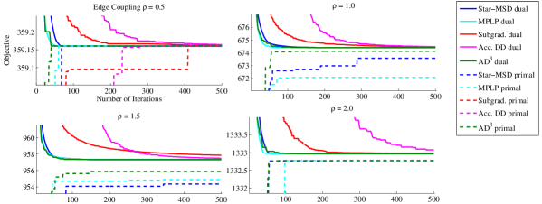
Figure 5: Evolution of the dual objective and the best primal feasible one in the experiments with $30\times 30$ random Ising models, generated as described in the main text. For the subgradient method, the step sizes are $\eta_{t}\!=\!\eta_{0}/t$, with $\eta_{0}$ adjusted (with halving steps) to yield the maximum dual improvement in $10$ iterations (those steps are not plotted). For accelerated dual decomposition, the most favorable $\epsilon\!\in\!\{0.1,1,10,100\}$ is chosen. AD³ uses $\eta\!=\!5.0$.

Potts models.

The effectiveness of AD³ in the non-binary case is assessed using random Potts models, with single-node log-potentials chosen as ${\theta}_{i}(y_{i})\sim\mathcal{U}[-1,1]$ and pair-wise log-potentials as ${\theta}_{ij}(y_{i},y_{j})\sim\mathcal{U}[-10,10]$ if $y_{i}=y_{j}$ and $0$ otherwise. The two baselines (MPLP and accelerated dual decomposition) use the same edge decomposition as before, since they handle multi-valued variables; for AD³, the graph is binarized (see Section 5.4). As observed in the left plot of Fig. 6, MPLP decreases the objective very rapidly in the beginning and then slows down; the accelerated dual decomposition algorithm, although slower in early iterations, converging faster. AD³ converges as fast as the accelerated dual decomposition algorithm, and is almost as fast as MPLP in early iterations. The right plot of Fig. 6 shows that AD³ with the subproblems solved by the active set method (see Section 6) clearly outperforms the binarization-based version. Notice that since AD³ with the active set method involves more computation per iteration, we plot the objective values with respect to runtime.

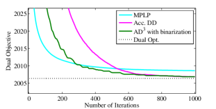
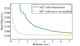
Figure 6: Evolution of the dual objective in the experiments with random $20\times 20$ Potts models with $8$-valued nodes, generated as described in the main text. For the accelerated dual decomposition algorithm, $\epsilon=1.0$. For AD³, the left plot used $\eta=0.5$ and the right one $\eta=1$ (found to be the most favorable choice in $\{0.01,0.1,1,10\}$). In the active set method, the maximum number of inner iterations is $10$.

7.3 Protein Design

We compare AD³ with the MPLP implementation of Sontag et al. (2008) in the benchmark protein design problems of Yanover et al. (2006). In these problems, the input is a three-dimensional shape, and the goal is to find the most stable sequence of amino acids in that shape. The problems can be represented as a pairwise factor graphs, whose variables correspond to the identity of amino acids and rotamer configurations, thus having hundreds of possible states. Fig. 7 plots the evolution of the dual objective over runtime, for two of the largest problem instances, i.e., those with 3167 (1fbo) and 1163 (1kw4) factors. These plots are representative of the typical performance obtained in other instances. In both cases, MPLP steeply decreases the objective at early iterations, but then reaches a plateau with no further significant improvement. AD³ rapidly surpasses MPLP in obtaining a better dual objective. Finally, observe that although earlier iterations of AD³ take longer than those of MPLP, this cost is amortized in later iterations, by warm-starting the active set method.

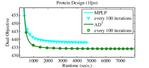
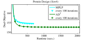
Figure 7: Protein design experiments (see main text for details). In AD³, $\eta$ is adjusted as proposed by Boyd et al. (2011), initialized at $\eta=1.0$ and the subproblems are solved by the proposed active set method, which shows better performance that the binarization-based version. Although the plots are with respect to runtime, they also indicate iteration counts.

7.4 Frame-Semantic Parsing

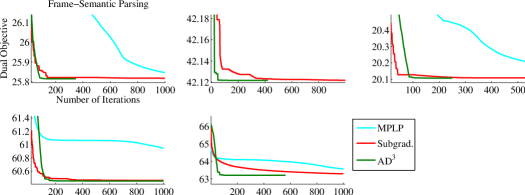
Figure 8: Experiments in five frame-semantic parsing problems (Das, 2012, Section 5.5). The projected subgradient uses $\eta_{t}=\eta_{0}/t$, with $\eta_{0}=1.0$ (found to be the best choice for all examples). In AD³, $\eta$ is adjusted as proposed by Boyd et al. (2011), initialized at $\eta=1.0$.

We now report experiments on a natural language processing task involving logic constraints: frame-semantic parsing, using the FrameNet lexicon (Fillmore, 1976). The goal is to predict the set of arguments and roles for a predicate word in a sentence, while respecting several constraints about the frames that can be evoked. The resulting graphical models are binary constrained factor graphs with FOL constraints (see Das2012StarSEM for details about this task). Fig. 8 shows the results of AD³, MPLP, and projected subgradient on the five most difficult problems (which have between $321$ and $884$ variables, and between $32$ and $59$ factors), the ones in which the LP relaxation is not tight. Unlike MPLP and projected subgradient, which did not converge after 1000 iterations, AD³ achieves convergence in a few hundreds of iterations for all but one example. Since these examples have a fractional LP-MAP solution, we applied the branch-and-bound procedure described in Section 4.5 to obtain the exact MAP for these examples. The whole dataset contains 4,462 instances, which were parsed by this exact variant of the AD³ algorithm in only $4.78$ seconds, against $43.12$ seconds of CPLEX, a state-of-the-art commercial ILP solver.

7.5 Dependency Parsing

The final set of experiments assesses the ability of AD³ to handle problems with structured factors. The task is dependency parsing (illustrated in the left part of Fig. 9), an important problem in natural language processing (Eisner, 1996; McDonald et al., 2005), to which dual decomposition has been recently applied (Koo et al., 2010). We use an English dataset derived from the Penn Treebank (PTB)(Marcus et al., 1993), converted to dependencies by applying the head rules of Yamada and Matsumoto (2003); we follow the common procedure of training in sections §02–21 (39,832 sentences), using §22 as validation data (1,700 sentences), and testing on §23 (2,416 sentences). We ran a part-of-speech tagger on the validation and test splits, and devised a linear model using various features depending on words, part-of-speech tags, and arc direction and length. Our features decompose over the parts illustrated in the right part of Fig. 9. We consider two different models in our experiments: a second order model with scores for arcs, consecutive siblings, and grandparents; a full model, which also has scores for arbitrary siblings and head bigrams.

Figure 9: Left: example of a sentence (input) and its dependency parse tree (output to be predicted); this is a directed spanning tree where each arc $(h,m)$ represent a syntactic relationships between a head word $h$ and the a modifier word $m$. Right: the parts used in our models. Arcs are the basic parts: any dependency tree can be “read out” from its arcs. Consecutive siblings and grandparent parts introduce horizontal and vertical Markovization. We break the horizontal Markovianity via all siblings parts (which look at arbitrary pairs of siblings, not necessarily consecutive). Inspired by transition-based parsers, we also adopt head bigram parts, which look at the heads attached to consecutive words.

If only scores for arcs were used, the problem of obtaining a parse tree with maximal score could be solved efficiently with a maximum directed spanning tree algorithm (Chu and Liu, 1965; Edmonds, 1967; McDonald et al., 2005); the addition of any of the other scores makes the problem NP-hard (McDonald and Satta, 2007). A factor graph representing the second order model, proposed by Smith and Eisner (2008) and Koo et al. (2010), contains binary variables representing the candidate arcs, a hard-constraint factor imposing the tree constraint, and head automata factors modeling the sequences of consecutive siblings and grandparents. The full model has additional binary pairwise factors for each possible pair of siblings (significantly increasing the number of factors), and a sequential factor modeling the sequence of heads. We have shown in previous work (Martins et al., 2011a) that MPLP and the accelerated dual decomposition methods are not competitive with AD³ for this task, hence we leave them out of this experiment.

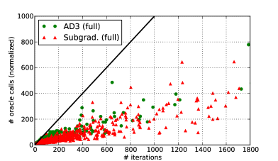
Figure 10: Number of calls to ComputeMAP for AD³ and projected subgradient, as a function of the number of iterations. The number of calls is normalized by dividing by the number of factors: in the subgradient method, this number would equal the number of iterations if there was no caching (black line); each iteration of AD³ runs $10$ iterations of the active set method, thus without caching or warm-starting the normalized number of calls would be ten times the number of AD³ iterations. Yet, it is clear that both algorithms make significantly fewer calls. Remarkably, after just a few iterations, the number of calls made by the AD³ and the subgradient algorithms are comparable, which means that the number of active set iterations is quickly amortized during the execution of AD³.

Fig. 10 illustrates the remarkable speed-ups that the caching and warm-starting procedures bring to both the AD³ and projected subgradient algorithms. A similar conclusion was obtained by Koo et al. (2010) for projected subgradient and by Martins et al. (2011b) for AD³ in a different factor graph. Fig. 11 shows average runtimes for both algorithms, as a function of the sentence length, and plots the percentage of instances for which the exact solution was obtained, along with a certificate of optimality. For the second-order model, AD³ was able to solve all the instances to optimality, and in 98.2% of the cases, the LP-MAP was exact. For the full model, AD³ solved 99.8% of the instances to optimality, being exact in 96.5% of the cases. For the second order model, we obtained in the test set (PTB §23) a parsing speed of 1200 tokens per second and an unlabeled attachment score of 92.48% (fraction of correct dependency attachments excluding punctuation). For the full model, we obtained a speed of  900 tokens per second and a score of 92.62%. All speeds were measured in a desktop PC with Intel Core i7 CPU 3.4 GHz and 8GB RAM. The parser is publicly available as an open-source project in http://www.ark.cs.cmu.edu/TurboParser.

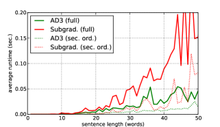
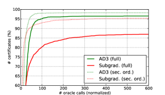
Figure 11: Left: average runtime in PTB §22, as a function of sentence length. Right: percentage of instances, as a function of the normalized number of ComputeMAP calls (see the caption of Fig. 10), for which the exact solution was obtained along with a certificate of optimality. The maximum number of iterations is 2000 for both methods.

8 Recent Related Work

During the preparation of this paper, and following our earlier work (Martins et al., 2010a, 2011a), a few related methods have appeared. Meshi and Globerson (2011) also applied ADMM to MAP inference in graphical models, although addressing the dual problem (the one underlying the MPLP algorithm) rather than the primal. Yedidia et al. (2011) proposed the divide-and-concur algorithm for LDPC (low-density parity check) decoding, which shares aspects of AD³, and can be seen as an instance of non-convex ADMM. More recently, Barman et al. (2011) proposed an algorithm analogous to AD³ for the same LDPC decoding problem; in that algorithm, the subproblems correspond to projections onto the parity polytope, for which they have derived an efficient $O(L\log L)$ algorithm, where $L$ is the number of parity check bits.

9 Conclusions

We introduced AD³, a new LP-MAP inference algorithm based on the alternating directions method of multipliers (ADMM) (Glowinski and Marroco, 1975; Gabay and Mercier, 1976).

AD³ enjoys the modularity of dual decomposition methods, but achieves faster consensus, by penalizing, for each subproblem, deviations from the current global solution.

Blending older and newer results for ADMM (Glowinski and Le Tallec, 1989; Eckstein and Bertsekas, 1992; He and Yuan, 2011; Wang and Banerjee, 2012), we showed that AD³ converges to an $\epsilon$-accurate solution with an iteration bound of $O(1/\epsilon)$.

AD³ can handle factor graphs with hard constraints in first-order logic, using efficient procedures for projecting onto the marginal polytopes of the corresponding hard constraint factors. This opens the door for using AD³ in problems with declarative constraints (Roth and Yih, 2004; Richardson and Domingos, 2006). Up to a logarithmic term, the asymptotic cost of projecting onto those polytopes is the same as that of message passing. A closed-form solution of the AD³ subproblem was also derived for pairwise binary factors.

We introduced a new active set method for solving the AD³ subproblems for arbitrary factors. This method requires only a local MAP oracle, as the projected subgradient method (see Section 3). The active set method is particulary suitable for these problems, since it can take advantage of warm starting and it deals well with sparse solutions—which are guaranteed by Proposition 9. We also show how AD³ can be wrapped in a branch-and-bound procedure to retrieve the exact MAP.

Experiments with synthetic and real-world datasets have shown that AD³ is able to solve the LP-MAP problem more efficiently than other methods for a variety of problems, including MAP inference in Ising and Potts models, protein design, frame-semantic parsing, and dependency parsing.

Our contributions open several directions for future research. One possible extension is to replace the quadratic (Euclidean) penalty of ADMM by a general Bregman divergence (notice that an entropic penalty would not lead to the same subproblems as in Jojic et al. (2010)). Although extensions of ADMM to Bregman penalties have been considered in the literature, to the best of our knowledge, convergence has only been shown for quadratic penalties. The convergence proofs, however, can be trivially extended to Mahalanobis distances, since they correspond to an affine transformation of the subspace defined by the equality constraints of Eq. 21. Simple operations, such as scaling these constraints, do not affect the algorithms that are used to solve the subproblems, thus AD³ can be generalized by including scaling parameters.

Since the AD³ subproblems can be solved in parallel, significant speed-ups may be obtained in multi-core architectures or using GPU programming. This has been shown to be very useful for large-scale message-passing inference in graphical models (Low et al., 2010).

The branch-and-bound algorithm for obtaining the exact MAP deserves further experimental study. An advantage of AD³ is its ability to quickly produce sharp upper bounds, useful for embedding in a branch-and-bound procedure. For many problems, there are effective rounding procedures that can also produce lower bounds, which can be exploited for guiding the search. There are also alternatives to branch-and-bound, such as tightening procedures (Sontag et al., 2008), which progressively add larger factors to decrease the duality gap. The variant of AD³ with the active set method can be used to handle these larger factors.

Acknowledgments.

A. M. was supported by a FCT/ICTI grant through the CMU-Portugal Program, and also by Priberam. This work was partially supported by the FET programme (EU FP7), under the SIMBAD project (contract 213250), and by a FCT grant PTDC/EEA-TEL/72572/2006. N. S. was supported by NSF CAREER IIS-1054319. E. X. was supported by AFOSR FA9550010247, ONR N000140910758, NSF CAREER DBI-0546594, NSF IIS-0713379, and an Alfred P. Sloan Fellowship.

Appendix A Proof of Convergence Rate of AD³

In this appendix, we show the $O(1/\epsilon)$ convergence bound of the ADMM algorithm. We use a recent result established by Wang and Banerjee (2012) regarding convergence in a variational setting, from which we derive the convergence of ADMM in the dual objective. We then consider the special case of AD³, interpreting the constants in the bound in terms of properties of the graphical model.

We start with the following proposition, which states the variational inequality associated with the Lagrangian saddle point problem associated with (20),

$$\min_{\boldsymbol{\lambda}\in\Lambda}\max_{\boldsymbol{q}\in\mathcal{Q},\boldsymbol{p}\in\mathcal{P}}L(\boldsymbol{q},\boldsymbol{p},\boldsymbol{\lambda}),$$ (100)

where $L(\boldsymbol{q},\boldsymbol{p},\boldsymbol{\lambda}):=f_{1}(\boldsymbol{q})+f_{2}(\boldsymbol{p})+{\boldsymbol{\lambda}}^{\top}{(\mathbf{A}\boldsymbol{q}+\mathbf{B}\boldsymbol{p}-\boldsymbol{c})}$ is the standard Lagrangian, and

$$\Lambda:=\{\boldsymbol{\lambda}\,\,|\,\,\max_{\boldsymbol{q}\in\mathcal{Q},\boldsymbol{p}\in\mathcal{P}}L(\boldsymbol{q},\boldsymbol{p},\boldsymbol{\lambda})<\infty\}.$$

Proposition 10 (Variational inequality)

Let $\mathcal{W}:=\mathcal{Q}\times\mathcal{P}\times\Lambda$. Given $\boldsymbol{w}=(\boldsymbol{q},\boldsymbol{p},\boldsymbol{\lambda})\in\mathcal{W}$, define $h(\boldsymbol{w}):=f_{1}(\boldsymbol{q})+f_{2}(\boldsymbol{p})$ and $F(\boldsymbol{w}):=(\mathbf{A}^{\top}\boldsymbol{\lambda},\mathbf{B}^{\top}\boldsymbol{\lambda},-(\mathbf{A}\boldsymbol{q}+\mathbf{B}\boldsymbol{p}-\boldsymbol{c}))$. Then, $\boldsymbol{w}^{*}:=(\boldsymbol{q}^{*},\boldsymbol{p}^{*},\boldsymbol{\lambda}^{*})\in\mathcal{W}$ is a primal-dual solution of Eq. 100 if and only if:

$$\forall\boldsymbol{w}\in\mathcal{W},\quad h(\boldsymbol{w})-h(\boldsymbol{w}^{*})+{(\boldsymbol{w}-\boldsymbol{w}^{*})}^{\top}{F(\boldsymbol{w}^{*})}\leq 0.$$ (101)

Proof: Assume $\boldsymbol{w}^{*}$ is a primal-dual solution of Eq. 100. Then, from the saddle point conditions, we have for every $\boldsymbol{w}:=(\boldsymbol{q},\boldsymbol{p},\boldsymbol{\lambda})\in\mathcal{W}$:

$$L(\boldsymbol{q},\boldsymbol{p},\boldsymbol{\lambda}^{*})\leq L(\boldsymbol{q}^{*},\boldsymbol{p}^{*},\boldsymbol{\lambda}^{*})\leq L(\boldsymbol{q}^{*},\boldsymbol{p}^{*},\boldsymbol{\lambda}).$$ (102)

Hence:

$$0 \geq L(\boldsymbol{q},\boldsymbol{p},\boldsymbol{\lambda}^{*})-L(\boldsymbol{q}^{*},\boldsymbol{p}^{*},\boldsymbol{\lambda})$$ (103)

$$= f_{1}(\boldsymbol{q})+f_{2}(\boldsymbol{p})+{\boldsymbol{\lambda}^{*}}^{\top}{(\mathbf{A}\boldsymbol{q}+\mathbf{B}\boldsymbol{p}-\boldsymbol{c})}-f_{1}(\boldsymbol{q}^{*})-f_{2}(\boldsymbol{p}^{*})-{\boldsymbol{\lambda}}^{\top}{(\mathbf{A}\boldsymbol{q}^{*}+\mathbf{B}\boldsymbol{p}^{*}-\boldsymbol{c})}$$

$$= h(\boldsymbol{w})-h(\boldsymbol{w}^{*})+{\boldsymbol{q}}^{\top}{\mathbf{A}^{\top}\boldsymbol{\lambda}^{*}}+{\boldsymbol{p}}^{\top}{\mathbf{B}^{\top}\boldsymbol{\lambda}^{*}}-{(\boldsymbol{\lambda}-\boldsymbol{\lambda}^{*})}^{\top}{(\mathbf{A}\boldsymbol{q}^{*}+\mathbf{B}\boldsymbol{p}^{*}-\boldsymbol{c})}-{\boldsymbol{\lambda}^{*}}^{\top}{(\mathbf{A}\boldsymbol{q}^{*}+\mathbf{B}\boldsymbol{p}^{*})}$$

$$= h(\boldsymbol{w})-h(\boldsymbol{w}^{*})+{(\boldsymbol{w}-\boldsymbol{w}^{*})}^{\top}{F(\boldsymbol{w}^{*})}.$$

Conversely, let $\boldsymbol{w}^{*}$ satisfy Eq. 101. Taking $\boldsymbol{w}=(\boldsymbol{q}^{*},\boldsymbol{p}^{*},\boldsymbol{\lambda})$, we obtain $L(\boldsymbol{q}^{*},\boldsymbol{p}^{*},\boldsymbol{\lambda}^{*})\leq L(\boldsymbol{q}^{*},\boldsymbol{p}^{*},\boldsymbol{\lambda})$. Taking $\boldsymbol{w}=(\boldsymbol{q},\boldsymbol{p},\boldsymbol{\lambda}^{*})$, we obtain $L(\boldsymbol{q},\boldsymbol{p},\boldsymbol{\lambda}^{*})\leq L(\boldsymbol{q}^{*},\boldsymbol{p}^{*},\boldsymbol{\lambda}^{*})$. Hence $(\boldsymbol{q}^{*},\boldsymbol{p}^{*},\boldsymbol{\lambda}^{*})$ is a saddle point, and therefore a primal-dual solution.   

The next result, due to Wang and Banerjee (2012) and related to previous work by He and Yuan (2011), concerns the convergence rate of ADMM in terms of the variational inequality stated above.

Proposition 11 (Variational convergence rate)

Assume the conditions in Proposition 5. Let $\bar{\boldsymbol{w}}_{T}=\frac{1}{T}\sum_{t=1}^{T}\boldsymbol{w}^{t}$, where $\boldsymbol{w}^{t}:=(\boldsymbol{q}^{t},\boldsymbol{p}^{t},\boldsymbol{\lambda}^{t})$ are the ADMM iterates with $\boldsymbol{\lambda}^{0}=\mathbf{0}$. Then, after $T$ iterations:

$$\forall\boldsymbol{w}\in\mathcal{W},\quad h(\boldsymbol{w})-h(\bar{\boldsymbol{w}}_{T})+{(\boldsymbol{w}-\bar{\boldsymbol{w}}_{T})}^{\top}{F(\bar{\boldsymbol{w}}_{T})}\leq\frac{C}{T},$$ (104)

where $C=\frac{\eta}{2}\|\mathbf{A}\boldsymbol{q}+\mathbf{B}\boldsymbol{p}^{0}-\boldsymbol{c}\|^{2}+\frac{1}{2\eta}\|\boldsymbol{\lambda}\|^{2}$ is independent of $T$.

Proof: From the variational inequality associated with the $\boldsymbol{q}$-update (25) we have for every $\boldsymbol{q}\in\mathcal{Q}$

$$0 \geq {\nabla_{\boldsymbol{q}}L_{\eta}(\boldsymbol{q}^{t+1},\boldsymbol{p}^{t},\boldsymbol{\lambda}^{t})}^{\top}{(\boldsymbol{q}-\boldsymbol{q}^{t+1})}$$ (105)

$$= {\nabla f_{1}(\boldsymbol{q}^{t+1})}^{\top}{(\boldsymbol{q}-\boldsymbol{q}^{t+1})}+{(\boldsymbol{q}-\boldsymbol{q}^{t+1})}^{\top}{\mathbf{A}^{\top}(\boldsymbol{\lambda}^{t}-\eta(\mathbf{A}\boldsymbol{q}^{t+1}+\mathbf{B}\boldsymbol{p}^{t}-\boldsymbol{c}))}$$

$$\geq^{(i)} f_{1}(\boldsymbol{q})-f_{1}(\boldsymbol{q}^{t+1})+{(\boldsymbol{q}-\boldsymbol{q}^{t+1})}^{\top}{\mathbf{A}^{\top}(\boldsymbol{\lambda}^{t}-\eta(\mathbf{A}\boldsymbol{q}^{t+1}+\mathbf{B}\boldsymbol{p}^{t}-\boldsymbol{c}))}$$

$$=^{(ii)} f_{1}(\boldsymbol{q})-f_{1}(\boldsymbol{q}^{t+1})+{(\boldsymbol{q}-\boldsymbol{q}^{t+1})}^{\top}{\mathbf{A}^{\top}\boldsymbol{\lambda}^{t+1}}-\eta({\mathbf{A}(\boldsymbol{q}-\boldsymbol{q}^{t+1}))}^{\top}{\mathbf{B}(\boldsymbol{p}^{t}-\boldsymbol{p}^{t+1})},$$

where in (i) we have used the concavity of $f_{1}$, and in (ii) we used Eq. 24 for the $\boldsymbol{\lambda}$-updates. Similarly, the variational inequality associated with the $\boldsymbol{p}$-updates (26) yields, for every $\boldsymbol{p}\in\mathcal{P}$:

$$0 \geq {\nabla_{\boldsymbol{p}}L_{\eta}(\boldsymbol{q}^{t+1},\boldsymbol{p}^{t+1},\boldsymbol{\lambda}^{t})}^{\top}{(\boldsymbol{p}-\boldsymbol{p}^{t+1})}$$ (106)

$$= {\nabla f_{2}(\boldsymbol{p}^{t+1})}^{\top}{(\boldsymbol{p}-\boldsymbol{p}^{t+1})}+{(\boldsymbol{p}-\boldsymbol{p}^{t+1})}^{\top}{\mathbf{B}^{\top}(\boldsymbol{\lambda}^{t}-\eta(\mathbf{A}\boldsymbol{q}^{t+1}+\mathbf{B}\boldsymbol{p}^{t+1}-\boldsymbol{c}))}$$

$$\geq^{(i)} f_{2}(\boldsymbol{p})-f_{2}(\boldsymbol{p}^{t+1})+{(\boldsymbol{p}-\boldsymbol{p}^{t+1})}^{\top}{\mathbf{B}^{\top}\boldsymbol{\lambda}^{t+1}},$$

where in (i) we have used the concavity of $f_{2}$. Summing (105) and (106), and noting again that $\boldsymbol{\lambda}^{t+1}=\boldsymbol{\lambda}^{t}-\eta(\mathbf{A}\boldsymbol{q}^{t+1}+\mathbf{B}\boldsymbol{p}^{t+1}-\boldsymbol{c})$, we obtain, for every $\boldsymbol{w}\in\mathcal{W}$,

$$h(\boldsymbol{w}^{t+1})-h(\boldsymbol{w})+{(\boldsymbol{w}^{t+1}-\boldsymbol{w})}^{\top}{F(\boldsymbol{w}^{t+1})}$$ (107)

$$\geq -\eta{\mathbf{A}(\boldsymbol{q}-\boldsymbol{q}^{t+1})}^{\top}{\mathbf{B}(\boldsymbol{p}^{t}-\boldsymbol{p}^{t+1})}-\eta^{-1}{(\boldsymbol{\lambda}-\boldsymbol{\lambda}^{t+1})}^{\top}{(\boldsymbol{\lambda}^{t+1}-\boldsymbol{\lambda}^{t})}.$$

We next rewrite the two terms in the right hand side. We have

$$\eta{\mathbf{A}(\boldsymbol{q}-\boldsymbol{q}^{t+1})}^{\top}{\mathbf{B}(\boldsymbol{p}^{t}-\boldsymbol{p}^{t+1})} = \frac{\eta}{2}\left(\|\mathbf{A}\boldsymbol{q}+\mathbf{B}\boldsymbol{p}^{t}-\boldsymbol{c}\|^{2}-\|\mathbf{A}\boldsymbol{q}+\mathbf{B}\boldsymbol{p}^{t+1}-\boldsymbol{c}\|^{2}\right.$$ (108)

$$+ \left.\|\mathbf{A}\boldsymbol{q}^{t+1}+\mathbf{B}\boldsymbol{p}^{t+1}-\boldsymbol{c}\|^{2}-\|\mathbf{A}\boldsymbol{q}^{t+1}+\mathbf{B}\boldsymbol{p}^{t}-\boldsymbol{c}\|^{2}\right)$$

and

$$\eta^{-1}{(\boldsymbol{\lambda}-\boldsymbol{\lambda}^{t+1})}^{\top}{(\boldsymbol{\lambda}^{t+1}-\boldsymbol{\lambda}^{t})} = \frac{1}{2\eta}\left(\|\boldsymbol{\lambda}-\boldsymbol{\lambda}^{t}\|^{2}-\|\boldsymbol{\lambda}-\boldsymbol{\lambda}^{t+1}\|^{2}-\|\boldsymbol{\lambda}^{t}-\boldsymbol{\lambda}^{t+1}\|^{2}\right).$$ (109)

Summing (107) over $t$ and noting that $\eta^{-1}\|\boldsymbol{\lambda}^{t}-\boldsymbol{\lambda}^{t+1}\|^{2}=\eta\|\mathbf{A}\boldsymbol{q}^{t+1}+\mathbf{B}\boldsymbol{p}^{t+1}-\boldsymbol{c}\|^{2}$, we obtain by the telescoping sum property:

$$\sum_{t=0}^{T-1}\left(h(\boldsymbol{w}^{t+1})-h(\boldsymbol{w})+{(\boldsymbol{w}^{t+1}-\boldsymbol{w})}^{\top}{F(\boldsymbol{w}^{t+1})}\right)$$ (110)

$$\geq -\frac{\eta}{2}\left(\|\mathbf{A}\boldsymbol{q}+\mathbf{B}\boldsymbol{p}^{0}-\boldsymbol{c}\|^{2}-\|\mathbf{A}\boldsymbol{q}+\mathbf{B}\boldsymbol{p}^{T}-\boldsymbol{c}\|^{2}-\sum_{t=0}^{T-1}\|\mathbf{A}\boldsymbol{q}^{t+1}+\mathbf{B}\boldsymbol{p}^{t}-\boldsymbol{c}\|^{2}\right)$$

$$-\frac{1}{2\eta}\left(\|\boldsymbol{\lambda}-\boldsymbol{\lambda}^{0}\|^{2}-\|\boldsymbol{\lambda}-\boldsymbol{\lambda}^{T}\|^{2}\right)$$

$$\geq -\frac{\eta}{2}\|\mathbf{A}\boldsymbol{q}+\mathbf{B}\boldsymbol{p}^{0}-\boldsymbol{c}\|^{2}-\frac{1}{2\eta}\|\boldsymbol{\lambda}\|^{2}.$$

From the concavity of $h$, we have that $h(\bar{\boldsymbol{w}}_{T})\geq\frac{1}{T}\sum_{t=0}^{T-1}h(\boldsymbol{w}^{t+1})$. Note also that, for every $\tilde{\boldsymbol{w}}$, the function ${\boldsymbol{w}}\mapsto{({\boldsymbol{w}}-\tilde{\boldsymbol{w}})}^{\top}{F({\boldsymbol{w}})}$ is affine:

$${({\boldsymbol{w}}-\tilde{\boldsymbol{w}})}^{\top}{F({\boldsymbol{w}})} = {({\boldsymbol{q}}-\tilde{\boldsymbol{q}})}^{\top}{\mathbf{A}^{\top}\boldsymbol{\lambda}}+{({\boldsymbol{p}}-\tilde{\boldsymbol{p}})}^{\top}{\mathbf{B}^{\top}\boldsymbol{\lambda}}-{({\boldsymbol{\lambda}}-\tilde{\boldsymbol{\lambda}})}^{\top}{(\mathbf{A}\boldsymbol{q}+\mathbf{B}\boldsymbol{p}-\boldsymbol{c})}$$ (111)

$$= -{(\mathbf{A}\tilde{\boldsymbol{q}}+\mathbf{B}\tilde{\boldsymbol{p}}-\boldsymbol{c})}^{\top}{\boldsymbol{\lambda}}+{\tilde{\boldsymbol{\lambda}}}^{\top}{(\mathbf{A}\boldsymbol{q}+\mathbf{B}\boldsymbol{p}-\boldsymbol{c})}$$

$$= {F(\tilde{\boldsymbol{w}})}^{\top}{\boldsymbol{w}}-{{\boldsymbol{c}}}^{\top}{\tilde{\boldsymbol{\lambda}}}.$$

As a consequence,

$$\frac{1}{T}\sum_{t=0}^{T-1}\left(h(\boldsymbol{w}^{t+1})+{(\boldsymbol{w}^{t+1}-\boldsymbol{w})}^{\top}{F(\boldsymbol{w}^{t+1})}\right)\leq h(\bar{\boldsymbol{w}}_{T})+{(\bar{\boldsymbol{w}}_{T}-\boldsymbol{w})}^{\top}{F(\bar{\boldsymbol{w}}_{T})},$$ (112)

and from (110), we have that $h(\boldsymbol{w})-h(\bar{\boldsymbol{w}}_{T})+{(\boldsymbol{w}-\bar{\boldsymbol{w}}_{T})}^{\top}{F(\bar{\boldsymbol{w}}_{T})}\leq C/T$, with $C$ as in Eq. 104. Note also that, since $\Lambda$ is convex, we must have $\bar{\boldsymbol{\lambda}}_{T}\in\Lambda$.   

Next, we use the bound in Proposition 11 to derive a convergence rate for the dual problem.

Proposition 12 (Dual convergence rate)

Assume the conditions stated in Proposition 11, with $\bar{\boldsymbol{w}}_{T}$ defined analogously. Let $g:\Lambda\rightarrow\mathbb{R}$ denote the dual objective function:

$$g(\boldsymbol{\lambda}):=\max_{\boldsymbol{q}\in\mathcal{Q},\boldsymbol{p}\in\mathcal{P}}L(\boldsymbol{q},\boldsymbol{p},\boldsymbol{\lambda}),$$ (113)

and let $\boldsymbol{\lambda}^{*}=\arg\min_{\boldsymbol{\lambda}\in\Lambda}g(\boldsymbol{\lambda})$ be a dual solution. Then, after $T$ iterations, ADMM achieves an $O(\frac{1}{T})$-accurate solution $\bar{\boldsymbol{\lambda}}_{T}$:

$$g({\boldsymbol{\lambda}}^{*})\leq g(\bar{\boldsymbol{\lambda}}_{T})\leq g({\boldsymbol{\lambda}}^{*})+\frac{C}{T},$$ (114)

where the constant $C$ is given by

$$C = \frac{5\eta}{2}\left(\max_{\boldsymbol{q}\in\mathcal{Q}}\|\mathbf{A}{\boldsymbol{q}}+\mathbf{B}\boldsymbol{p}^{0}-\boldsymbol{c}\|^{2}\right)+\frac{5}{2\eta}\|\boldsymbol{\lambda}^{*}\|^{2}.$$ (115)

Proof: By applying Proposition 11 to $\boldsymbol{w}=(\bar{\boldsymbol{q}}_{T},\bar{\boldsymbol{p}}_{T},{\boldsymbol{\lambda}})$ we obtain for arbitrary $\boldsymbol{\lambda}\in\Lambda$:

$$-{({\boldsymbol{\lambda}}-\bar{\boldsymbol{\lambda}}_{T})}^{\top}{(\mathbf{A}\bar{\boldsymbol{q}}_{T}+\mathbf{B}\bar{\boldsymbol{p}}_{T}-\boldsymbol{c})}\leq O(1/T).$$ (116)

By applying Proposition 11 to $\boldsymbol{w}=({\boldsymbol{q}},{\boldsymbol{p}},\bar{\boldsymbol{\lambda}}_{T})$ we obtain for arbitrary ${\boldsymbol{q}}\in\mathcal{Q}$ and ${\boldsymbol{p}}\in\mathcal{P}$:

$$f_{1}(\bar{\boldsymbol{q}}_{T})+f_{2}(\bar{\boldsymbol{p}}_{T})+{(\mathbf{A}\bar{\boldsymbol{q}}_{T}+\mathbf{B}\bar{\boldsymbol{p}}_{T}-\boldsymbol{c})}^{\top}{\bar{\boldsymbol{\lambda}}_{T}}$$ (117)

$$\geq f_{1}(\boldsymbol{q})+f_{2}(\boldsymbol{p})+{(\mathbf{A}{\boldsymbol{q}}+\mathbf{B}{\boldsymbol{p}}-\boldsymbol{c})}^{\top}{\bar{\boldsymbol{\lambda}}_{T}}-O(1/T).$$

In particular, let $g(\bar{\boldsymbol{\lambda}}_{T})=\max_{\boldsymbol{q}\in\mathcal{Q},\boldsymbol{p}\in\mathcal{P}}L(\boldsymbol{q},\boldsymbol{p},\bar{\boldsymbol{\lambda}}_{T})=L(\widehat{\boldsymbol{q}}_{T},\widehat{\boldsymbol{p}}_{T},\bar{\boldsymbol{\lambda}}_{T})$ be the value of the dual objective at $\bar{\boldsymbol{\lambda}}_{T}$, where $(\widehat{\boldsymbol{q}}_{T},\widehat{\boldsymbol{p}}_{T})$ are the corresponding maximizers. We then have:

$$f_{1}(\bar{\boldsymbol{q}}_{T})+f_{2}(\bar{\boldsymbol{p}}_{T})+{(\mathbf{A}\bar{\boldsymbol{q}}_{T}+\mathbf{B}\bar{\boldsymbol{p}}_{T}-\boldsymbol{c})}^{\top}{\bar{\boldsymbol{\lambda}}_{T}}\geq g(\bar{\boldsymbol{\lambda}}_{T})-O(1/T).$$ (118)

Finally we have (letting $\boldsymbol{w}^{*}=(\boldsymbol{q}^{*},\boldsymbol{p}^{*},\boldsymbol{\lambda}^{*})$ be the optimal primal-dual solution):

$$g(\boldsymbol{\lambda}^{*}) = \max_{\boldsymbol{q}\in\mathcal{Q},\boldsymbol{p}\in\mathcal{P}}f_{1}(\boldsymbol{q})+f_{2}(\boldsymbol{p})+{\boldsymbol{\lambda}^{*}}^{\top}{(\mathbf{A}\boldsymbol{q}+\mathbf{B}\boldsymbol{p}-\boldsymbol{c})}$$ (119)

$$\geq f_{1}(\bar{\boldsymbol{q}}_{T})+f_{2}(\bar{\boldsymbol{p}}_{T})+{\boldsymbol{\lambda}^{*}}^{\top}{(\mathbf{A}\bar{\boldsymbol{q}}_{T}+\mathbf{B}\bar{\boldsymbol{p}}_{T}-\boldsymbol{c})}$$

$$\geq^{(i)} f_{1}(\bar{\boldsymbol{q}}_{T})+f_{2}(\bar{\boldsymbol{p}}_{T})+{\bar{\boldsymbol{\lambda}}_{T}}^{\top}{(\mathbf{A}\bar{\boldsymbol{q}}_{T}+\mathbf{B}\bar{\boldsymbol{p}}_{T}-\boldsymbol{c})}-O(1/T)$$

$$\geq^{(ii)} g(\bar{\boldsymbol{\lambda}}_{T})-O(1/T),$$

where in $(i)$ we used Eq. 116 and in $(ii)$ we used Eq. 118. By definition of $\boldsymbol{\lambda}^{*}$, we also have $g(\bar{\boldsymbol{\lambda}}_{T})\geq g(\boldsymbol{\lambda}^{*})$. Since we applied Proposition 11 twice, the constant inside the $O$-notation becomes

$$C=\frac{\eta}{2}\left(\|\mathbf{A}\bar{\boldsymbol{q}}_{T}+\mathbf{B}\boldsymbol{p}^{0}-\boldsymbol{c}\|^{2}+\|\mathbf{A}\widehat{\boldsymbol{q}}_{T}+\mathbf{B}\boldsymbol{p}^{0}-\boldsymbol{c}\|^{2}\right)+\frac{1}{2\eta}\left(\|\boldsymbol{\lambda}^{*}\|^{2}+\|\bar{\boldsymbol{\lambda}}_{T}\|^{2}\right).$$ (120)

Even though $C$ depends on $\bar{\boldsymbol{q}}_{T}$, $\widehat{\boldsymbol{q}}_{T}$, and $\bar{\boldsymbol{\lambda}}_{T}$, it is easy to obtain an upper bound on $C$ when $\mathcal{Q}$ is a bounded set, using the fact that the sequence $(\boldsymbol{\lambda}^{t})_{t\in\mathbb{N}}$ is bounded by a constant, which implies that the average $\bar{\boldsymbol{\lambda}}_{T}$ is also bounded. Indeed, from Boyd et al. (2011, p.107), we have that

$$V^{t}:=\eta^{-1}\|\boldsymbol{\lambda}^{*}-\boldsymbol{\lambda}^{t}\|^{2}+\eta\|\mathbf{B}(\boldsymbol{p}^{*}-\boldsymbol{p}^{t})\|^{2}$$ (121)

is a Lyapunov function, i.e., $0\leq V^{t+1}\leq V^{t}$ for every $t\in\mathbb{N}$. This implies that $V^{t}\leq V^{0}=\eta^{-1}\|\boldsymbol{\lambda}^{*}\|^{2}+\eta\|\mathbf{B}(\boldsymbol{p}^{*}-\boldsymbol{p}^{0})\|^{2}$; since $V^{t}\geq\eta^{-1}\|\boldsymbol{\lambda}^{*}-\boldsymbol{\lambda}^{t}\|^{2}$, we can replace above and write:

$$0 \geq \|\boldsymbol{\lambda}^{*}-\boldsymbol{\lambda}^{t}\|^{2}-\|\boldsymbol{\lambda}^{*}\|^{2}-\eta^{2}\|\mathbf{B}(\boldsymbol{p}^{*}-\boldsymbol{p}^{0})\|^{2}=\|\boldsymbol{\lambda}^{t}\|^{2}-2{\boldsymbol{\lambda}^{*}}^{\top}{\boldsymbol{\lambda}^{t}}-\eta^{2}\|\mathbf{B}(\boldsymbol{p}^{*}-\boldsymbol{p}^{0})\|^{2}$$ (122)

$$\geq \|\boldsymbol{\lambda}^{t}\|^{2}-2\|\boldsymbol{\lambda}^{*}\|\|\boldsymbol{\lambda}^{t}\|-\eta^{2}\|\mathbf{B}(\boldsymbol{p}^{*}-\boldsymbol{p}^{0})\|^{2},$$

where in the last line we invoked the Cauchy-Schwarz inequality. Solving the quadratic equation, we obtain $\|\boldsymbol{\lambda}^{t}\|\leq\|\boldsymbol{\lambda}^{*}\|+\sqrt{\|\boldsymbol{\lambda}^{*}\|^{2}+\eta^{2}\|\mathbf{B}(\boldsymbol{p}^{0}-\boldsymbol{p}^{*})\|^{2}}$, which in turn implies

$$\|\boldsymbol{\lambda}^{t}\|^{2} \leq 2\|\boldsymbol{\lambda}^{*}\|^{2}+\eta^{2}\|\mathbf{B}(\boldsymbol{p}^{0}-\boldsymbol{p}^{*})\|^{2}+2\|\boldsymbol{\lambda}^{*}\|\sqrt{\|\boldsymbol{\lambda}^{*}\|^{2}+\eta^{2}\|\mathbf{B}(\boldsymbol{p}^{0}-\boldsymbol{p}^{*})\|^{2}}$$ (123)

$$\leq 2\|\boldsymbol{\lambda}^{*}\|^{2}+\eta^{2}\|\mathbf{B}(\boldsymbol{p}^{0}-\boldsymbol{p}^{*})\|^{2}+2(\|\boldsymbol{\lambda}^{*}\|^{2}+\eta^{2}\|\mathbf{B}(\boldsymbol{p}^{0}-\boldsymbol{p}^{*})\|^{2})$$

$$= 4\|\boldsymbol{\lambda}^{*}\|^{2}+3\eta^{2}\|\mathbf{B}(\boldsymbol{p}^{0}-\boldsymbol{p}^{*})\|^{2}$$

$$= 4\|\boldsymbol{\lambda}^{*}\|^{2}+3\eta^{2}\|\mathbf{A}\boldsymbol{q}^{*}+\mathbf{B}\boldsymbol{p}^{0}-\boldsymbol{c}\|^{2},$$

the last line following from $\mathbf{A}\boldsymbol{q}^{*}+\mathbf{B}\boldsymbol{p}^{*}=\boldsymbol{c}$. Replacing (123) in (120) yields Eq. 115.   

Finally, we will see how the bounds above apply to the AD³ algorithm, relating the constant in the bound with the structure of the graphical model.

Proposition 13 (Dual convergence rate of AD³)

After $T$ iterations of AD³, we achieve an $O(\frac{1}{T})$-accurate solution $\bar{\boldsymbol{\lambda}}_{T}:=\sum_{t=0}^{T-1}\boldsymbol{\lambda}^{(t)}$:

$$g({\boldsymbol{\lambda}}^{*})\leq g(\bar{\boldsymbol{\lambda}}_{T})\leq g({\boldsymbol{\lambda}}^{*})+\frac{C}{T},$$ (124)

where $C=\frac{5\eta}{2}\sum_{i}|\mathcal{N}(i)|(1-|{\mathcal{Y}}_{i}|^{-1})+\frac{5}{2\eta}\|\boldsymbol{\lambda}^{*}\|^{2}$ is a constant independent of $T$.

Proof: With the uniform initialization of the $\boldsymbol{p}$-variables in AD³, the first term in the second line of Eq. 115 is maximized by a choice of $\boldsymbol{q}_{\alpha}$-variables that puts all mass in a single configuration, for each factor $\alpha\in\mathcal{F}$. That is, we have for each $i\in\mathcal{N}(\alpha)$:

$$\max_{\boldsymbol{q}_{i\alpha}}\|\boldsymbol{q}_{i\alpha}-|{\mathcal{Y}}_{i}|^{-1}\mathbf{1}\|^{2}=\left((1-|{\mathcal{Y}}_{i}|^{-1})^{2}+(|{\mathcal{Y}}_{i}|-1)|{\mathcal{Y}}_{i}|^{-2}\right)=1-|{\mathcal{Y}}_{i}|^{-1}.$$ (125)

This leads to the desired bound.   

Appendix B Derivation of Solutions for AD³ Subproblems

B.1 Binary Pairwise Factors

In this section, we prove Proposition 8.

Let us first assume that $c_{12}\geq 0$. In this case, the lower bound constraints $z_{12}\geq z_{1}+z_{2}-1$ and $z_{12}\geq 0$ in (5.2) are always inactive and the problem can be simplified to:

$$\mathrm{minimize}\quad \frac{1}{2}(z_{1}-c_{1})^{2}+\frac{1}{2}(z_{2}-c_{2})^{2}-c_{12}z_{12}$$

with respect to $$z_{1},z_{2},z_{12}$$

subject to $$z_{12}\leq z_{1},\quad z_{12}\leq z_{2},\quad z_{1}\in[0,1],\quad z_{2}\in[0,1].$$ (126)

If $c_{12}=0$, the problem becomes separable, and a solution is

$$z_{1}^{*}=[c_{1}]_{\mathbb{U}},\quad z_{2}^{*}=[c_{2}]_{\mathbb{U}},\quad z_{12}^{*}=\min\{z_{1}^{*},z_{2}^{*}\},$$ (127)

which complies with Eq. 48. We next analyze the case where $c_{12}>0$. The Lagrangian of (B.1) is:

$$L(\boldsymbol{z},\boldsymbol{\mu},\boldsymbol{\lambda},\boldsymbol{\nu}) = \frac{1}{2}(z_{1}-c_{1})^{2}+\frac{1}{2}(z_{2}-c_{2})^{2}-c_{12}z_{12}+\mu_{1}(z_{12}-z_{1})+\mu_{2}(z_{12}-z_{2})$$ (128)

$$-\lambda_{1}z_{1}-\lambda_{2}z_{2}+\nu_{1}(z_{1}-1)+\nu_{2}(z_{2}-1).$$

At optimality, the following Karush-Kuhn-Tucker (KKT) conditions need to be satisfied:

$$\nabla_{z_{1}}L(\boldsymbol{z}^{*},\boldsymbol{\mu}^{*},\boldsymbol{\lambda}^{*},\boldsymbol{\nu}^{*})=0 \Rightarrow z_{1}^{*}=c_{1}+\mu_{1}^{*}+\lambda_{1}^{*}-\nu_{1}^{*}$$ (129)

$$\nabla_{z_{2}}L(\boldsymbol{z}^{*},\boldsymbol{\mu}^{*},\boldsymbol{\lambda}^{*},\boldsymbol{\nu}^{*})=0 \Rightarrow z_{2}^{*}=c_{2}+\mu_{2}^{*}+\lambda_{2}^{*}-\nu_{2}^{*}$$ (130)

$$\nabla_{z_{12}}L(\boldsymbol{z}^{*},\boldsymbol{\mu}^{*},\boldsymbol{\lambda}^{*},\boldsymbol{\nu}^{*})=0 \Rightarrow c_{12}=\mu_{1}^{*}+\mu_{2}^{*}$$ (131)

$$\lambda_{1}^{*}z_{1}^{*}=0$$ (132)

$$\lambda_{2}^{*}z_{2}^{*}=0$$ (133)

$$\mu_{1}^{*}(z_{12}^{*}-z_{1}^{*})=0$$ (134)

$$\mu_{2}^{*}(z_{12}^{*}-z_{2}^{*})=0$$ (135)

$$\nu_{1}^{*}(z_{1}^{*}-1)=0$$ (136)

$$\nu_{2}^{*}(z_{2}^{*}-1)=0$$ (137)

$$\boldsymbol{\mu}^{*},\boldsymbol{\lambda}^{*},\boldsymbol{\nu}^{*}\geq 0$$ (138)

$$z_{12}^{*}\leq z_{1}^{*},\quad z_{12}^{*}\leq z_{2}^{*},\quad z_{1}^{*}\in[0,1],\quad z_{2}^{*}\in[0,1]$$ (139)

We are going to consider three cases separately:

1. $z_{1}^{*}>z_{2}^{*}$

   From the primal feasibility conditions (139), this implies $z_{1}^{*}>0$, $z_{2}^{*}<1$, and $z_{12}^{*}<z_{1}^{*}$. Complementary slackness (132,137,134) implies in turn $\lambda_{1}^{*}=0$, $\nu_{2}^{*}=0$, and $\mu_{1}^{*}=0$. From (131) we have $\mu_{2}^{*}=c_{12}$. Since we are assuming $c_{12}>0$, we then have $\mu_{2}^{*}>0$, and complementary slackness (135) implies $z_{12}^{*}=z_{2}^{*}$. Plugging this into (129)–(130) we obtain

   $$z_{1}^{*}=c_{1}-\nu_{1}^{*}\leq c_{1},\qquad z_{2}^{*}=c_{2}+\lambda_{2}^{*}+c_{12}\geq c_{2}+c_{12}.$$ (140)

   Now we have the following:

   • Either $z_{1}^{*}=1$ or $z_{1}^{*}<1$. In the latter case, $\nu_{1}^{*}=0$ by complementary slackness (136), hence $z_{1}^{*}=c_{1}$. Since in any case we must have $z_{1}^{*}\leq c_{1}$, we conclude that $z_{1}^{*}=\min\{c_{1},1\}$.

   • Either $z_{2}^{*}=0$ or $z_{2}^{*}>0$. In the latter case, $\lambda_{2}^{*}=0$ by complementary slackness (133), hence $z_{2}^{*}=c_{2}+c_{12}$. Since in any case we must have $z_{2}^{*}\geq\lambda_{2}$, we conclude that $z_{2}^{*}=\max\{0,c_{2}+c_{12}\}$.

   In sum:

   $$z_{1}^{*}=\min\{c_{1},1\},\quad z_{12}^{*}=z_{2}^{*}=\max\{0,c_{2}+c_{12}\},$$ (141)

   and our assumption $z_{1}^{*}>z_{2}^{*}$ can only be valid if $c_{1}>c_{2}+c_{12}$.

2. $z_{1}^{*}<z_{2}^{*}$

   By symmetry, we have

   $$z_{2}^{*}=\min\{c_{2},1\},\quad z_{12}^{*}=z_{1}^{*}=\max\{0,c_{1}+c_{12}\},$$ (142)

   and our assumption $z_{1}^{*}<z_{2}^{*}$ can only be valid if $c_{2}>c_{1}+c_{12}$.

3. $z_{1}^{*}=z_{2}^{*}$

   In this case, it is easy to verify that we must have $z_{12}^{*}=z_{1}^{*}=z_{2}^{*}$, and we can rewrite our optimization problem in terms of one variable only (call it $z$). The problem becomes that of minimizing $\frac{1}{2}(z-c_{1})^{2}+\frac{1}{2}(z-c_{2})^{2}-c_{12}z$, which equals a constant plus $(z-\frac{c_{1}+c_{2}+c_{12}}{2})^{2}$, subject to $z\in\mathbb{U}\triangleq[0,1]$. Hence:

   $$z_{12}^{*}=z_{1}^{*}=z_{2}^{*}=\left[\frac{c_{1}+c_{2}+c_{12}}{2}\right]_{\mathbb{U}}.$$ (143)

Putting all the pieces together, we obtain the solution displayed in Eq. 48.

It remains to address the case where $c_{12}<0$. By redefining $c_{1}^{\prime}=c_{1}+c_{12}$, $c_{2}^{\prime}=1-c_{2}$, $c_{12}^{\prime}=-c_{12}$, $z^{\prime}_{2}=1-z_{2}$, and $z^{\prime}_{12}=z_{1}-z_{12}$, we can reduce (5.2) to the form in (B.1). Substituting back in Eq. 48, we obtain the solution displayed in Eq. 53.

B.2 Marginal Polytope of Hard Constraint Factors

The following proposition establishes that the marginal polytope of a hard constraint factor is the convex hull of its acceptance set.

Proposition 14

Let $\alpha$ be a binary hard constraint factor with degree $K$, and consider the set of all possible distributions $\mathbb{P}(\boldsymbol{Y}_{\alpha})$ which satisfy $\mathbb{P}(\boldsymbol{Y}_{\alpha}=\boldsymbol{y}_{\alpha})=0$ for every $\boldsymbol{y}_{\alpha}\notin\mathcal{S}_{\alpha}$. Then, the set of possible marginals realizable for some distribution in that set is given by

$$\mathcal{Z}_{\alpha} := \left\{(q_{1\alpha}(1),\ldots,q_{K\alpha}(1))\,\,\bigg{|}\,\,\boldsymbol{q}_{i\alpha}=\mathbf{M}_{i\alpha}\boldsymbol{q}_{\alpha},\,\,\text{for some $\boldsymbol{q}_{\alpha}\in\Delta^{|{\mathcal{Y}}_{\alpha}|}$ s.t. $q_{\alpha}(\boldsymbol{y}_{\alpha})=0,\forall{\boldsymbol{y}_{\alpha}\notin\mathcal{S}_{\alpha}}$}\right\}$$ (144)

$$= \operatorname{conv}\mathcal{S}_{\alpha}.$$

Proof: From the fact that we are constraining $q_{\alpha}(\boldsymbol{y}_{\alpha})=0,\forall{\boldsymbol{y}_{\alpha}\notin\mathcal{S}_{\alpha}}$, it follows:

$$\mathcal{Z}_{\alpha} = \left\{\boldsymbol{z}\geq 0\,\,\Bigg{|}\,\,\exists\boldsymbol{q}_{\alpha}\geq 0\,\,\text{s.t.}\,\,\forall i\in\mathcal{N}({\alpha}),z_{i}=\sum_{\begin{subarray}{c}\boldsymbol{y}_{\alpha}\in\mathcal{S}_{\alpha}\\ \boldsymbol{y}_{i}=1\end{subarray}}q_{\alpha}(\boldsymbol{y}_{\alpha})=1-\sum_{\begin{subarray}{c}\boldsymbol{y}_{\alpha}\in\mathcal{S}_{\alpha}\\ \boldsymbol{y}_{i}=0\end{subarray}}q_{\alpha}(\boldsymbol{y}_{\alpha})\right\}$$ (145)

$$= \left\{\boldsymbol{z}\geq 0\,\,\Bigg{|}\,\,\exists\boldsymbol{q}_{\alpha}\geq 0,\sum_{\boldsymbol{y}_{\alpha}\in\mathcal{S}_{\alpha}}q_{\alpha}(\boldsymbol{y}_{\alpha})=1\,\,\text{s.t.}\,\,\boldsymbol{z}=\sum_{\boldsymbol{y}_{\alpha}\in\mathcal{S}_{\alpha}}q_{\alpha}(\boldsymbol{y}_{\alpha})\boldsymbol{y}_{\alpha}\right\}$$

$$= \operatorname{conv}\mathcal{S}_{\alpha}.$$

 

For hard constraint factors, the AD³ subproblems take the following form (cf. Eq. 5.1):

$$\mathrm{minimize}\quad \displaystyle\frac{1}{2}\sum_{i\in\mathcal{N}(\alpha)}\|\boldsymbol{q}_{i\alpha}-\boldsymbol{a}_{i}\|^{2}$$

with respect to $$\boldsymbol{q}_{\alpha}\in\Delta^{|{\mathcal{Y}}_{\alpha}|},\,\,\boldsymbol{q}_{i\alpha}\in\mathbb{R}^{|{\mathcal{Y}}_{i}|},\,\,\forall i\in\mathcal{N}(\alpha)$$

subject to $$\boldsymbol{q}_{i\alpha}=\mathbf{M}_{i\alpha}\boldsymbol{q}_{\alpha}$$

$$q_{\alpha}(\boldsymbol{y}_{\alpha})=0,\,\,\forall\boldsymbol{y}_{\alpha}\neq\mathcal{S}_{\alpha}.$$ (146)

From Proposition 14, and making use of a reduced parametrization, noting that $\|\boldsymbol{q}_{i\alpha}-\boldsymbol{a}_{i}\|^{2}=(q_{i\alpha}(1)-a_{i}(1))^{2}+(1-q_{i\alpha}(1)-a_{i}(0))^{2}$, which equals a constant plus $2(q_{i\alpha}(1)-(a_{i}(1)+1-a_{i}(0))/2)^{2}$, we have that this problem is equivalent to:

$$\mathrm{minimize}\quad \frac{1}{2}\|\boldsymbol{z}-\boldsymbol{z}_{0}\|^{2}$$

with respect to $$\boldsymbol{z}\in\mathcal{Z}_{\alpha},$$ (147)

where $z_{0i}:=(a_{i}(1)+1-a_{i}(0))/2$, for each $i\in\mathcal{N}(\alpha)$.

B.3 XOR Factor

For the XOR factor, the quadratic problem in Eq. 5.1 reduces to that of projecting onto the simplex. That problem is well-known in the optimization community (see, e.g., Brucker 1984; Michelot 1986); by writing the KKT conditions, it is simple to show that the solution $\boldsymbol{z}^{*}$ is a soft-thresholding of $\boldsymbol{z}_{0}$, and therefore the problem can be reduced to that of finding the right threshold. Algorithm 4 provides an efficient procedure; it requires a sort operation, which renders its cost $O(K\log K)$. A proof of correctness appears in Duchi et al. (2008).

Algorithm 4 Projection onto simplex (Duchi et al., 2008)

  Input: $\boldsymbol{z}_{0}$

  Sort $\boldsymbol{z}_{0}$ into $\boldsymbol{y}_{0}$: $y_{1}\geq\ldots\geq y_{K}$

  Find $\rho=\max\left\{j\in[K]\,\,|\,\,y_{0j}-\frac{1}{j}\left((\sum_{r=1}^{j}y_{0r})-1\right)>0\right\}$

  Define $\tau=\frac{1}{\rho}\left(\sum_{r=1}^{\rho}y_{0r}-1\right)$

  Output: $\boldsymbol{z}$ subject to $z_{i}=\max\{z_{0i}-\tau,0\}$.

B.4 OR Factor

The following procedure can be used for computing a projection onto $\mathcal{Z}_{\mathrm{OR}}$:

1. Set $\tilde{\boldsymbol{z}}$ as the projection of $\boldsymbol{z}_{0}$ onto the unit cube. This can be done by clipping each coordinate to the unit interval $\mathbb{U}=[0,1]$, i.e., by setting $\tilde{z}_{i}=[z_{0i}]_{\mathbb{U}}=\min\{1,\max\{0,z_{0i}\}\}$. If $\sum_{i=1}^{K}\tilde{z}_{i}\geq 1$, then return $\tilde{\boldsymbol{z}}$. Else go to step 2.

2. Return the projection of $\boldsymbol{z}_{0}$ onto the simplex (use Algorithm 4).

The correctness of this procedure is justified by the following lemma:

Lemma 15 (Sifting Lemma.)

Consider a problem of the form

$$P:\qquad\min_{\boldsymbol{x}\in\mathcal{X}}f(\boldsymbol{x})\quad\text{subject to}\quad g(\boldsymbol{x})\leq 0,$$ (148)

where $\mathcal{X}$ is nonempty convex subset of $\mathbb{R}^{D}$ and $f:\mathcal{X}\rightarrow\mathbb{R}$ and $g:\mathcal{X}\rightarrow\mathbb{R}$ are convex functions. Suppose that the problem (148) is feasible and bounded below, and let $\mathcal{A}$ be the set of solutions of the relaxed problem $\min_{\boldsymbol{x}\in\mathcal{X}}f(\boldsymbol{x})$, i.e. $\mathcal{A}=\{\boldsymbol{x}\in\mathcal{X}\,\,|\,\,f(\boldsymbol{x})\leq f(\boldsymbol{x}^{\prime}),\,\,\forall\boldsymbol{x}^{\prime}\in\mathcal{X}\}$. Then:

1. if for some $\tilde{\boldsymbol{x}}\in\mathcal{A}$ we have $g(\tilde{\boldsymbol{x}})\leq 0$, then $\tilde{\boldsymbol{x}}$ is also a solution of the original problem $P$;

2. otherwise (if for all $\tilde{\boldsymbol{x}}\in\mathcal{A}$ we have $g(\tilde{\boldsymbol{x}})>0$), then the inequality constraint is necessarily active in $P$, i.e., problem $P$ is equivalent to $\min_{\boldsymbol{x}\in\mathcal{X}}f(\boldsymbol{x})$ subject to $g(\boldsymbol{x})=0$.

Proof: Let $f^{*}$ be the optimal value of $P$. The first statement is obvious: since $\tilde{\boldsymbol{x}}$ is a solution of a relaxed problem we have $f(\tilde{\boldsymbol{x}})\leq f^{*}$; hence if $\tilde{\boldsymbol{x}}$ is feasible this becomes an equality. For the second statement, assume that $\exists\boldsymbol{x}\in\mathcal{X}$ subject to $g(\boldsymbol{x})<0$ (otherwise, the statement holds trivially). The nonlinear Farkas’ lemma (Bertsekas et al., 2003, Prop. 3.5.4, p. 204) implies that there exists some ${\lambda}^{*}\geq 0$ subject to $f(\boldsymbol{x})-f^{*}+{\lambda}^{*}g(\boldsymbol{x})\geq 0$ holds for all $\boldsymbol{x}\in\mathcal{X}$. In particular, this also holds for an optimal $\boldsymbol{x}^{*}$ (i.e., such that $f^{*}=f(\boldsymbol{x}^{*})$), which implies that ${\lambda}^{*}g(\boldsymbol{x}^{*})\geq 0$. However, since ${\lambda}^{*}\geq 0$ and $g(\boldsymbol{x}^{*})\leq 0$ (since $\boldsymbol{x}^{*}$ has to be feasible), we also have ${\lambda}^{*}g(\boldsymbol{x}^{*})\leq 0$, i.e., ${\lambda}^{*}g(\boldsymbol{x}^{*})=0$. Now suppose that $\lambda^{*}=0$. Then we have $f(\boldsymbol{x})-f^{*}\geq 0$, $\forall\boldsymbol{x}\in\mathcal{X}$, which implies that $\boldsymbol{x}^{*}\in\mathcal{A}$ and contradicts the assumption that $g(\tilde{\boldsymbol{x}})>0,\forall\tilde{\boldsymbol{x}}\in\mathcal{A}$. Hence we must have $g(\boldsymbol{x}^{*})=0$.   

Let us see how the Sifting Lemma applies to the problem of projecting onto $\mathcal{Z}_{\mathrm{OR}}$. If the relaxed problem in the first step does not return a feasible point then, from the Sifting Lemma, the constraint $\sum_{i=1}^{K}{z}_{i}\geq 1$ has to be active, i.e., we must have $\sum_{i=1}^{K}{z}_{i}=1$. This, in turn, implies that $\boldsymbol{z}\leq 1$, hence the problem becomes equivalent to the XOR case. In sum, the worst-case runtime is $O(K\log K)$, although it is $O(K)$ if the first step succeeds.

B.5 OR-with-output Factor

Solving the AD³ subproblem for the OR-with-output factor is slightly more complicated than in the previous cases; however, we next see that it can also be addressed in $O(K\log K)$ time with a sort operation.

The polytope $\mathcal{Z}_{\mathrm{OR-out}}$ can be expressed as the intersection of the following three sets:

$$\mathbb{U}^{K+1} := [0,1]^{K+1}$$ (149)

$$\mathcal{A}_{1} := \{\boldsymbol{z}\in\mathbb{R}^{K+1}\,\,|\,\,z_{k}\leq z_{K+1},\forall k=1,\ldots,K\}$$ (150)

$$\mathcal{A}_{2} := \left\{\boldsymbol{z}\in[0,1]^{K+1}\,\,\bigg{|}\,\,\sum_{k=1}^{K}z_{k}\geq z_{K+1}\right\}.$$ (151)

We further define $\mathcal{A}_{0}:=[0,1]^{K+1}\cap\mathcal{A}_{1}$. From the Sifting Lemma (Lemma 15), we have that the following procedure is correct:

1. Set $\tilde{\boldsymbol{z}}$ as the projection of $\boldsymbol{z}_{0}$ onto the unit cube. If $\tilde{\boldsymbol{z}}\in\mathcal{A}_{1}\cap\mathcal{A}_{2}$, then we are done: just return $\tilde{\boldsymbol{z}}$. Else, if $\tilde{\boldsymbol{z}}\in\mathcal{A}_{1}$ but $\tilde{\boldsymbol{z}}\notin\mathcal{A}_{2}$, go to step 3. Otherwise, go to step 2.

2. Set $\tilde{\boldsymbol{z}}$ as the projection of $\boldsymbol{z}_{0}$ onto $\mathcal{A}_{0}$ (we will describe how to do this later). If $\tilde{\boldsymbol{z}}\in\mathcal{A}_{2}$, return $\tilde{\boldsymbol{z}}$. Otherwise, go to step 3.

3. Return the projection of $\boldsymbol{z}_{0}$ onto the set $\{\boldsymbol{z}\in[0,1]^{K+1}\,\,|\,\,\sum_{k=1}^{K}z_{k}=z_{K+1}\}$. This set is precisely the marginal polytope of a XOR factor with the last output negated, hence the projection corresponds to the local subproblem for that factor, for which we can employ the procedure already described for the XOR factor (using Algorithm 4).

Note that the first step above can be omitted; however, it avoids performing step 2 (which requires a sort) unless it is really necessary. To completely specify the algorithm, we only need to explain how to compute the projection onto $\mathcal{A}_{0}$ (step 2):

Procedure 16

To project onto $\mathcal{A}_{0}=[0,1]^{K+1}\cap\mathcal{A}_{1}$:

1. Set $\tilde{\tilde{\boldsymbol{z}}}$ as the projection of $\boldsymbol{z}_{0}$ onto $\mathcal{A}_{1}$. Algorithm 5 shows how to do this.

2. Set $\tilde{\boldsymbol{z}}$ as the projection of $\tilde{\tilde{\boldsymbol{z}}}$ onto the unit cube (with the usual clipping procedure).

The proof that the composition of these two projections yields the desired projection onto $\mathcal{A}_{0}$ is a bit involved (we present it as Proposition 17 below).

We turn our attention to the problem of projecting onto $\mathcal{A}_{1}$ (step 2a). This can be written as the following problem:

$$\min_{\boldsymbol{z}}\frac{1}{2}\|\boldsymbol{z}-\boldsymbol{z}_{0}\|^{2}\quad\text{subject to}\quad z_{k}\leq z_{K+1},\,\,\forall k=1,\ldots,K.$$ (152)

It can be successively rewritten as:

$$\min_{z_{K+1}}\frac{1}{2}(z_{K+1}-z_{0,K+1})^{2}+\sum_{k=1}^{K}\min_{z_{k}\leq z_{K+1}}\frac{1}{2}(z_{k}-z_{0k})^{2}$$ (153)

$$= \min_{z_{K+1}}\frac{1}{2}(z_{K+1}-z_{0,K+1})^{2}+\sum_{k=1}^{K}\frac{1}{2}(\min\{z_{K+1},z_{0k}\}-z_{0k})^{2}$$

$$= \min_{z_{K+1}}\frac{1}{2}(z_{K+1}-z_{0,K+1})^{2}+\frac{1}{2}\sum_{k\in\mathcal{I}(z_{K+1})}(z_{K+1}-z_{0k})^{2}.$$

where $\mathcal{I}(z_{K+1})\triangleq\{k\in[K]:z_{0k}\geq z_{K+1}\}$. Assuming that the set $\mathcal{I}(z_{K+1})$ is given, the previous is a sum-of-squares problem whose solution is

$$z_{K+1}^{*}=\frac{z_{0,K+1}+\sum_{k\in\mathcal{I}(z_{K+1})}z_{0k}}{1+|\mathcal{I}(z_{K+1})|}.$$ (154)

The set $\mathcal{I}(z_{K+1})$ can be determined by inspection after sorting $z_{01},\ldots,z_{0K}$. The procedure is shown in Algorithm 5.

Algorithm 5 Projection onto $\mathcal{A}_{1}$

  Input: $\boldsymbol{z}_{0}$

  Sort ${z}_{01},\ldots,{z}_{0K}$ into $y_{1}\geq\ldots\geq y_{K}$

  Find $\rho=\min\left\{j\in[K+1]\,\,|\,\,\frac{1}{j}\left(z_{0,K+1}+\sum_{r=1}^{j-1}y_{r}\right)>y_{j}\right\}$

  Define $\tau=\frac{1}{\rho}\left(z_{0,K+1}+\sum_{r=1}^{\rho-1}y_{r}\right)$

  Output: $\boldsymbol{z}$ subject to $z_{K+1}=\tau$ and $z_{i}=\min\{z_{0i},\tau\}$, $i=1,\ldots,K$.

Algorithm 6 Dykstra’s algorithm for projecting onto $\bigcap_{j=1}^{J}\mathcal{C}_{j}$

  Input: Point $\boldsymbol{x}_{0}\in\mathbb{R}^{D}$, convex sets $\mathcal{C}_{1},\ldots,\mathcal{C}_{J}$

  Initialize $\boldsymbol{x}^{(0)}=\boldsymbol{x}_{0}$, $\boldsymbol{u}_{j}^{(0)}=\mathbf{0}$ for all $j=1,\ldots,J$

  $t\leftarrow 1$

  repeat

     for $j=1$ to $J$ do

        Set $s=j+(t-1)J$

        Set $\tilde{\boldsymbol{x}}_{0}=\boldsymbol{x}^{(s-1)}-\boldsymbol{u}_{j}^{(t-1)}$

        Set $\boldsymbol{x}^{(s)}=\mathrm{proj}_{\mathcal{C}_{j}}(\tilde{\boldsymbol{x}}_{0})$, and $\boldsymbol{u}_{j}^{(t)}=\boldsymbol{x}^{(s)}-\tilde{\boldsymbol{x}}_{0}$

     end for

     $t\leftarrow t+1$

  until convergence.

  Output: $\boldsymbol{x}$

Proposition 17

Procedure 16 is correct.

Proof: The proof is divided into the following parts:

1. We show that Procedure 16 corresponds to the first iteration of Dykstra’s projection algorithm (Boyle and Dykstra, 1986) applied to sets $\mathcal{A}_{1}$ and $[0,1]^{K+1}$;

2. We show that Dykstra’s converges in one iteration if a specific condition is met;

3. We show that with the two sets above that condition is met.

The first part is trivial. Dykstra’s algorithm is shown as Algorithm 6; when $J=2$, $\mathcal{C}_{1}=\mathcal{A}_{1}$ and $\mathcal{C}_{2}=[0,1]^{K+1}$, and noting that $\boldsymbol{u}_{1}^{(1)}=\boldsymbol{u}_{2}^{(1)}=0$, its first iteration is precisely Procedure 16.

We turn to the second part, to show that, when $J=2$, the fact that $\boldsymbol{x}^{(3)}=\boldsymbol{x}^{(2)}$ implies that $\boldsymbol{x}^{(s)}=\boldsymbol{x}^{(2)}$, $\forall s>3$. In words, if at the second iteration $t$ of Dykstra’s, the value of $\boldsymbol{x}$ does not change after computing the first projection, then it will never change, so the algorithm has converged and $\boldsymbol{x}$ is the desired projection. To see that, consider the moment in Algorithm 6 when $t=2$ and $j=1$. After the projection, we update $\boldsymbol{u}_{1}^{(2)}=\boldsymbol{x}^{(3)}-(\boldsymbol{x}^{(2)}-\boldsymbol{u}_{1}^{(1)})$, which when $\boldsymbol{x}^{(3)}=\boldsymbol{x}^{(2)}$ equals $\boldsymbol{u}_{1}^{(1)}$, i.e., $\boldsymbol{u}_{1}$ keeps unchanged. Then, when $t=2$ and $j=2$, one first computes $\tilde{\boldsymbol{x}}_{0}=\boldsymbol{x}^{(3)}-\boldsymbol{u}_{2}^{(1)}=\boldsymbol{x}^{(3)}-(\boldsymbol{x}^{(2)}-\boldsymbol{x}_{0})=\boldsymbol{x}_{0}$, i.e., the projection is the same as the one already computed at $t=1$, $j=2$. Hence the result is the same, i.e., $\boldsymbol{x}^{(4)}=\boldsymbol{x}^{(2)}$, and similarly $\boldsymbol{u}_{2}^{(2)}=\boldsymbol{u}_{2}^{(1)}$. Since neither $\boldsymbol{x}$, $\boldsymbol{u}_{1}$ and $\boldsymbol{u}_{2}$ changed in the second iteration, and subsequent iterations only depend on these values, we have that $\boldsymbol{x}$ will never change afterwards.

Finally, we are going to see that, regardless of the choice of $\boldsymbol{z}_{0}$ in Procedure 16 ($\boldsymbol{x}_{0}$ in Algorithm 6) we always have $\boldsymbol{x}^{(3)}=\boldsymbol{x}^{(2)}$. Looking at Algorithm 5, we see that after $t=1$:

$$x^{(1)}_{k}=\left\{\begin{array}[]{ll}\tau,&\text{if $k=K+1$ or $x_{0k}\geq\tau$}\\ x_{0k},&\text{otherwise,}\end{array}\right.\qquad u_{1k}^{(1)}=\left\{\begin{array}[]{ll}\tau-x_{0k},&\text{if $k=K+1$ or $x_{0k}\geq\tau$}\\ 0,&\text{otherwise,}\end{array}\right.$$ (159)

$$x^{(2)}_{k}=[x^{(1)}_{k}]_{\mathbb{U}}=\left\{\begin{array}[]{ll}[\tau]_{\mathbb{U}},&\text{if $k=K+1$ or $x_{0k}\geq\tau$}\\ \left[x_{0k}\right]_{\mathbb{U}},&\text{otherwise.}\end{array}\right.$$ (162)

Hence in the beginning of the second iteration ($t=2$, $j=1$), we have

$$\tilde{x}_{0k}=x^{(2)}_{k}-u_{1k}^{(1)}=\left\{\begin{array}[]{ll}[\tau]_{\mathbb{U}}-\tau+x_{0k},&\text{if $k=K+1$ or $x_{0k}\geq\tau$}\\ \left[x_{0k}\right]_{\mathbb{U}},&\text{otherwise.}\end{array}\right.$$ (165)

Now two things should be noted about Algorithm 5:

• If a constant is added to all entries in $\boldsymbol{z}_{0}$, the set $\mathcal{I}(z_{K+1})$ remains the same, and $\tau$ and $\boldsymbol{z}$ are affected by the same constant;

• Let $\boldsymbol{z}_{0}^{\prime}$ be such that $z_{0k}^{\prime}=z_{0k}$ if $k=K+1$ or $z_{0k}\geq\tau$, and $z_{0k}^{\prime}\leq\tau$ otherwise. Let $\boldsymbol{z}^{\prime}$ be the projected point when such $\boldsymbol{z}_{0}^{\prime}$ is given as input. Then $\mathcal{I}(z_{K+1}^{\prime})=\mathcal{I}(z_{K+1})$, $\tau^{\prime}=\tau$, $z_{k}^{\prime}=z_{k}$ if $k=K+1$ or $z_{0k}\geq\tau$, and $z_{k}^{\prime}=z_{0k}^{\prime}$ otherwise.

The two facts above allow to relate the projection of $\tilde{\boldsymbol{x}}_{0}$ (in the second iteration) with that of $\boldsymbol{x}_{0}$ (in the first iteration). Using $[\tau]_{\mathbb{U}}-\tau$ as the constant, and noting that, for $k\neq K+1$ and $x_{0k}<\tau$, we have $\left[x_{0k}\right]_{\mathbb{U}}-[\tau]_{\mathbb{U}}+\tau\geq\tau$ if $x_{0k}<\tau$, the two facts imply that:

$$x^{(3)}_{k}=\left\{\begin{array}[]{ll}x^{(1)}_{k}+[\tau]_{\mathbb{U}}-\tau=[\tau]_{\mathbb{U}},&\text{if $k=K+1$ or $x_{0k}\geq\tau$}\\ \left[x_{0k}\right]_{\mathbb{U}},&\text{otherwise;}\end{array}\right.$$ (168)

hence $\boldsymbol{x}^{(3)}=\boldsymbol{x}^{(2)}$, which concludes the proof.   

Appendix C Proof of Proposition 9

We first show that the rank of the matrix $\mathbf{M}$ is at most $\sum_{i\in\mathcal{N}(\alpha)}|\mathcal{Y}_{i}|-\mathcal{N}(\alpha)+1$. For each $i\in\mathcal{N}(\alpha)$, let us consider the $|\mathcal{Y}_{i}|$ rows of $\mathbf{M}$. By definition of $\mathbf{M}$, the set of entries on these rows which have the value $1$ form a partition of $\mathcal{Y}_{\alpha}$, hence, summing these rows yields the all-ones row vector, and this happens for each $i\in\mathcal{N}(\alpha)$. Hence we have at least $\mathcal{N}(\alpha)-1$ rows that are linearly dependent. This shows that the rank of $\mathbf{M}$ is at most $\sum_{i\in\mathcal{N}(\alpha)}|\mathcal{Y}_{i}|-\mathcal{N}(\alpha)+1$. Let us now rewrite (80) as

minimize $$\frac{1}{2}\|\boldsymbol{u}-\boldsymbol{a}\|^{2}+g(\boldsymbol{u})$$

with respect to $$\boldsymbol{u}\in\mathbb{R}^{\sum_{i}|\mathcal{Y}_{i}|},$$ (169)

where $g(\boldsymbol{u})$ is the solution value of the following linear problem:

minimize $$-\boldsymbol{b}^{\top}\boldsymbol{v}$$ (170)

with respect to $$\boldsymbol{v}\in\mathbb{R}^{|\mathcal{Y}_{\alpha}|}$$

subject to $$\left\{\begin{array}[]{ll}\mathbf{M}\boldsymbol{v}=\boldsymbol{u}\\ \mathbf{1}^{\top}\boldsymbol{v}=1\\ \boldsymbol{v}\geq 0.\end{array}\right.$$ (172)

From the simplex constraints (last two lines), we have that problem (170) is bounded below (i.e., $g(\boldsymbol{u})>-\infty$). Furthermore, problem (170) is feasible (i.e., $g(\boldsymbol{u})<+\infty$) if and only if $\boldsymbol{u}$ satisfies the non-negativity and normalization constraints for every $i\in\mathcal{N}(\alpha)$:

$$\sum_{y_{i}}u_{i}(y_{i})=1,\quad u_{i}(y_{i})\geq 0,\,\,\forall y_{i}.$$ (173)

Those constraints imply $\mathbf{1}^{\top}\boldsymbol{v}=1$. Hence we can add the constraints (173) to the problem in (C), discard the constraint $\mathbf{1}^{\top}\boldsymbol{v}=1$ in (170), and assume that the resulting problem (which we reproduce below) is feasible and bounded below:

minimize $$-\boldsymbol{b}^{\top}\boldsymbol{v}$$ (174)

with respect to $$\boldsymbol{v}\in\mathbb{R}^{|\mathcal{Y}_{\alpha}|}$$

subject to $$\left\{\begin{array}[]{ll}\mathbf{M}\boldsymbol{v}=\boldsymbol{u}\\ \boldsymbol{v}\geq 0.\end{array}\right.$$ (176)

Problem (174) is a linear program in standard form. Since it is feasible and bounded, it admits a solution at a vertex of the constraint set (Rockafellar, 1970). We have that a point $\widehat{\boldsymbol{v}}$ is a vertex if and only if the columns of $\mathbf{M}$ indexed by $\{\boldsymbol{y}_{\alpha}\,\,|\,\,v_{\alpha}(\boldsymbol{y}_{\alpha})\neq 0\}$ are linearly independent. We cannot have more than $\sum_{i\in\mathcal{N}(\alpha)}|\mathcal{Y}_{i}|-\mathcal{N}(\alpha)+1$ of these columns, since this is the rank of $\mathbf{M}$. It follows that (174) (and hence (80)) has a solution $\boldsymbol{v}^{*}$ with at most $\sum_{i\in\mathcal{N}(\alpha)}|\mathcal{Y}_{i}|-\mathcal{N}(\alpha)+1$ nonzeros.

References

- Afonso et al. (2010) M. Afonso, J. Bioucas-Dias, and M. Figueiredo. Fast image recovery using variable splitting and constrained optimization. IEEE Transactions on Image Processing, 19, 2010.
- Auli and Lopez (2011) M. Auli and A. Lopez. A Comparison of Loopy Belief Propagation and Dual Decomposition for Integrated CCG Supertagging and Parsing. In Proc. of Annual Meeting of the Association for Computational Linguistics, 2011.
- Barman et al. (2011) S. Barman, X. Liu, S. Draper, and B. Recht. Decomposition methods for large scale LP decoding. In 49th Annual Allerton Conference on Communication, Control, and Computing, pages 253–260. IEEE, 2011.
- Bertsekas et al. (1999) D. Bertsekas, W. Hager, and O. Mangasarian. Nonlinear programming. Athena Scientific, 1999.
- Bertsekas et al. (2003) D.P. Bertsekas, A. Nedic, and A.E. Ozdaglar. Convex analysis and optimization. Athena Scientific, 2003.
- Boros and Hammer (2002) E. Boros and P.L. Hammer. Pseudo-Boolean optimization. Discrete Applied Mathematics, 123(1-3):155–225, 2002.
- Boyd et al. (2011) S. Boyd, N. Parikh, E. Chu, B. Peleato, and J. Eckstein. Distributed Optimization and Statistical Learning via the Alternating Direction Method of Multipliers. Now Publishers, 2011.
- Boyle and Dykstra (1986) J.P. Boyle and R.L. Dykstra. A method for finding projections onto the intersections of convex sets in Hilbert spaces. In Advances in order restricted statistical inference, pages 28–47. Springer Verlag, 1986.
- Brucker (1984) P. Brucker. An algorithm for quadratic knapsack problems. Operations Research Letters, 3(3):163–166, 1984.
- Chang et al. (2008) M. Chang, L. Ratinov, and D. Roth. Constraints as prior knowledge. In International Conference of Machine Learning: Workshop on Prior Knowledge for Text and Language Processing, July 2008.
- Chang and Collins (2011) Y.-W. Chang and M. Collins. Exact decoding of phrase-based translation models through lagrangian relaxation. In Proc. of Empirical Methods for Natural Language Processing, 2011.
- Chu and Liu (1965) Y. J. Chu and T. H. Liu. On the shortest arborescence of a directed graph. Science Sinica, 14:1396–1400, 1965.
- Dantzig and Wolfe (1960) G. Dantzig and P. Wolfe. Decomposition principle for linear programs. Operations Research, 8(1):101–111, 1960.
- Das (2012) D. Das. Semi-Supervised and Latent-Variable Models of Natural Language Semantics. PhD thesis, Carnegie Mellon University, 2012.
- DeNero and Macherey (2011) J. DeNero and K. Macherey. Model-based aligner combination using dual decomposition. In Proc. of Annual Meeting of the Association for Computational Linguistics, 2011.
- Duchi et al. (2007) J. Duchi, D. Tarlow, G. Elidan, and D. Koller. Using combinatorial optimization within max-product belief propagation. Advances in Neural Information Processing Systems, 19, 2007.
- Duchi et al. (2008) J. Duchi, S. Shalev-Shwartz, Y. Singer, and T. Chandra. Efficient projections onto the L1-ball for learning in high dimensions. In Proc. of International Conference of Machine Learning, 2008.
- Eckstein and Bertsekas (1992) J. Eckstein and D. Bertsekas. On the Douglas-Rachford splitting method and the proximal point algorithm for maximal monotone operators. Mathematical Programming, 55(1):293–318, 1992.
- Edmonds (1967) J. Edmonds. Optimum branchings. Journal of Research of the National Bureau of Standards, 71B:233–240, 1967.
- Eisner (1996) J.M. Eisner. Three new probabilistic models for dependency parsing: An exploration. In Proc. of International Conference on Computational Linguistics, pages 340–345, 1996.
- Everett III (1963) H. Everett III. Generalized Lagrange multiplier method for solving problems of optimum allocation of resources. Operations Research, 11(3):399–417, 1963.
- Facchinei and Pang (2003) F. Facchinei and J.S. Pang. Finite-dimensional variational inequalities and complementarity problems, volume 1. Springer Verlag, 2003.
- Fillmore (1976) C.J. Fillmore. Frame Semantics and the Nature of Language. Annals of the New York Academy of Sciences, 280(1):20–32, 1976.
- Frank and Wolfe (1956) M. Frank and P. Wolfe. An algorithm for quadratic programming. Naval research logistics quarterly, 3(1-2):95–110, 1956.
- Gabay and Mercier (1976) D. Gabay and B. Mercier. A dual algorithm for the solution of nonlinear variational problems via finite element approximation. Computers and Mathematics with Applications, 2(1):17–40, 1976.
- Globerson and Jaakkola (2008) A. Globerson and T. Jaakkola. Fixing max-product: Convergent message passing algorithms for MAP LP-relaxations. Neural Information Processing Systems, 20, 2008.
- Glowinski and Le Tallec (1989) R. Glowinski and P. Le Tallec. Augmented Lagrangian and operator-splitting methods in nonlinear mechanics. Society for Industrial Mathematics, 1989.
- Glowinski and Marroco (1975) R. Glowinski and A. Marroco. Sur l’approximation, par éléments finis d’ordre un, et la résolution, par penalisation-dualité, d’une classe de problèmes de Dirichlet non linéaires. Rev. Franc. Automat. Inform. Rech. Operat., 9:41–76, 1975.
- Goldfarb et al. (2010) D. Goldfarb, S. Ma, and K. Scheinberg. Fast alternating linearization methods for minimizing the sum of two convex functions. Technical report, UCLA CAM 10-02, 2010.
- He and Yuan (2011) BS He and XM Yuan. On the convergence rate of alternating direction method. SIAM Journal of Numerical Analysis (to appear), 2011.
- Hestenes (1969) M. Hestenes. Multiplier and gradient methods. Journal of Optimization Theory and Applications, 4:302–320, 1969.
- Huang and Sagae (2010) L. Huang and K. Sagae. Dynamic programming for linear-time incremental parsing. In Proc. of Annual Meeting of the Association for Computational Linguistics, pages 1077–1086, 2010.
- Johnson et al. (2007) J.K. Johnson, D.M. Malioutov, and A.S. Willsky. Lagrangian relaxation for MAP estimation in graphical models. In 45th Annual Allerton Conference on Communication, Control and Computing, 2007.
- Jojic et al. (2010) V. Jojic, S. Gould, and D. Koller. Accelerated dual decomposition for MAP inference. In International Conference of Machine Learning, 2010.
- Kantorovich (1940) L.V. Kantorovich. On an effective method of solving certain classes of extremal problems. In Doklady Akademii Nauk USSR, volume 28, pages 212–215, 1940.
- Koller and Friedman (2009) D. Koller and N. Friedman. Probabilistic Graphical Models: Principles and Techniques. The MIT Press, 2009.
- Kolmogorov (2006) V. Kolmogorov. Convergent tree-reweighted message passing for energy minimization. IEEE Transactions on Pattern Analysis and Machine Intelligence, 28:1568–1583, 2006.
- Komodakis and Paragios (2009) N. Komodakis and N. Paragios. Beyond pairwise energies: Efficient optimization for higher-order MRFs. In Proc. of Conference on Computer Vision and Pattern Recognition, 2009.
- Komodakis et al. (2007) N. Komodakis, N. Paragios, and G. Tziritas. MRF optimization via dual decomposition: Message-passing revisited. In Proc. of International Conference on Computer Vision, 2007.
- Koo and Collins (2010) T. Koo and M. Collins. Efficient third-order dependency parsers. In Proc. of Annual Meeting of the Association for Computational Linguistics, pages 1–11, 2010.
- Koo et al. (2007) T. Koo, A. Globerson, X. Carreras, and M. Collins. Structured prediction models via the matrix-tree theorem. In Empirical Methods for Natural Language Processing, 2007.
- Koo et al. (2010) T. Koo, A. M. Rush, M. Collins, T. Jaakkola, and D. Sontag. Dual decomposition for parsing with non-projective head automata. In Proc. of Empirical Methods for Natural Language Processing, 2010.
- Kovalevsky and Koval (1975) V.A. Kovalevsky and V.K. Koval. A diffusion algorithm for decreasing energy of max-sum labeling problem. Technical report, Glushkov Institute of Cybernetics, Kiev, USSR, 1975.
- Kschischang et al. (2001) F. R. Kschischang, B. J. Frey, and H. A. Loeliger. Factor graphs and the sum-product algorithm. IEEE Transactions on Information Theory, 47, 2001.
- Kulesza and Pereira (2007) A. Kulesza and F. Pereira. Structured Learning with Approximate Inference. Neural Information Processing Systems, 2007.
- Lauritzen (1996) Steffen Lauritzen. Graphical Models. Clarendon Press, Oxford, 1996. ISBN 0-19-852219-3.
- Low et al. (2010) Y. Low, J. Gonzalez, A. Kyrola, D. Bickson, C. Guestrin, and J.M. Hellerstein. Graphlab: A new parallel framework for machine learning. In International Conference on Uncertainty in Artificial Intelligence, 2010.
- Marcus et al. (1993) Mitchell P. Marcus, Mary Ann Marcinkiewicz, and Beatrice Santorini. Building a large annotated corpus of english: the penn treebank. Comp. Ling., 19(2):313–330, 1993.
- Martins et al. (2009a) A. F. T. Martins, N. A. Smith, and E. P. Xing. Concise Integer Linear Programming Formulations for Dependency Parsing. In Proc. of Annual Meeting of the Association for Computational Linguistics, 2009a.
- Martins et al. (2009b) A. F. T. Martins, N. A. Smith, and E. P. Xing. Polyhedral Outer Approximations with Application to Natural Language Parsing. In Proc. of International Conference of Machine Learning, 2009b.
- Martins et al. (2010a) A. F. T. Martins, N. A. Smith, E. P. Xing, P. M. Q. Aguiar, and M. A. T. Figueiredo. Augmented Dual Decomposition for MAP Inference. In Neural Information Processing Systems: Workshop in Optimization for Machine Learning, 2010a.
- Martins et al. (2010b) A. F. T. Martins, N. A. Smith, E. P. Xing, M. A. T. Figueiredo, and P. M. Q. Aguiar. Turbo Parsers: Dependency Parsing by Approximate Variational Inference. In Proc. of Empirical Methods for Natural Language Processing, 2010b.
- Martins et al. (2011a) A. F. T. Martins, M. A. T. Figueiredo, P. M. Q. Aguiar, N. A. Smith, and E. P. Xing. An Augmented Lagrangian Approach to Constrained MAP Inference. In Proc. of International Conference on Machine Learning, 2011a.
- Martins et al. (2011b) A. F. T. Martins, N. A. Smith, P. M. Q. Aguiar, and M. A. T. Figueiredo. Dual Decomposition with Many Overlapping Components. In Proc. of Empirical Methods for Natural Language Processing, 2011b.
- McDonald and Satta (2007) R. McDonald and G. Satta. On the complexity of non-projective data-driven dependency parsing. In Proc. of International Conference on Parsing Technologies, 2007.
- McDonald et al. (2005) R. T. McDonald, F. Pereira, K. Ribarov, and J. Hajic. Non-projective dependency parsing using spanning tree algorithms. In Proc. of Empirical Methods for Natural Language Processing, 2005.
- Meshi and Globerson (2011) O. Meshi and A. Globerson. An Alternating Direction Method for Dual MAP LP Relaxation. In European Conference on Machine Learning and Principles and Practice of Knowledge Discovery in Databases, 2011.
- Michelot (1986) C. Michelot. A finite algorithm for finding the projection of a point onto the canonical simplex of . Journal of Optimization Theory and Applications, 50(1):195–200, 1986.
- Mota et al. (2010) J. Mota, J. Xavier, P. Aguiar, and M. Puschel. Distributed basis pursuit. IEEE Transactions on Signal Processing, 99, 2010.
- Nesterov (1983) Y. Nesterov. A method of solving a convex programming problem with convergence rate . Soviet Math. Doklady, 27:372–376, 1983.
- Nesterov (2005) Y. Nesterov. Smooth minimization of non-smooth functions. Mathematical Programming, 103(1):127–152, 2005.
- Nocedal and Wright (1999) J. Nocedal and S.J. Wright. Numerical optimization. Springer verlag, 1999.
- Nowozin and Lampert (2009) S. Nowozin and C.H. Lampert. Global connectivity potentials for random field models. In IEEE Conference on Computer Vision and Pattern Recognition, pages 818–825. IEEE, 2009.
- Pearl (1988) J. Pearl. Probabilistic Reasoning in Intelligent Systems: Networks of Plausible Inference. Morgan Kaufmann, 1988.
- Poon and Domingos (2009) H. Poon and P. Domingos. Unsupervised semantic parsing. In Proc. of Empirical Methods in Natural Language Processing, 2009.
- Powell (1969) M. Powell. A method for nonlinear constraints in minimization problems. In R. Fletcher, editor, Optimization, pages 283–298. Academic Press, 1969.
- Punyakanok et al. (2005) V. Punyakanok, D. Roth, W. Yih, and D. Zimak. Learning and Inference over Constrained Output. In Proc. of International Joint Conference on Artificial Intelligence, 2005.
- Ravikumar et al. (2010) P. Ravikumar, A. Agarwal, and M. Wainwright. Message-passing for graph-structured linear programs: Proximal methods and rounding schemes. Journal of Machine Learning Research, 11:1043–1080, 2010.
- Richardson and Domingos (2006) M. Richardson and P. Domingos. Markov logic networks. Machine Learning, 62(1):107–136, 2006.
- Richardson and Urbanke (2008) T.J. Richardson and R.L. Urbanke. Modern coding theory. Cambridge University Press, 2008.
- Rockafellar (1970) R.T. Rockafellar. Convex Analysis. Princeton University Press, 1970.
- Roth and Yih (2004) D. Roth and W. Yih. A linear programming formulation for global inference in natural language tasks. In International Conference on Natural Language Learning, 2004.
- Rush et al. (2010) A. Rush, D. Sontag, M. Collins, and T. Jaakkola. On dual decomposition and linear programming relaxations for natural language processing. In Proc. of Empirical Methods for Natural Language Processing, 2010.
- Rush and Collins (2011) A. M. Rush and M. Collins. Exact decoding of syntactic translation models through lagrangian relaxation. In Proc. of Annual Meeting on Association for Computational Linguistics, 2011.
- Schlesinger (1976) M. Schlesinger. Syntactic analysis of two-dimensional visual signals in noisy conditions. Kibernetika, 4:113–130, 1976.
- Shor (1985) N. Shor. Minimization methods for non-differentiable functions. Springer, 1985.
- Smith and Eisner (2008) D. Smith and J. Eisner. Dependency parsing by belief propagation. In Proc. of Empirical Methods for Natural Language Processing, 2008.
- Smith and Smith (2007) D. Smith and N. Smith. Probabilistic models of nonprojective dependency trees. In Proc. of Empirical Methods for Natural Language Processing, 2007.
- Sontag et al. (2008) D. Sontag, T. Meltzer, A. Globerson, Y. Weiss, and T Jaakkola. Tightening LP relaxations for MAP using message-passing. In Proc. of Uncertainty in Artificial Intelligence, 2008.
- Sontag et al. (2011) D. Sontag, A. Globerson, and T. Jaakkola. Introduction to dual decomposition for inference. In Optimization for Machine Learning. MIT Press, 2011.
- Sutton (2004) C. Sutton. Collective segmentation and labeling of distant entities in information extraction. Technical report, DTIC Document, 2004.
- Tanner (1981) R. Tanner. A recursive approach to low complexity codes. IEEE Transactions on Information Theory, 27(5):533–547, 1981.
- Wainwright and Jordan (2008) M. Wainwright and M. Jordan. Graphical Models, Exponential Families, and Variational Inference. Now Publishers, 2008.
- Wainwright et al. (2005) M. Wainwright, T. Jaakkola, and A. Willsky. MAP estimation via agreement on trees: message-passing and linear programming. IEEE Transactions on Information Theory, 51(11):3697–3717, 2005.
- Wang and Banerjee (2012) Huahua Wang and Arindam Banerjee. Online Alternating Direction Method. In Proc. of International Conference on Machine Learning, 2012.
- Werner (2007) T. Werner. A linear programming approach to max-sum problem: A review. IEEE Transactions on Pattern Analysis and Machine Intelligence, 29:1165–1179, 2007.
- Yamada and Matsumoto (2003) H. Yamada and Y. Matsumoto. Statistical dependency analysis with support vector machines. In Proc. of International Conference on Parsing Technologies, 2003.
- Yanover et al. (2006) C. Yanover, T. Meltzer, and Y. Weiss. Linear programming relaxations and belief propagation–an empirical study. Journal of Machine Learning Research, 7:1887–1907, 2006.
- Yedidia et al. (2011) J.S. Yedidia, Y. Wang, and S.C. Draper. Divide and concur and difference-map BP decoders for LDPC codes. IEEE Transactions on Information Theory, 57(2):786–802, 2011.