Molecular diffusion between walls with adsorption and desorption

Abstract

The time dependency of the diffusion coefficient of particles in porous media is an efficient probe of their geometry. The analysis of this quantity, measured e.g. by nuclear magnetic resonance (PGSE-NMR), can provide rich information pertaining to porosity, pore size distribution, permeability and surface-to-volume ratio of porous materials. Nevertheless, in numerous if not all practical situations, transport is confined by walls where adsorption and desorption processes may occur. In this article, we derive explicitly the expression of the time-dependent diffusion coefficient between two confining walls in the presence of adsorption and desorption. We show that they strongly modify the time-dependency of the diffusion coefficient, even in this simple geometry. We finally propose several applications, from sorption rates measurements to the use as a reference for numerical implementations for more complex geometries.

I Introduction

The time dependency of the diffusion coefficient of particles in porous media is an efficient probe of their geometryMitra (1997); Sen (2003, 2004); Dudko et al. (2005); Valfouskaya et al. (2005). Extracting information on the microscopic structure of the porous medium from diffusion measurements, has seen applications from heterogeneous geological materials, e.g. claysValfouskaya et al. (2005) to biological tissues, e.g. brainLeBihan et al. (1992). In this respect, pulsed gradient spin echo nuclear magnetic resonance measurements (PGSE-NMR), unraveled by explicit derivations of the time-dependent diffusion coefficient of tracers in simple, model media,Dudko et al. (2005); Berezhkovskii and Dagdug (2010, 2011) have shown to reveal rich information regarding to porosity, pore size distribution, permeability and surface-to-volume ratio.Kleinberg (1996)

Nevertheless, in numerous if not all practical situations, transport is confined by walls where adsorption and desorption processes may occur. This is especially true for porous media for which the surface-to-volume ratio is large. Such processes dramatically alter the overall dynamics of the diffusing species, even in the most simple geometriesAlcor et al. (2004); Levitz et al. (2008); Bénichou et al. (2010); Chechkin et al. (2011); Levesque et al. (2012); Dudko et al. (2005).

Here, we derive explicitly the expression of the time-dependent diffusion coefficient between two confining walls in the presence of general adsorption and desorption.

II Results and Discussion

Following a stochastic approach, we consider a Brownian particle moving along the $x$ axis with a bulk diffusion coefficient $D_{b}$, confined between two walls at positions $x=0$ and $x=L$. The evolution equations and the boundary conditions are

$$\partial_{t}c\left(x,t\right) = D_{b}\frac{\partial^{2}c}{\partial x^{2}}\text{ for $x\in\left]0,L\right[$},$$ (1)

$$\dot{\Gamma}_{0}(t) = -k_{d}\Gamma_{0}+k_{a}c\left(0,t\right)=D_{b}\left.\partial_{x}c\right|_{x=0},$$ (2)

$$\dot{\Gamma}_{L}(t) = -k_{d}\Gamma_{L}+k_{a}c\left(L,t\right)=-D_{b}\left.\partial_{x}c\right|_{x=L},$$ (3)

where $c\left(x,t\right)$ [length^-3] is the particle concentration at position $x$ and time $t$, $\Gamma_{0}$ and $\Gamma_{L}$ [length^-2] are the surface concentrations in adsorbed particles at both walls. The desorption and adsorption rates are noted $k_{d}$ [time^-1] and $k_{a}$ [length$\cdot$time^-1]. The brownian particles can be in three states. In state $a_{b}$, they’re free to move along the $x$ axis. In states $a_{0}$ or $a_{L}$, they’re adsorbed at one wall at $x=0$ or $L$, where they remain immobile. The equilibrium probability $P_{\text{eq}}$ associated to these states follows from the normalization condition:

$$\sum_{\alpha=a_{0},a_{L}}P_{\text{eq}}\left(\alpha\right)+\int_{0}^{L}P_{\text{eq}}\left(a_{b}\right)\text{d}x=1,$$ (4)

with the result $P_{\text{eq}}\left(a_{0}\right)=P_{\text{eq}}\left(a_{L}\right)=k_{a}/(k_{d}L+2k_{a})$ and $P_{\text{eq}}\left(a_{b}\right)=k_{d}/(k_{d}L+2k_{a})$.

Assuming that the particles are initially distributed according to $P_{\text{eq}}$, the mean squared displacement (MSD), $M(t)=\left\langle\left(x\left(t\right)-x_{0}\right)^{2}\right\rangle$, of the particles can be expressed as

$$M(t)=\int_{0}^{L}\text{d}x\int_{0}^{L}\text{d}x_{0}\left(x-x_{0}\right)^{2}\sum_{\alpha,\beta}P_{\text{eq}}\left(\alpha\right)G\left(x,\beta,t|x_{0},\alpha\right),$$ (5)

where $G\left(x,\beta,t|x_{0},\alpha\right)$ is the particle propagator, i.e. the probability for a particle initially at $x_{0}$ in state $\alpha$ to be at $x$ in state $\beta$ at time $t$. Several propagators have to be calculated, which correspond to all combinations of starting and ending positions and states. Their explicit determination is conveniently performed by first Laplace transforming Eq. 1–3. In the Laplace domain, boundary conditions associated with adsorption and desorption simplify to radiative boundary conditions (see, for example, Ref. Berezhkovskii et al. (2009); Levesque et al. (2012)). Then, after standard calculations, the Laplace transform of these propagators are found to be given by:

$$\widetilde{G}\left(x<x_{0},a_{b},s|x_{0},a_{b}\right) = \kappa q(\gamma\cosh(qx)+q\sinh(qx))\left(\gamma\cosh\left(q\left(x_{0}-L\right)\right)-q\sinh\left(q\left(x_{0}-L\right)\right)\right),$$ (6)

$$\widetilde{G}\left(x>x_{0},a_{b},s|x_{0},a_{b}\right) = \kappa q\left(\gamma\cosh\left(qx_{0}\right)+q\sinh\left(qx_{0}\right)\right)(\gamma\cosh(q(x-L))-q\sinh(q(x-L))),$$ (7)

$$\widetilde{G}\left(x,a_{0},s|x_{0},a_{b}\right) = \frac{\kappa}{k_{a}}q\left(\gamma k_{a}-s\right)(\gamma\cosh(q(L-x))+q\sinh(q(L-x))),$$ (8)

$$\widetilde{G}\left(x,a_{L},s|x_{0},a_{b}\right) = \frac{\kappa}{k_{a}}q\left(\gamma k_{a}-s\right)(\gamma\cosh(qx)+q\sinh(qx)),$$ (9)

$$\widetilde{G}\left(x,a_{b},s|x_{0},a_{0}\right) = \frac{\kappa}{k_{d}}q\left(\gamma k_{a}-q^{2}D_{b}\right)\left(\gamma\cosh\left(q\left(x_{0}-L\right)\right)-q\sinh\left(q\left(x_{0}-L\right)\right)\right),$$ (10)

$$\widetilde{G}\left(x,a_{0},s|x_{0},a_{0}\right) = \frac{\kappa}{k_{a}k_{d}}q\left(\gamma k_{a}-s\right)\left(\left(\gamma k_{a}+q^{2}D_{b}\right)\cosh(Lq)+q\left(k_{a}+\gamma D_{b}\right)\sinh(Lq)\right),$$ (11)

$$\widetilde{G}\left(x,a_{L},s|x_{0},a_{0}\right) = \frac{\kappa}{k_{a}k_{d}}\left(\gamma k_{a}-s\right)\left(\gamma qk_{a}-q^{3}D_{b}\right),$$ (12)

$$\widetilde{G}\left(x,a_{b},s|x_{0},a_{L}\right) = \frac{\kappa}{k_{d}}q\left(\gamma k_{a}-q^{2}D_{b}\right)\left(\gamma\cosh\left(qx_{0}\right)+q\sinh\left(qx_{0}\right)\right),$$ (13)

$$\widetilde{G}\left(x,a_{0},s|x_{0},a_{L}\right) = G\left(x,a_{L},t|x_{0},a_{0}\right),$$ (14)

$$\widetilde{G}\left(x,a_{L},s|x_{0},a_{L}\right) = G\left(x,a_{0},t|x_{0},a_{0}\right),$$ (15)

where $s$ is the conjugate of $t$, $q=\sqrt{s/D_{b}}$, $\gamma=\displaystyle\frac{k_{d}+s}{k_{a}}$ and $\kappa=\left(s\left(\gamma^{2}+q^{2}\right)\sinh(Lq)+2s\gamma q\cosh(Lq)\right)^{-1}$.

Inserting these propagators and their respective $P_{\text{eq}}$ in Eq. 5, one gets for the Laplace transform of the mean squared displacement:

$$\widetilde{M}(s)=\frac{1}{2k_{a}+k_{d}L}\times\left[\frac{2k_{d}L}{sq^{2}}\right.\left.\frac{4k_{d}(k_{d}+s)\text{sinh}\left(\frac{qL}{2}\right)}{sq^{3}\left((k_{d}+s)\text{cosh}\left(\frac{qL}{2}\right)+k_{a}q~{}\text{sinh}\left(\frac{qL}{2}\right)\right)}\right],$$ (16)

where $s$ is the conjugate variable of time $t$ in Laplace space, and $q=\sqrt{\frac{s}{D_{b}}}$. The diffusion coefficient is then easily derived from the MSD as

$$D(t)=\mathcal{L}^{-1}\left(\frac{s}{2}\widetilde{M}(s)\right),$$ (17)

where $\mathcal{L}^{-1}$ is the inverse Laplace transform. The resulting reduced time-dependent diffusion coefficient is plotted in figure 1 as a function of the reduced time $D_{b}t/L^{2}$, for various adsorption and desorption ratesAbate and Valkó (2004).

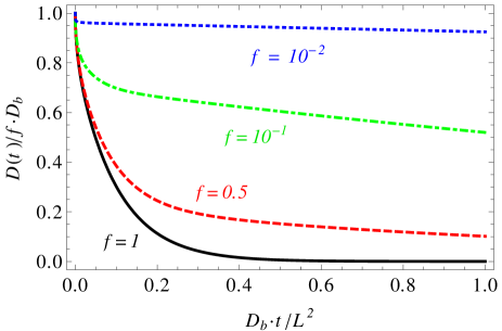
Figure 1: Time-dependent diffusion coefficient in reduced units as a function of the reduced time. Several ratios $f=(1+2k_{a}/k_{d}L)^{-1}$ are reported, which decrease with the strength of the sorption phenomena: (black line) $f=1$, i.e. without adsorption; (red dashed line) $f=0.5$; (green dot-dashed line) $f=10^{-1}$ and (blue dotted line) $f=10^{-2}$.

At $t=0$, $D(0)/D_{b}$ is simply the fraction $f=(1+2k_{a}/k_{d}L)^{-1}$ of mobile (non-adsorbed) particles. Figure 1 explores a large range of $f$, from weak to strong sorption. For all sorption parameters $k_{a}$ and $k_{d}$, diffusivity decreases with time, as increases the probability for each Brownian particle that explores the media to experience confinement by a wall and immobilization by adsorption. This decrease is strongly modified by the sorption processes, as the more probable it is for a particle to get adsorbed, the more time it takes to explore the media. At long times, because our media is not permeable, i.e. because the confinement is total in our geometry, the effective diffusion coefficient tends toward zero.

III Short and Long times Approximations

For $\frac{D_{b}}{k_{d}L^{2}}+\frac{k_{a}}{2k_{d}L}\gg 1$, i.e. for sufficiently long residence time on walls and fraction of adsorbed species, the series expansion of the hyperbolic functions in Eq. 16 allows, together with the residue theorem, to explicitely inverse Eq. 17 in the long time-limit (i.e. for $s\rightarrow 0$), leading to:

$$\frac{D_{\text{long}}\left(t\right)}{D_{b}}=f\times\frac{k_{a}L}{2D_{b}+k_{a}L}e^{\displaystyle-\frac{k_{d}}{1+\frac{k_{a}L}{2D_{b}}}t}.$$ (18)

At short times, we analytically inverse the power series expansion for $\mathcal{L}^{-1}\left[\lim_{s\rightarrow\infty}D\left(s\right)\right]$. The first terms read:

$$\frac{D_{\text{short}}(t)}{D_{b}}=f\times\left(1-\frac{4}{\sqrt{\pi}}\frac{\sqrt{D_{b}t}}{L}+2\frac{k_{a}t}{L}\right)+\mathcal{O}\left(t^{\frac{3}{2}}\right).$$ (19)

See Supplementary Material Document No. si for terms up to order 10 of the expansion. Figure 2 compares the short and long time approximations of the time-dependent diffusion coefficient to the full numerical inversion of the Laplace transform of Eq. 17 for $f=10^{-1}$. Together, the short and long time approximations provide a simple uniform approximation over the whole temporal domain.

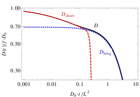
Figure 2: Reduced diffusion coefficient as a function of reduced time for $f=10^{-1}$; (black) from the full expression of Eq. 17, (red dashed line) from the short time approximation of Eq. 19 up to order 10 and (blue dotted line) from the long time approximation of Eq. 18.

IV Conclusion

In summary, we addressed explicitely the effect of adsorption and desorption phenomena on the time-dependent diffusion coefficient of Brownian particles confined between walls. The full expression of $D(t)$ is given, together with convenient and accurate approximations. It is shown that adsorption and desorption processes strongly modify $D(t)$, so that their consideration is important for proper determination of micro-geometric information from $D(t)$ measurements. Eq. 17 may also be used to extract sorption rates $k_{a}$ and $k_{d}$ from experimental measurements of $D(t)$, e.g. by PGSE-NMR. Finally, in more complex geometries, resort to numerical simulations such as Lattice BoltzmannRotenberg et al. (2008, 2010) is necessary. The present work provides exact reference results required for the validation of such numerical schemes in the presence of adsorption and desorption.