Explicit-Value Analysis
Based on CEGAR and Interpolation

Abstract

Abstraction, counterexample-guided refinement, and interpolation are techniques that are essential to the success of predicate-based program analysis. These techniques have not yet been applied together to explicit-value program analysis. We present an approach that integrates abstraction and interpolation-based refinement into an explicit-value analysis, i.e., a program analysis that tracks explicit values for a specified set of variables (the precision). The algorithm uses an abstract reachability graph as central data structure and a path-sensitive dynamic approach for precision adjustment. We evaluate our algorithm on the benchmark set of the Competition on Software Verification 2012 (SV-COMP’12) to show that our new approach is highly competitive. In addition, we show that combining our new approach with an auxiliary predicate analysis scores significantly higher than the SV-COMP’12 winner.

I Introduction

Abstraction is one of the most important techniques to successfully verify industrial-scale program code, because the abstract model omits details about the concrete semantics of the program that are not necessary to prove or disprove the program’s correctness. Counterexample-guided abstraction refinement (CEGAR) [14] is a technique that iteratively refines an abstract model using counterexamples. A counterexample is a witness of a property violation. In software verification, the counterexamples are error paths, i.e., paths through the program that violate the property. CEGAR starts with the most abstract model and checks if an error path can be found. If the analysis of the abstract model does not find an error path, then the analysis terminates, reporting that no violation exists. If the analysis finds an error path, the path is checked for feasibility, i.e., if the path is executable according to the concrete program semantics. If the error path is feasible, the analysis terminates, reporting the violation of the property, together with the feasible error path as witness. If the error path is infeasible, the violation is due to a too coarse abstract model and the infeasible error path is used to automatically refine the current abstraction. Then the analysis proceeds. Several successful tool implementations for software verification are based on abstraction and CEGAR (cf. [4, 6, 13, 16, 25, 10]). Craig interpolation is a technique from logics that yields for two contradicting formulas an interpolant that contains less information than the first formula, but still enough to contradict the second formula [17]. In software verification, interpolation can be used to extract information from infeasible error paths [21], where the resulting interpolants are used to refine the abstract model. Predicate abstraction is a successful abstraction technique for software model checking [18], because its symbolic state representation blends well with strongest post-conditions, and abstractions can be computed efficiently with solvers for satisfiability modulo theories (SMT) [3]. CEGAR and lazy refinement [22] together with interpolation [21] effectively refine abstract models in the predicate domain. The recent competition on software verification (SV-COMP’12 [5], Table 3) shows that these advancements had a strong impact on the success of participating tools (cf. [6, 10, 25, 26]).

Despite the success of abstraction, CEGAR, and interpolation in the field of predicate analysis, these techniques have not yet been combined and applied together to explicit-value analysis. We integrate these three techniques into an explicit-value analysis, a rather unsophisticated analysis that tracks for each program variable its current value explicitly (like constant propagation [1], but without join). First, we have to define the notion of abstraction for the explicit-value domain, and the precision of the analysis (i.e., the level of abstraction) by a set of program variables that the analysis has to track. Second, in order to automatically determine the necessary precision (i.e., a small set of program variables that need to be tracked) we use CEGAR iterations to discover finer precisions from infeasible error paths. Third, we define interpolation for the explicit-value domain and use this idea to construct an algorithm that efficiently extracts such a parsimonious precision that is sufficient to eliminate infeasible error paths.

Example. Consider the simple example program in Fig. 1. This program contains a $while$ loop in which a system call occurs. The loop exits if either the system call returns $0$ or a previously specified number of iterations $x$ was performed. Because the body of the function $system\_call$ is unknown, the value of $result$ is unknown. Also, the assumption $[ticks>x]$ cannot be evaluated to $true$, because $x$ is unknown. This program is correct, i.e., the error location in line 10 is not reachable. However, a simple explicit-value model checker that always tracks every variable would unroll the loop, always discovering new states, as the expression $ticks=ticks+1$ repeatedly assigns new values to variable $ticks$. Thus, due to extreme resource consumptions, the analysis would not terminate within practical time and memory limits, and is bound to give up on proving the safety property, eventually.

⬇

1extern int system_call();

2int main(int x) {

3 int flag, ticks, result;

4 flag = 0; ticks = 0;

5 while(1) {

6 ticks = ticks + 1;

7 result = system_call();

8 if(result == 0 || ticks > x) { break; }

9 }

10 if (flag > 0) { ERROR: return 1; }

11}

Figure 1: Example program to illustrate the effectiveness of CEGAR-based explicit-value analysis

The new approach for explicit-value analysis that we propose can efficiently prove this program safe, because it tracks only those variables that are necessary to refute the infeasible error paths. In the first CEGAR iteration, the precision of the analysis is empty, i.e., no variable is tracked. Thus, the error location will be reached. Now, using our interpolation-inspired method to discover precisions from counterexample paths, the algorithm identifies that the variable $flag$ (more precisely, the constraint $flag=0$) has to be tracked. The analysis is re-started after this refinement. Because $ticks$ is not in the precision (the variable is not tracked), the assignment $ticks=ticks+1$ will not add new abstract states. Since no new successors are computed, the analysis stops unrolling the loop. The assume operation $[flag>0]$ is evaluated to ${\it false}$, and thus, the error label is not reachable. The analysis terminates, proving the program correct.

In summary, the crucial effect of this approach is that only relevant variables are tracked in the analysis, while unimportant information is ignored. This greatly reduces the number of abstract states to be visited.

Contributions. We make the following contributions:

• We integrate the concepts of abstraction, CEGAR, and lazy abstraction refinement into explicit-value analysis.

• Inspired by Craig interpolation for predicate analysis, we define a novel interpolation-like approach for discovering relevant variables for the explicit-value domain. This refinement algorithm is completely self-contained, i.e., independent from external libraries such as SMT solvers.

• To further improve the effectiveness and efficiency of the analysis, we design a combination with a predicate analysis based on dynamic precision adjustment [9].

• We provide an open-source implementation of all our concepts and give evidence of the significant improvements by evaluating several approaches on benchmark verification tasks (C programs) from SV-COMP’12.

Related Work. The explicit-state model checker Spin [23] can verify models of programs written in a language called Promela. For the verification of C programs, tools like Modex  can extract Promela models from C source code. This process requires to give a specification of the abstraction level (user-defined extraction rules), i.e., the information of what should be included in the Promela model. Spin does not provide lazy-refinement-based CEGAR. Java PathFinder [20] is an explicit-state model checker for Java programs. There has been work [24] on integrating CEGAR into Java PathFinder, using an approach different from interpolation.

Program analysis with dynamic precision adjustment [9] is an approach to adjust the precision of combined analyses on-the-fly, i.e., during the analysis run; the precision of one analysis can be increased based on a current situation in another analysis. For example, if an explicit-value analysis stores too many different values for a variable, then the dynamic precision adjustment can remove that variable from the precision of the explicit-value analysis and add a predicate about that variable to the precision of a predicate analysis. This means that the tracking of the variable is “moved” from the explicit domain to the symbolic domain. One configuration that we present later in this paper uses this approach (cf. III-F).

The tool Dagger [19] improves the verification of C programs by applying interpolation-based refinement to octagon and polyhedra domains. To avoid imprecision due to widening in the join-based data-flow analysis, Dagger replaces the standard widen operator by a so called interpolated-widen operator, which increases the precision of the data-flow analysis and thus avoids false alarms. The algorithm Vinta [2] applies interpolation-based refinement to interval-like abstract domains. If the state exploration finds an error path, then Vinta performs a feasibility check using bounded model checking (BMC), and if the error path is infeasible, it computes interpolants. The interpolants are used to refine the invariants that the abstract domain operates on. Vinta requires an SMT solver for feasibility checks and interpolation.

More tools are mentioned in our evaluation section, where we compare (in terms of precision and efficiency) our tool implementation with tools that participated in SV-COMP’12.

There is, to the best of our knowledge, no work that integrates abstraction, CEGAR, lazy refinement, and interpolation into explicit-state model checking. We make those techniques available for the explicit-value domain.

II Preliminaries

Our approach is based on several existing concepts, and in this section we remind the reader of some basic definitions.

II-A Programs, Control-Flow Automata, States

We restrict the presentation to a simple imperative programming language, where all operations are either assignments or assume operations, and all variables range over integers . The following definitions are taken from previous work [11]: A program is represented by a control-flow automaton CFA. A CFA $A=(\mathit{L},G)$ consists of a set $\mathit{L}$ of program locations, which model the program counter, and a set $G\subseteq\mathit{L}\times Ops\times\mathit{L}$ of control-flow edges, which model the operations that are executed when control flows from one program location to another. The set of program variables that occur in operations from $Ops$ is denoted by $X$. A verification problem ${P=(A,{\mathit{l}_{0}},{\mathit{l}_{e}})}$ consists of a CFA $A$, representing the program, an initial program location ${\mathit{l}_{0}}\in\mathit{L}$, representing the program entry, and a target program location ${\mathit{l}_{e}}\in\mathit{L}$, which represents the error.

A concrete data state of a program is a variable assignment $cd:X\to\mathbb{Z}$, which assigns to each program variable an integer value. A concrete state of a program is a pair $(l,cd)$, where $l\in\mathit{L}$ is a program location and $cd$ is a concrete data state. The set of all concrete states of a program is denoted by ${\cal C}$, a subset $r\subseteq{\cal C}$ is called region. Each edge $g\in G$ defines a labeled transition relation $\mathord{\smash{\stackrel{{\scriptstyle g}}{{\rightarrow}}}}\subseteq{\cal C}\times\{g\}\times{\cal C}$. The complete transition relation $\smash{\stackrel{{\scriptstyle}}{{\rightarrow}}}$ is the union over all control-flow edges: $\mathord{\smash{\stackrel{{\scriptstyle}}{{\rightarrow}}}}=\bigcup_{g\in G}\smash{\stackrel{{\scriptstyle g}}{{\rightarrow}}}$. We write $c\smash{\stackrel{{\scriptstyle g}}{{\rightarrow}}}c^{\prime}$ if $(c,g,c^{\prime})\in\mathord{\smash{\stackrel{{\scriptstyle}}{{\rightarrow}}}}$, and $c\smash{\stackrel{{\scriptstyle}}{{\rightarrow}}}c^{\prime}$ if there exists a $g$ with $c\smash{\stackrel{{\scriptstyle g}}{{\rightarrow}}}c^{\prime}$.

An abstract data state represents a region of concrete data states, formally defined as abstract variable assignment. An abstract variable assignment is a partial function ${v:X\mathrel{\longrightarrow\circ\hskip 5.69054pt}\mathbb{Z}\cup\{\top,\bot\}}$, which maps variables in the definition range of function $v$ to integer values or $\top$ or $\bot$. The special value $\top$ is used to represent an unknown value, e.g., resulting from an uninitialized variable or an external function call, and the special value $\bot$ is used to represent no value, i.e., a contradicting variable assignment. We denote the definition range for a partial function $f$ as ${\textrm{def}(f)=\{x\mid\exists y:(x,y)\in f\}}$, and the restriction of a partial function $f$ to a new definition range $Y$ as $f_{|Y}={f\cap(Y\times(\mathbb{Z}\cup\{\top,\bot\}))}$. An abstract variable assignment $v$ represents the region $[\![v]\!]$ of all concrete data states $cd$ for which $v$ is valid, formally: $[\![v]\!]={\{cd\mid\forall x\in\textrm{def}(v):cd(x)=v(x)}$ or $v(x)=\top\}$. An abstract state of a program is a pair $(l,v)$, representing the following set of concrete states: $\{(l,cd)\mid cd\in[\![v]\!]\}$.

II-B Configurable Program Analysis with
Dynamic Precision Adjustment

We use the framework of configurable program analysis (CPA) [8], extended by the concept of dynamic precision adjustment [9]. Such a CPA supports adjusting the precision of an analysis during the exploration of the program’s abstract state space. A composite CPA can control the precision of its component analyses during the verification process, i.e., it can make a component analysis more abstract, and thus more efficient, or it can make a component analysis more precise, and thus more expensive. A CPA $\mathbb{D}=(D,\Pi,\smash{\stackrel{{\scriptstyle}}{{\rightsquigarrow}}},\mathsf{merge},\mathsf{stop},\mathsf{prec})$ consists of (1) an abstract domain $D$, (2) a set $\Pi$ of precisions, (3) a transfer relation $\smash{\stackrel{{\scriptstyle}}{{\rightsquigarrow}}}{}$, (4) a merge operator $\mathsf{merge}$, (5) a termination check $\mathsf{stop}$, and (6) a precision adjustment function $\mathsf{prec}$. Based on these components and operators, we can formulate a flexible and customizable reachability algorithm, which is adapted from previous work [8, 12].

II-C Explicit-Value Analysis as CPA

In the following, we define a component CPA that tracks explicit integer values for program variables. In order to obtain a complete analysis, we construct a composite CPA that consists of the component CPA for explicit values and another component CPA for tracking the program locations (CPA for location analysis, as previously described [9]). For the composite CPA, the general definitions of the abstract domain, the transfer relation, and the other operators are given in previous work [9]; the composition is done automatically by the framework implementation CPAchecker.

The CPA for explicit-value analysis, which tracks integer values for the variables of a program explicitly, is defined as $\mathbb{C}=(D_{\mathbb{C}},\Pi_{\mathbb{C}},\smash{\stackrel{{\scriptstyle}}{{\rightsquigarrow}}}_{\mathbb{C}},\mathsf{merge}_{\mathbb{C}},\mathsf{stop}_{\mathbb{C}},\mathsf{prec}_{\mathbb{C}})$ and consists of the following components [9]:

1. The abstract domain $D_{\mathbb{C}}=(C,\mathcal{V},[\![\cdot]\!])$ contains the set $C$ of concrete data states, and uses the semi-lattice $\mathcal{V}={(V,\top,\bot,\sqsubseteq,\sqcup)}$, which consists of the set $V=(X\mathrel{\longrightarrow\circ\hskip 5.69054pt}\mathcal{Z})$ of abstract variable assignments, where $\mathcal{Z}=\mathbb{Z}\cup\{\top_{\mathcal{Z}},\bot_{\mathcal{Z}}\}$ induces the flat lattice over the integer values (we write $\mathbb{Z}$ to denote the set of integer values). The top element $\top\in V$, with ${\top(x)=\top_{\mathcal{Z}}}$ for all $x\in X$, is the abstract variable assignment that holds no specific value for any variable, and the bottom element $\bot\in V$, with $\bot(x)=\bot_{\mathcal{Z}}$ for all $x\in X$, is the abstract variable assignment which models that there is no value assignment possible, i.e., a state that cannot be reached in an execution of the program. The partial order $\mathord{\sqsubseteq}\subseteq V\times V$ is defined as ${v\sqsubseteq v^{\prime}}$ if for all $x\in X$, we have $v(x)=v^{\prime}(x)$ or $v(x)=\bot_{\mathcal{Z}}$ or $v^{\prime}(x)=\top_{\mathcal{Z}}$. The join $\sqcup:V\times V\to V$ yields the least upper bound for two variable assignments. The concretization function ${[\![\cdot]\!]:V\to 2^{C}}$ assigns to each abstract data state $v$ its meaning, i.e., the set of concrete data states that it represents.

2. The set of precisions $\Pi_{\mathbb{C}}=2^{X}$ is the set of subsets of program variables. A precision $\pi\in\Pi_{\mathbb{C}}$ specifies a set of variables to be tracked. For example, $\pi=\emptyset$ means that no variable is tracked, and $\pi=X$ means that every program variable is tracked.

3. The transfer relation $\smash{\stackrel{{\scriptstyle}}{{\rightsquigarrow}}}_{\mathbb{C}}$ has the transfer $v\smash{\stackrel{{\scriptstyle g}}{{\rightsquigarrow}}}(v^{\prime},\pi)$ if
(1) $g=(\cdot,\mathtt{assume}(p),\cdot)$ and for all $x\in X:$
$v^{\prime}(x)=\left\{\begin{array}[]{ll}\bot_{\mathcal{Z}}&\text{if }(y,\bot_{\mathcal{Z}})\in v\text{ for some }y\in X\\ &\text{ or the formula }{p_{/v}}\text{ is unsatisfiable}\\ c&\text{if }c\text{ is the only satisfying assignment of}\\ &\text{ the formula }{p_{/v}}\text{ for variable }x\\ \top_{\mathcal{Z}}&\text{otherwise}\end{array}\right.$
where ${p_{/v}}$ denotes the interpretation of a predicate $p$ over variables from $X$ for an abstract variable assignment $v$, that is, ${p_{/v}}=\\ p~{}\land~{}\bigwedge\limits_{x\in\textrm{def}(v),v(x)\in\mathbb{Z}}x=v(x)~{}\land~{}\lnot\exists x\in\textrm{def}(v):v(x)=\bot_{\mathcal{Z}}$
or
(2) $g=(\cdot,\mathtt{w:=\,}exp,\cdot)$ and for all $x\in X:$
$v^{\prime}(x)=\left\{\begin{array}[]{ll}{exp_{/v}}&\text{if }x=\mathtt{w}\\ v(x)&\text{if }x\in\textrm{def}(v)\\ \top_{\mathcal{Z}}&\text{otherwise}\end{array}\right.$
where ${exp_{/v}}$ denotes the interpretation of an expression $exp$ over variables from $X$ for an abstract value assignment $v$:
${exp_{/v}}=\left\{\begin{array}[]{ll}\bot_{\mathcal{Z}}&\text{if }(y,\bot_{\mathcal{Z}})\in v\text{ for some }y\in X\\ \top_{\mathcal{Z}}&\text{if }(y,\top_{\mathcal{Z}})\in v\text{ or }y\not\in\textrm{def}(v)\\ &\text{ for some }y\in X\text{ that occurs in }exp\\ c&\text{otherwise, where expression $exp$}\\ &\text{ evaluates to $c$ after replacing each}\\ &\text{ occurrence of variable~{}$x$ with $x\in\textrm{def}(v)$ }\\ &\text{ by~{}$v(x)$ in $exp$ }\end{array}\right.$

4. The merge operator does not combine elements when control flow meets: $\mathsf{merge}_{\mathbb{C}}(v,v^{\prime},\pi)=v^{\prime}$.

5. The termination check considers abstract states individually: $\mathsf{stop}_{\mathbb{C}}(v,R,\pi)=(\exists v^{\prime}\in R:v\sqsubseteq v^{\prime})$.

6. The precision adjustment function computes a new abstract state with precision based on the abstract state $v$ and the precision $\pi$ by restricting the variable assignment $v$ to those variables that appear in $\pi$, formally: $\mathsf{prec}(v,\pi,R)=(v_{|\pi},\pi)$. (In this analysis instance, $\mathsf{prec}$ only adjusts the abstract state according to the current precision $\pi$, and leaves the precision itself unchanged.)

The precision of the analysis controls which program variables are tracked in an abstract state. In other approaches, this information is hard-wired in either the abstract-domain elements or the algorithm itself. The concept of CPA supports different precisions for different abstract states. A simple analysis can start with an initial precision and propagate it to new abstract states, such that the overall analysis uses a globally uniform precision. It is also possible to specify a precision individually per program location, instead of using one global precision. Our refinement approach in the next section will be based on location-specific precisions.

II-D Predicate Analysis as CPA

The abstract domain of predicates [18] was successfully used in several tools for software model checking (e.g., [4, 6, 13, 16, 25, 10]). In a predicate analysis, the precision is defined as a set of predicates, and the abstract states track the strongest set of predicates that are fulfilled (cartesian predicate abstraction) or the strongest boolean combination of predicates that are fulfilled (boolean predicate abstraction). This means, the abstraction level of the abstract model is determined by predicates that are tracked in the analysis. Predicate analysis is also implemented as a CPA in the framework CPAchecker, and a detailed description is available [11]. The precision is freely adjustable also in the predicate analysis, and we use this feature later in this article to compose a combined analysis. This analysis uses the predicate analysis to track variables that have many distinct values — a scenario in which the explicit-value analysis alone would be inefficient. The combined analysis adjusts the overall precision by removing variables with many distinct values from the precision of the explicit-value analysis and adds predicates about these variables to the precision of the predicate analysis [9] to allow the combined analysis to run efficiently.

II-E Lazy Abstraction

The concept of lazy abstraction [22] consists of two ideas: First, the abstract reachability graph (ARG) —the unfolding of the control-flow graph, representing our central data structure to store abstract states— is constructed on-the-fly, i.e., only when needed and only for parts of the state space that are reachable. We implement this using the standard reachability algorithm for CPAs as described in the next subsection. Second, the abstract states in the ARG are refined only where necessary along infeasible error paths in order to eliminate those paths. This is implemented by using CPAs with dynamic precision adjustment, where the refinement procedure operates on location-specific precisions and where the precision-adjustment operator always removes unnecessary information from abstract states, as outlined above.

II-F Reachability Algorithm for CPA

Algorithm 1 keeps updating two sets of abstract states with precision: the set $\mathsf{reached}$ to store all abstract states with precision that are found to be reachable, and a set $\mathsf{waitlist}$ to store all abstract states with precision that are not yet processed, i.e., the frontier. The state exploration starts with choosing and removing an abstract state with precision from the $\mathsf{waitlist}$, and the algorithm considers each abstract successor according to the transfer relation. Next, for the successor, the algorithm adjusts the precision of the successor using the precision adjustment function $\mathsf{prec}$. If the successor is a target state (i.e., a violation of the property is found), then the algorithm terminates, returning the current sets $\mathsf{reached}$ and $\mathsf{waitlist}$ — possibly as input for a subsequent precision refinement, as shown below (cf. Alg. 2). Otherwise, using the given operator $\mathsf{merge}$, the abstract successor state is combined with each existing abstract state from $\mathsf{reached}$. If the operator $\mathsf{merge}$ has added information to the new abstract state, such that the old abstract state is subsumed, then the old abstract state with precision is replaced by the new abstract state with precision in the sets $\mathsf{reached}$ and $\mathsf{waitlist}$. If after the merge step the resulting new abstract state with precision is covered by the set $\mathsf{reached}$, then further exploration of this abstract state is stopped. Otherwise, the abstract state with its precision is added to the set $\mathsf{reached}$ and to the set $\mathsf{waitlist}$. Finally, once the set $\mathsf{waitlist}$ is empty, the set $\mathsf{reached}$ is returned.

Algorithm 1 $\textsf{CPA}(\mathbb{D},R_{0},W_{0})$, adapted from [9]

0:  a CPA $\mathbb{D}=(D,\Pi,\smash{\stackrel{{\scriptstyle}}{{\rightsquigarrow}}},\mathsf{merge},\mathsf{stop},\mathsf{prec})$,       a set $R_{0}\subseteq(E\times\Pi)$ of abstract states with precision,       a subset $W_{0}\subseteq R_{0}$ of frontier abstract states with precision,       where $E$ denotes the set of elements of the semi-lattice of $D$

0:  a set of reachable abstract states with precision,        a subset of frontier abstract states with precision

0:  two sets $\mathsf{reached}$ and $\mathsf{waitlist}$ of elements of $E\times\Pi$

  $\mathsf{reached}:=R_{0}$; $\mathsf{waitlist}:=W_{0}$;

  while $\mathsf{waitlist}\not=\emptyset$ do

    choose $(e,\pi)$ from $\mathsf{waitlist}$; remove $(e,\pi)$ from $\mathsf{waitlist}$;

    for each $e^{\prime}$ with $e\smash{\stackrel{{\scriptstyle}}{{\rightsquigarrow}}}(e^{\prime},\pi)$ do

       // Precision adjustment.

       $(\hat{e},\hat{\pi}):=\mathsf{prec}(e^{\prime},\pi,\mathsf{reached})$;

       if $\mathsf{isTargetState}(\hat{e})$ then

          return $\big{(}\mathsf{reached}\cup(\hat{e},\hat{\pi}),\mathsf{waitlist}\big{)}$;

       for each $(e^{\prime\prime},\pi^{\prime\prime})\in\mathsf{reached}$ do

          // Combine with existing abstract state.

          $e_{new}:=\mathsf{merge}(\hat{e},e^{\prime\prime},\hat{\pi})$;

          if $e_{new}\not=e^{\prime\prime}$ then

             $\mathsf{waitlist}:=\big{(}\mathsf{waitlist}\cup\{(e_{new},\hat{\pi})\}\big{)}\setminus\{(e^{\prime\prime},\pi^{\prime\prime})\}$;

             $\mathsf{reached}:=\big{(}\mathsf{reached}\cup\{(e_{new},\hat{\pi})\}\big{)}\setminus\{(e^{\prime\prime},\pi^{\prime\prime})\}$;

       // Add new abstract state?

       if $\lnot~{}\mathord{\mathsf{stop}}\big{(}\hat{e},\big{\{}e\mid(e,\cdot)\in\mathsf{reached}\big{\}},\hat{\pi}\big{)}$ then

          $\mathsf{waitlist}:=\mathsf{waitlist}\cup\{(\hat{e},\hat{\pi})\}$; $\mathsf{reached}:=\mathsf{reached}\cup\{(\hat{e},\hat{\pi})\}$

  return $(\mathsf{reached},\emptyset)$;

II-G Counterexample-Guided Abstraction Refinement

Counterexample-guided abstraction refinement (CEGAR) [14] is a technique for automatic stepwise refinement of an abstract model. CEGAR is based on three concepts: (1) a precision, which determines the current level of abstraction, (2) a feasibility check, deciding if an abstract error path is feasible, i.e., if there exists a corresponding concrete error path, and (3) a refinement procedure, which takes as input an infeasible error path and extracts a precision that suffices to instruct the exploration algorithm to not explore the same path again later. Algorithm 2 shows an outline of a generic and simple CEGAR algorithm. The algorithm starts checking a program using a coarse initial precision $\pi_{0}$. It uses the reachability algorithm Alg. 1 for computing the reachable abstract state space, returning the sets $\mathsf{reached}$ and $\mathsf{waitlist}$. If the analysis has exhaustively checked all program states and did not reach the error, indicated by an empty set $\mathsf{waitlist}$, then the algorithm terminates and reports that the program is safe. If the algorithm finds an error in the abstract state space, i.e., a counterexample for the given specification, then the exploration algorithm stops and returns the unfinished, incomplete sets $\mathsf{reached}$ and $\mathsf{waitlist}$. Now the according abstract error path is extracted from the set $\mathsf{reached}$ using procedure $\mathsf{extractErrorPath}$ and analyzed for feasibility using the procedure $\mathsf{isFeasible}$ for feasibility check. If the abstract error path is feasible, meaning there exists a corresponding concrete error path, then this error path represents a violation of the specification and the algorithm terminates, reporting a bug. If the error path is infeasible, i.e., not corresponding to a concrete program path, then the precision was too coarse and needs to be refined. The algorithm extracts certain information from the error path in order to refine the precision based on that information using the procedure $\mathsf{Refine}$ for refinement, which returns a precision $\pi$ that makes the analysis strong enough to refute the infeasible error path in further state-space explorations. The current precision is extended using the precision returned by the refinement procedure and the analysis is restarted with this refined precision. Instead of restarting from the initial sets for $\mathsf{reached}$ and $\mathsf{waitlist}$, we can also prune those parts of the ARG that need to be rediscovered with new precisions, and replace the precision of the leaf nodes in the ARG with the refined precision, and then restart the exploration on the pruned sets. Our contribution in the next section is to introduce new implementations for the feasibility check as well as for the refinement procedure.

Algorithm 2 $\textsf{CEGAR}(\mathbb{D},e_{0},\pi_{0})$

0:  a configurable program analysis with dynamic precision       adjustment $\mathbb{D}=(D,\Pi,\smash{\stackrel{{\scriptstyle}}{{\rightsquigarrow}}},\mathsf{merge},\mathsf{stop},\mathsf{prec})$,       an initial abstract state $e_{0}\in E$ with precision $\pi_{0}\in\Pi$,       where $E$ denotes the set of elements of the semi-lattice of $D$

0:     verification result $\mathit{{\sc safe}}$ or $\mathit{{\sc unsafe}}$

  Variables: a set $\mathsf{reached}$ of elements of $E\times\Pi$,            a set $\mathsf{waitlist}$ of elements of $E\times\Pi$,            an error path $\sigma=\langle(\mathit{op}_{1},\mathit{l}_{1}),...,(\mathit{op}_{n},\mathit{l}_{n})\rangle$

  $\mathsf{reached}:=\{(e_{0},\pi_{0})\}$; $\mathsf{waitlist}:=\{(e_{0},\pi_{0})\}$; $\pi:=\pi_{0}$;

  while $true$ do

    $(\mathsf{reached},\mathsf{waitlist}):=\textsf{{CPA}}(\mathbb{D},\mathsf{reached},\mathsf{waitlist})$;

    if $\mathsf{waitlist}=\emptyset$ then

       return $\mathit{{\sc safe}}$

    else

       $\sigma:=\mathsf{extractErrorPath}(\mathsf{reached})$;

       if $\mathsf{isFeasible}(\sigma)$ then  // error path is feasible: report bug

          return $\mathit{{\sc unsafe}}$

       else  // error path is not feasible: refine and restart

          $\pi:=\pi\cup\mathsf{Refine}(\sigma)$;

          $\mathsf{reached}:={(e_{0},\pi)}$; $\mathsf{waitlist}:={(e_{0},\pi)}$;

II-H Interpolation

For a pair of formulas $\varphi^{-}$ and $\varphi^{+}$ such that $\varphi^{-}\land\varphi^{+}$ is unsatisfiable, a Craig interpolant $\psi$ is a formula that fulfills the following requirements [17]:

1. the implication $\varphi^{-}\Rightarrow\psi$ holds,

2. the conjunction $\psi\land\varphi^{+}$ is unsatisfiable, and

3. $\psi$ only contains symbols that occur in both $\varphi^{-}$ and $\varphi^{+}$.

Such a Craig interpolant is guaranteed to exist for many useful theories, for example, the theory of linear arithmetic with uninterpreted functions, as implemented in some SMT solvers (e.g., MathSAT , SMTInterpol ).

CEGAR based on Craig interpolation has been proven successful in the predicate domain. Therefore, we investigate if this technique is also beneficial for explicit-value model checking. Interpolants from the predicate domain, which consist of path formulas, are not useful for the explicit domain. Hence, we need to develop a procedure to compute interpolants for the explicit domain, which we introduce in the following section.

III Refinement-Based Explicit-Value Analysis

The level of abstraction in our explicit-value analysis is determined by the precisions for abstract variable assignments over program variables. The CEGAR-based iterative refinement needs an extraction method to obtain the necessary precision from infeasible error paths. We use our novel notion of interpolation for the explicit domain to achieve this goal.

III-A Explicit-Value Abstraction

We now introduce some necessary operations on abstract variable assignments, the semantics of operations and paths, and the precision for abstract variable assignments and programs, in order to be able to concisely discuss interpolation for abstract variable assignments and constraint sequences.

The operations implication and conjunction for abstract variable assignments are defined as follows: implication for $v$ and $v^{\prime}$: $v\mathrel{\Rightarrow}v^{\prime}$ if $\textrm{def}(v^{\prime})\subseteq\textrm{def}(v)$ and for each variable $x\in\textrm{def}(v)\cap\textrm{def}(v^{\prime})$ we have $v(x)=v^{\prime}(x)$ or $v(x)=\bot$ or $v^{\prime}(x)=\top$; conjunction for $v$ and $v^{\prime}$: for each variable $x\in\textrm{def}(v)\cup\textrm{def}(v^{\prime})$ we have
$(v\land v^{\prime})(x)=\left\{\begin{array}[]{ll}v(x)&\textrm{if }x\in\textrm{def}(v)\textrm{ and }x\not\in\textrm{def}(v^{\prime})\\ v^{\prime}(x)&\textrm{if }x\not\in\textrm{def}(v)\textrm{ and }x\in\textrm{def}(v^{\prime})\\ v(x)&\textrm{if }v(x)=v^{\prime}(x)\\ \bot&\textrm{if }\top\not=v(x)\not=v^{\prime}(x)\not=\top\\ \top&\textrm{otherwise }(v(x)=\top\textrm{ or }v^{\prime}(x)=\top)\end{array}\right.$

Furthermore we define contradiction for an abstract variable assignment $v$: $v$ is contradicting if there is a variable $x\in\textrm{def}(v)$ such that $v(x)=\bot$ (which implies $[\![v]\!]=\emptyset$); and renaming for $v$: the abstract variable assignment $v^{x\mapsto y}$, with $y\not\in\textrm{def}(v)$, results from $v$ by renaming variable $x$ to $y$: $v^{x\mapsto y}=(v\setminus\{(x,v(x))\})\cup\{(y,v(x))\}$.

The semantics of an operation $\mathit{op}\in Ops$ is defined by the strongest post-operator ${\sf SP}_{\mathit{op}}({\cdot})$ for abstract variable assignments: given an abstract variable assignment $v$, ${\sf SP}_{\mathit{op}}({v})$ represents the set of data states that are reachable from any of the states in the region represented by $v$ after the execution of $\mathit{op}$. Formally, given an abstract variable assignment $v$ and an assignment operation $s:=exp$, we have ${\sf SP}_{s:=exp}({v})=v_{|{X\setminus\{s\}}}\land v_{s:=exp}$ with $v_{s:=exp}=\{(s,{exp_{/v}})\}$, where ${exp_{/v}}$ denotes the interpretation of expression $exp$ for the abstract variable assignment $v$ (cf. definition of ${exp_{/v}}$ in Subsection II-C). That is, the value of variable $s$ is the result of the arithmetic evaluation of expression $exp$, or $\top$ if not all values in the expression are known, or $\bot$ if no value is possible (an abstract data state in which a variable is assigned to $\bot$ does not represent any concrete data state). Given an abstract variable assignment $v$ and an assume operation ${[p]}$, we have ${\sf SP}_{[p]}({v})=v^{\prime}$ and for all $x\in X$ we have $v^{\prime}(x)=\bot$ if $(y,\bot)\in v$ for some variable $x\in X$ or the formula ${p_{/v}}$ is unsatisfiable, or $v^{\prime}(x)=c$ if c is the only satisfying assignment of the formula ${p_{/v}}$ for variable $x$, or $v^{\prime}(x)=\top$ in all other cases; the formula ${p_{/v}}$ is defined as in Subsection II-C.

A path $\sigma$ is a sequence $\langle(\mathit{op}_{1},\mathit{l}_{1}),...,(\mathit{op}_{n},\mathit{l}_{n})\rangle$ of pairs of an operation and a location. The path $\sigma$ is called program path if for every $i$ with $1\leq i\leq n$ there exists a CFA edge $g=(\mathit{l}_{i-1},\mathit{op}_{i},\mathit{l}_{i})$ and $\mathit{l}_{0}$ is the initial program location, i.e., $\sigma$ represents a syntactic walk through the CFA. Every path $\sigma=\langle(\mathit{op}_{1},\mathit{l}_{1}),...,(\mathit{op}_{n},\mathit{l}_{n})\rangle$ defines a constraint sequence ${\gamma}_{\sigma}=\langle\mathit{op}_{1},...,\mathit{op}_{n}\rangle$. The semantics of a program path $\sigma=\langle(\mathit{op}_{1},\mathit{l}_{1}),...,(\mathit{op}_{n},\mathit{l}_{n})\rangle$ is defined as the successive application of the strongest post-operator to each operation of the corresponding constraint sequence ${\gamma}_{\sigma}$: ${\sf SP}_{{\gamma}_{\sigma}}({v})={\sf SP}_{\mathit{op}_{n}}({...{\sf SP}_{\mathit{op}_{i}}({..{\sf SP}_{\mathit{op}_{1}}({v})..})...})$. The set of concrete program states that result from running $\sigma$ is represented by the pair $(l_{n},{\sf SP}_{{\gamma}_{\sigma}}({v_{0}}))$, where $v_{0}=\{\}$ is the initial abstract variable assignment that does not map any variable to a value. A program path $\sigma$ is feasible if ${\sf SP}_{{\gamma}_{\sigma}}({v_{0}})$ is not contradicting, i.e., ${\sf SP}_{{\gamma}_{\sigma}}({v_{0}})(x)\not=\bot$ for all variables $x$ in $\textrm{def}({\sf SP}_{{\gamma}_{\sigma}}({v_{0}}))$. A concrete state $(l_{n},cd_{n})$ is reachable from a region $r$, denoted by $(l_{n},cd_{n})\in Reach(r)$, if there exists a feasible program path $\sigma=\langle(\mathit{op}_{1},\mathit{l}_{1}),...,(\mathit{op}_{n},\mathit{l}_{n})\rangle$ with $(l_{0},v_{0})\in r$ and $cd_{n}\in[\![{\sf SP}_{{\gamma}_{\sigma}}({v_{0}})]\!]$. A location $l$ is reachable if there exists a concrete state $c$ such that $(l,c)$ is reachable. A program is safe if ${\mathit{l}_{e}}$ is not reachable.

The precision for an abstract variable assignment is a set $\pi$ of variables. The explicit-value abstraction for an abstract variable assignment is an abstract variable assignment that is defined only on variables that are in the precision $\pi$. For example, the explicit-value abstraction for the variable assignment ${v=\{x\mapsto 2,y\mapsto 5\}}$ and the precision $\pi=\{x\}$ is the abstract variable assignment $v^{\pi}=\{x\mapsto 2\}$.

The precision for a program is a function $\Pi:L\to 2^{X}$, which assigns to each program location a precision for an abstract variable assignment, i.e., a set of variables for which the analysis is instructed to track values. A lazy explicit-value abstraction of a program uses different precisions for different abstract states on different program paths in the abstract reachability graph (ARG). The explicit-value abstraction for a variable assignment at location $l$ is computed using the precision $\Pi(l)$.

III-B CEGAR for Explicit-Value Model Checking

We now instantiate the three components of the CEGAR technique, i.e., precision, feasibility check, and refinement, for our explicit-value analysis. The precisions that our CEGAR instance uses are the above introduced precisions for a program (which assign to each program location a set of variables), and we start the CEGAR iteration with the empty precision, i.e., $\Pi_{init}(l)=\emptyset$ for each $l\in L$, such that no variable will be tracked.

The feasibility check for a path $\sigma$ is performed by executing an explicit-value analysis of the path $\sigma$ using the full precision $\Pi(l)=X$ for all locations $l$, i.e., all variables will be tracked. This is equivalent to computing ${\sf SP}_{{\gamma}_{\sigma}}({v_{0}})$ and check if the result is contradicting, i.e., if there is a variable for which the resulting abstract variable assignment is $\bot$. This feasibility check is extremely efficient, because the path is finite and the strongest post-operations for abstract variable assignments are simple arithmetic evaluations. If the feasibility check reaches the error location ${\mathit{l}_{e}}$, then this error can be reported. If the check cannot reach the error location, because of a contradicting abstract variable assignment, then a refinement is necessary because at least one constraint depends on a variable that was not yet tracked.

We define the last component of the CEGAR technique, the refinement, after we introduced the notion of interpolation for variable assignments and constraint sequences.

III-C Interpolation for Variable Assignments

For each infeasible error path in the above mentioned refinement operation, we need to determine a precision that assigns to each program location on that path the set of program variables that the explicit-value analysis needs to track in order to eliminate that infeasible error path in future explorations. Therefore, we define an interpolant for abstract variable assignments.

An interpolant for a pair of abstract variable assignments $v^{-}$ and $v^{+}$, such that $v^{-}\land v^{+}$ is contradicting, is an abstract variable assignment ${\mathcal{V}}$ that fulfills the following requirements:

1. the implication $v^{-}\mathrel{\Rightarrow}{\mathcal{V}}$ holds,

2. the conjunction ${\mathcal{V}}\land v^{+}$ is contradicting, and

3. ${\mathcal{V}}$ only contains variables in its definition range which are in the definition ranges of both $v^{-}$ and $v^{+}$ ($\textrm{def}({\mathcal{V}})\subseteq\textrm{def}(v^{-})\cap\textrm{def}(v^{+})$).

Lemma. For a given pair $(v^{-}$, $v^{+})$ of abstract variable assignments, such that $v^{-}\land v^{+}$ is contradicting, an interpolant exists. Such an interpolant can be computed in time $O(m+n)$, where $m$ and $n$ are the sizes of $v^{-}$ and $v^{+}$, respectively.

Proof. The variable assignment $v^{-}_{|\textrm{def}(v^{+})}$ is an interpolant for the pair $(v^{-}$, $v^{+})$.

Note. The above-mentioned interpolant that simply results from restricting $v^{-}$ to the definition range of $v^{+}$ (common definition range) is of course not a ‘good’ interpolant. In practice, we strive for interpolants with minimal definition range, and use slightly more expensive algorithms to compute them. Interpolation for abstract variable assignments is a first idea to approach the problem, but since we need to extract interpolants for paths, we next define interpolation for constraint sequences.

III-D Interpolation for Constraint Sequences

A more expressive interpolation can be achieved by considering constraint sequences. The conjunction ${{\gamma}\land{\gamma}^{\prime}}$ of two constraint sequences ${{\gamma}=\langle\mathit{op}_{1},...,\mathit{op}_{n}\rangle}$ and ${\gamma}^{\prime}=\langle\mathit{op}_{1}^{\prime},...,\mathit{op}_{m}^{\prime}\rangle$ is defined as their concatenation, i.e., ${{\gamma}\land{\gamma}^{\prime}=\langle\mathit{op}_{1},...,\mathit{op}_{n},\mathit{op}_{1}^{\prime},...,\mathit{op}_{m}^{\prime}\rangle}$, the implication of ${\gamma}$ and ${\gamma}^{\prime}$ (denoted by ${\gamma}\mathrel{\Rightarrow}{\gamma}^{\prime}$) as ${\sf SP}_{{\gamma}}({v_{0}})\mathrel{\Rightarrow}{\sf SP}_{{\gamma}^{\prime}}({v_{0}})$, and ${\gamma}$ is contradicting if $[\![{\sf SP}_{{\gamma}}({v_{0}})]\!]=\emptyset$, with $v_{0}=\{\}$.

An interpolant for a pair of constraint sequences ${\gamma}^{-}$ and ${\gamma}^{+}$, such that ${\gamma}^{-}\land{\gamma}^{+}$ is contradicting, is a constraint sequence  ${\Gamma}$ that fulfills the following requirements:

1. the implication ${\gamma}^{-}\mathrel{\Rightarrow}{\Gamma}$ holds,

2. the conjunction ${\Gamma}\land{\gamma}^{+}$ is contradicting, and

3. ${\Gamma}$ contains in its constraints only variables that occur in the constraints of both ${\gamma}^{-}$ and ${\gamma}^{+}$.

Lemma. For a given pair $({\gamma}^{-}$, ${\gamma}^{+})$ of constraint sequences, such that ${\gamma}^{-}\land{\gamma}^{+}$ is contradicting, an interpolant exists. Such an interpolant is computable in time $O(m\cdot n)$, where $m$ and $n$ are the sizes of ${\gamma}^{-}$ and ${\gamma}^{+}$, respectively.

Algorithm 3 $\mathsf{Interpolate}({\gamma}^{-},{\gamma}^{+})$

0:  two constraint sequences ${\gamma}^{-}$ and ${\gamma}^{+}$,           with ${\gamma}^{-}\land{\gamma}^{+}$ is contradicting

0:  a constraint sequence ${\Gamma}$,            which is an interpolant for ${\gamma}^{-}$ and ${\gamma}^{+}$

0:  an abstract variable assignment $v$

  $v:={\sf SP}_{{\gamma}^{-}}({\emptyset})$

  for each $x\in\textrm{def}{(v)}$ do

    if ${\sf SP}_{{\gamma}^{+}}({v_{|\textrm{def}(v)\setminus\{x\}}})$ is contradicting then

       // $x$ is not relevant and should not occur in the interpolant

       $v:=v_{|\textrm{def}(v)\setminus\{x\}}$

  // construct the interpolating constraint sequence

  ${\Gamma}:=\langle\rangle$

  for each $x\in\textrm{def}{(v)}$ do

    // construct an assume constraint for $x$

    ${\Gamma}:={\Gamma}\land\langle[x=v(x)]\rangle$

  return ${\Gamma}$

Proof. Algorithm $\mathsf{Interpolate}$ (Alg. 3) returns an interpolant for two constraint sequences ${\gamma}^{-}$ and ${\gamma}^{+}$. The algorithm starts with computing the strongest post-condition for ${\gamma}^{-}$ and assigns the result to the abstract variable assignment $v$, which then may contain up to $m$ variables. Per definition, the strongest post-condition for ${\gamma}^{+}$ of variable assignment $v$ is contradicting. Next we try to eliminate each variable from $v$, by testing if removing it from $v$ makes the strongest post-condition for ${\gamma}^{+}$ of $v$ contradicting (each such test takes $n$ $\mathsf{SP}$ steps). If it is contradicting, the variable can be removed. If not, the variable is necessary to prove the contradiction of the two constraint sequences, and thus, should occur in the interpolant. Note that this keeps only variables in $v$ that occur in ${\gamma}^{+}$ as well. The rest of the algorithm constructs a constraint sequence from the variable assignment, in order to return an interpolating constraint sequence, which fulfills the three requirements of an interpolant. A naive implementation can compute such an interpolant in $O((m+n)^{3})$.

III-E Refinement Based on Explicit-Interpolation

The goal of our interpolation-based refinement for explicit-value analysis is to determine a localized precision that is strong enough to eliminate an infeasible error path in future explorations. This criterion is fulfilled by the property of interpolants. A second goal is to have a precision that is as weak as possible, by creating interpolants that have a definition range as small as possible, in order to be parsimonious in tracking variables and creating abstract states.

Algorithm 4 $\mathsf{Refine}(\sigma)$

0:  infeasible error path $\sigma=\langle(\mathit{op}_{1},\mathit{l}_{1}),...,(\mathit{op}_{n},\mathit{l}_{n})\rangle$

0:  precision $\Pi$

0:  interpolating constraint sequence ${\Gamma}$

  ${\Gamma}:=\langle\rangle$;

  $\Pi(\mathit{l}):=\emptyset$, for all program locations $\mathit{l}$;

  for $i:=1$ to $n-1$ do

    ${\gamma}^{+}:=\langle\mathit{op}_{i+1},...,\mathit{op}_{n}\rangle$

    // inductive interpolation

    ${\Gamma}:=\mathsf{Interpolate}({\Gamma}\land\mathit{op}_{i},{\gamma}^{+})$

    // extract variables from variable assignment that results from ${\Gamma}$

    $\Pi(\mathit{l}_{i}):=\big{\{}x\big{|}(x,z)\in{\sf SP}_{{\Gamma}}({\emptyset})$ and $\bot\not=z\not=\top\big{\}}$

  return $\Pi$

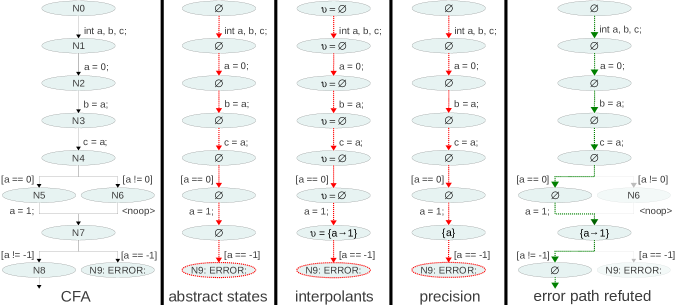
Figure 2: Illustration of one refinement iteration; from left to right: a simple example CFA, an infeasible error path with the abstract states annotated in the nodes (precision was empty, nothing is tracked), the interpolated variable assignments annotated in the nodes, the precisions extracted from the interpolants annotated in the nodes, and finally the CFA with the abstract states annotated in the nodes according to the new precision (unreached nodes —including error— shown in gray)

We apply the idea of interpolation for constraint sequences to assemble a precision-extraction algorithm: Algorithm $\mathsf{Refine}$ (Alg. 4) takes as input an infeasible program path, and returns a precision for a program. A further requirement is that the procedure computes inductive interpolants [6], i.e., each interpolant along the path contains just enough information to prove the remaining path infeasible. This is needed in order to ensure that the interpolants at the different locations achieve the goal of providing a precision that eliminates the infeasible error path from further explorations. For every program location $\mathit{l}_{i}$ along an infeasible error path $\sigma$, starting at $\mathit{l}_{0}$, we split the constraint sequence of the path into a constraint prefix ${\gamma}^{-}$, which consists of the constraints from the start location $l_{0}$ to $\mathit{l}_{i}$, and a constraint suffix ${\gamma}^{+}$, which consists of the path from the location $\mathit{l}_{i}$ to ${\mathit{l}_{e}}$. For computing inductive interpolants, we replace the constraint prefix by the conjunction of the last interpolant and the current constraint. The precision is extracted by computing the abstract variable assignment for the interpolating constraint sequence and assigning the relevant variables as precision for the current location $\mathit{l}_{i}$, i.e., the set of all variables that are necessary to be tracked in order to eliminate the error path from future exploration of the state space. This algorithm for precision extraction yields a parsimonious precision, i.e., a precision containing just enough information to exclude the infeasible error path, and can be directly plugged-in as refinement routine of the CEGAR algorithm (cf. Alg. 2). Note that the repetitive interpolations are not an efficiency bottleneck. The path is always finite, without any loops or branching, and thus, even a full-precision check can be decided efficiently. Figure 2 illustrates the interpolation process on a simple example.

III-F Optimizations

In our implementation, we added several optimizations to improve the performance of our approach.

ARG Pruning instead of Restart. Our refinement routine $\mathsf{Refine}$ (cf. Alg. 4) returns a set of variables (precision) that are important for deciding the reachability of the error location. One of the ideas of lazy abstraction refinement [22] is that the precision is only refined where necessary, i.e., only at the locations along the path that was considered in the refinement; the other parts of the state space are not refined. As mentioned in the discussion of the CEGAR algorithm (cf. Alg. 2), it is not necessary to restart the exploration of the state space from scratch after a refinement. Instead, we identify the descendant closest to the root of the abstract reachability graph (ARG) in which the precision was refined, and the re-exploration of the state space continues from there. In total, this significantly reduces the number of tracked variables per abstract state, which in turn leads to a more efficient analysis, because it drastically increases the chance that a new abstract state is covered by an existing abstract state.

Scoped Precision Refinement. The precision for a program assigns to each program location the set of variables that need to be tracked at that location, and the interpolation-based refinement adds new variables precisely at the locations for which they were discovered during refinement. In our experience, the number of refinements is reduced significantly if we add a variable to the precision not only at the particular location for which it was discovered, but at all locations in the local scope of the variable. This helps to avoid adding a variable twice that can occur on two different branches. By adding the variable to the precision “in advance” in the local scope, we abbreviate some refinement iterations. For example, consider Fig. 2 again. After the illustrated refinement, another refinement step would be necessary, in order to discover that variable $\mathsf{a}$ needs to be tracked at location $\mathsf{N4}$ as well (to prevent the analysis from going through location $\mathsf{N6}$). By adding variable $\mathsf{a}$ to the precision of all locations in the scope of variable $\mathsf{a}$ immediately after the first refinement, the program can be proved safe without further refinement. This effect was also observed, and used, in the software model checker Blast [6].

Precise Counterexample Check. In order to further increase the precision of our analysis, we double-check all feasible error paths using bit-precise bounded model checking (BMC) , by generating a path program [7] for the error path and let the BMC confirm the bug. Since the generated path program does not contain any loop or branching, it can be verified efficiently. If both our analysis and the bit-precise BMC report $\mathit{unsafe}$, then we report a bug. If the BMC cannot confirm the bug, our analysis continues trying to find another error path. This additional feature is available as a command-line option in our implementation.

Auxiliary Predicate Analysis. As an additional option for further improvement of the analysis, we implemented the combination with a predicate analysis, as outlined in existing work [9]. In this combination, if the explicit-value analysis finds an error path, this path is first checked for satisfiability in the predicate domain. If the satisfiability check is positive, the result $\mathit{unsafe}$ can be reported and the error path is returned; if negative, then the explicit-value domain is not expressive enough to analyze that program path (e.g., due to inequalities). In this case, we ask the predicate analysis to refine its abstraction along that path, which yields a refined predicate precision that eliminates the error path but considering the facts along that path in the (more precise, and more expensive) predicate domain. We need to parsimoniously use this feature because the post-operations of the predicate analysis are much more expensive than the post-operations of the explicit-value analysis. In general, after a refinement step, either the explicit-value precision is refined (preferred) or the predicate precision is refined (only if explicit does not succeed).

Using the concept of dynamic precision adjustment [9], we also switch off the tracking of variables in the explicit-value domain if the number of different values on a path exceeds a certain threshold. After this, the predicate analysis will get switched on (by the above-mentioned mechanism) and the facts on that path are further tracked using predicates. This is important if the explicit-value analysis tries to unwind loops; the symbolic, predicate-based analysis can often store a large number of values more efficiently.

Note that this refinement-based, parallel composition with precision adjustment of the explicit-value analysis and the predicate analysis is more powerful than a mere parallel product of the two analyses, because after each refinement, the explicit part of the analysis tracks exactly what it is capable of tracking, while the auxiliary predicate analysis takes care of only those facts that are beyond the capabilities of the explicit domain, resulting in a lightweight analysis on both ends. Such a combination is easy to achieve in our implementation, because we use the framework of configurable program analysis (CPA), which lets the user freely configure such combinations.

IV Experiments

In order to demonstrate that our approach yields a significant practical improvement of verification efficiency and effectiveness, we implemented our algorithms and compared our new techniques to existing tools for software verification. In the following, we show that the application of abstraction, CEGAR, and interpolation to the explicit-value domain considerably improves the number of solved instances and the run time. Combinations of the new explicit-value analysis with a predicate-based analysis can further increase the number of solved instances. All our experiments were performed on hardware identical to that of the SV-COMP’12 [5], such that our results are comparable to all the results obtained there.

Compared Verification Approaches. For presentation, we restrict the comparison of our new approach to the SV-COMP’12 participants Blast, SATabs, and the competition winner cpa-memo, all of which are based on predicate abstraction and CEGAR. Furthermore, to investigate performance differences in the same tool environment, we also compare with different configurations of CPAchecker. The model checker Blast is based on predicate abstraction, and uses a CEGAR loop for abstraction refinement. The predicates for the precision are learned from counterexample paths using interpolation. The central data structure of the algorithm is an ARG, which is lazily constructed and refined. Blast won the category “DeviceDrivers64” in the SV-COMP’12, and got bronze in another category. The model checker SATabs is also based on predicate abstraction and CEGAR, but in contrast to Blast, it constructs and checks in every iteration of the CEGAR loop a new boolean program based on the current precision of the predicate abstraction, and does not use lazy abstraction or interpolation. SATabs got silver in the categories “SystemC” and “Concurrency”, and bronze in another category. The model checker cpa-memo is based on predicate abstraction, CEGAR, and interpolation, but extends it with the concepts of adjustable-block encoding [11] and block-abstraction memoization [26]. cpa-memo won the category “Overall”, got silver in two more categories, and bronze in another category.

We implemented our concepts as extensions of CPAchecker [10], a software-verification framework based on configurable program analysis (CPA). We compare with the existing explicit-value analysis (without abstraction, CEGAR, and interpolation) and with the existing predicate analysis that is based on boolean predicate abstraction, CEGAR, interpolation, and adjustable-block encoding [11]. We used the trunk version of CPAchecker in revision 6615.

Verification Tasks. For the evaluation of our approach, we use all SV-COMP’12  verification tasks that do not involve concurrency properties (all categories except category “Concurrency”). All obtained experimental data as well as the tool implementation are available at http://www.sosy-lab.org/$\sim$dbeyer/cpa-explicit.

Quality Measures. We compare the verification results of all verification approaches based on three measures for verification quality: First, we take the run time, in seconds, of the verification runs to measure the efficiency of an approach. Obviously, the lower the run time, the better the tool. Second, we use the number of correctly solved instances of verification tasks to measure the effectiveness of an approach. The more instances a tool can solve, the more powerful the analysis is. Third, and most importantly, we use the scoring schema of the SV-COMP’12 as indicator for the quality of an approach. The scoring schema implements a community-agreed weighting schema, namely, that it is more difficult to prove a program correct compared to finding a bug and that a wrong answer should be penalized with double the scores that a correct answer would have achieved. For a full discussion of the official rules and benchmarks of the SV-COMP’12, we refer to the competition report [5]. Besides the data tables, we use plots of quantile functions [5] for visualizing the number of solved instances and the verification time. The quantile function for one approach contains all pairs $(x,y)$ such that the maximum run time of the $x$ fastest results is $y$. We use a logarithmic scale for the time range from 1 s to 1000 s and a linear scale for the time range between 0 s and 1 s. In addition, we decorate the graphs with symbols at every fifth data point in order to make the graphs distinguishable on gray-scale prints.

Category	cpa-expl			cpa-explitp
	points	solved	time	points	solved	time
ControlFlowInt	124	81	8400	123	79	780
DeviceDrivers	53	37	63	53	37	69
DeviceDrivers64	5	5	660	33	19	200
HeapManipul	1	3	5.5	1	3	5.8
SystemC	34	26	1600	34	26	1500
Overall 8	217	152	11000	244	164	2500

TABLE I: Comparison with purely explicit, non-CEGAR approach

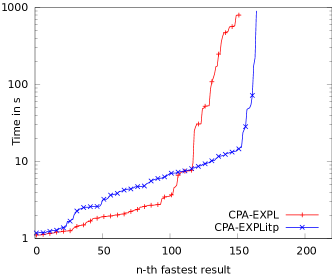
Figure 3: Quantile plot: purely explicit analyses

Improvements of Explicit-Value Analysis. In the first evaluation, we compare two different configurations of the explicit-value analysis: cpa-expl refers to the existing implementation of a standard explicit-value analysis without abstraction and refinement, and cpa-explitp refers to the new approach, which implements abstraction, CEGAR, and interpolation. Table I and Fig. 3 show that the new approach uses less time, solves more instances, and obtains more points in the SV-COMP’12 scoring schema.

Improvements of Combination with Predicate Analysis. In the second evaluation, we compare the refinement-based explicit analysis against a standard predicate analysis, as well as to the predicate analysis combined with cpa-expl and cpa-explitp, respectively: cpa-pred refers to a standard predicate analysis that CPAchecker offers (ABE-lf, [11]), cpa-explitp refers again to the explicit-value analysis, which implements abstraction, CEGAR, and interpolation, cpa-expl-pred refers to the combination of predicate analysis and explicit-value analysis without refinement, and cpa-explitp-pred refers to the combination of predicate analysis and explicit-value analysis with refinement.

Table IV and Fig. 4 show that the new combination approach outperforms the existing approaches cpa-pred and cpa-explitp in terms of solved instances and score. The comparison with column cpa-expl-pred is interesting because it shows that the combination of two analyses is an improvement even without refinement in the explicit-value analysis, but switching on the refinement in both domains makes the new combination significantly more effective.

Comparison with State-of-the-Art Verifiers. In the third evaluation, we compare our new combination approach with three established tools: Blast refers to the standard Blast configuration that participated in the SV-COMP’12, SATabs also refers to the respective standard configuration, cpa-memo refers to a special predicate abstraction that is based on block-abstraction memoization, and cpa-explitp-pred refers to our novel approach, which combines a predicate analysis (cpa-pred) with the new explicit-value analysis that is based on abstraction, CEGAR, and interpolation (cpa-explitp). Table IV and Fig. 5 show that the new approach outperforms Blast and SATabs by consuming considerably less verification time, more solved instances, and a better score. Even compared to the SV-COMP’12 winner, cpa-memo, our new approach scores higher. It is interesting to observe that the difference in scores is much higher than the difference in solved instances: this means cpa-memo had many incorrect verification results, which in turn shows that our new combination is significantly more precise.

Category	cpa-pred			cpa-explitp			cpa-expl-pred			cpa-explitp-pred
	score	solved	time	score	solved	time	score	solved	time	score	solved	time
ControlFlowInt	103	70	2500	123	79	780	131	85	2600	141	91	830
DeviceDrivers	71	46	80	53	37	69	71	46	82	71	46	87
DeviceDrivers64	33	24	2700	33	19	200	10	11	1100	37	24	980
HeapManipul	8	6	12	1	3	5.8	6	5	11	8	6	12
SystemC	22	17	1900	34	26	1500	62	45	1500	61	44	3700
Overall 8	237	163	7100	244	164	2500	280	192	5300	318	211

TABLE II: Comparison with predicate-based configurations

TABLE III: Comparison with three existing tools

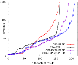
Figure 4: Quantile plot: comparison with predicate-based configurations

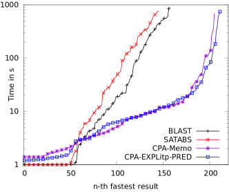
Figure 5: Quantile plot: comparison with three existing tools

V Conclusion

The surprising insight of this work is that it is possible to achieve —without using sophisticated SMT-solvers during the abstraction refinement— a performance and precision that can compete with the world’s leading symbolic model checkers, which are based on SMT-based predicate abstraction. We achieved this by incorporating the ideas of abstraction, counterexample-guided abstraction refinement, lazy abstraction refinement, and interpolation into a standard, simple explicit-value analysis.

We further improved the performance and precision by combining our refinement-based explicit-value analysis with a predicate analysis, in order to benefit from the complementary advantages of the methods. The combination analysis dynamically adjusts the precision [9] for an optimal trade-off between the precision of the explicit analysis and the precision of the auxiliary predicate analysis. This combination out-performs state-of-the-art model checkers, witnessed by a thorough comparison on a standardized set of benchmarks.

Despite the overall success of our new approach, individual instances of benchmarks show different performance with different configurations — i.e., either with or without CEGAR. Therefore, a general heuristic for finding a suitable strategy for a single verification task would be beneficial. Also, we envision better support for pointers and data structures, because our interpolation approach can be efficiently applied even with high precision. Moreover, we so far only combined our interpolation approach with an auxiliary predicate analysis in the ABE-lf configuration, and we have not yet tried to combine this with the superior block-abstraction memoization (ABM) [26] technique. Finally, we plan to extend our interpolation approach to other abstract domains like intervals.

References

- [1] A. V. Aho, R. Sethi, and J. D. Ullman. Compilers: Principles, Techniques, and Tools. Addison-Wesley, 1986.
- [2] A. Albarghouthi, A. Gurfinkel, and M. Chechik. Craig interpretation. In Proc. SAS, pages 300–316, 2012.
- [3] T. Ball, A. Podelski, and S. K. Rajamani. Boolean and cartesian abstractions for model checking C programs. In Proc. TACAS, LNCS 2031, pages 268–283. Springer, 2001.
- [4] T. Ball and S. K. Rajamani. The Slam project: Debugging system software via static analysis. In Proc. POPL, pages 1–3. ACM, 2002.
- [5] D. Beyer. Competition on Software Verification (SV-COMP). In Proc. TACAS, LNCS 7214, pages 504–524. Springer, 2012.
- [6] D. Beyer, T. A. Henzinger, R. Jhala, and R. Majumdar. The software model checker Blast. Int. J. Softw. Tools Technol. Transfer, 9(5-6):505–525, 2007.
- [7] D. Beyer, T. A. Henzinger, R. Majumdar, and A. Rybalchenko. Path programs. In Proc. PLDI, pages 300–309. ACM, 2007.
- [8] D. Beyer, T. A. Henzinger, and G. Théoduloz. Configurable software verification: Concretizing the convergence of model checking and program analysis. In Proc. CAV, LNCS 4590, pages 504–518. Springer, 2007.
- [9] D. Beyer, T. A. Henzinger, and G. Théoduloz. Program analysis with dynamic precision adjustment. In Proc. ASE, pages 29–38. IEEE, 2008.
- [10] D. Beyer and M. E. Keremoglu. CPAchecker: A tool for configurable software verification. In Proc. CAV, LNCS 6806, pages 184–190. Springer, 2011.
- [11] D. Beyer, M. E. Keremoglu, and P. Wendler. Predicate abstraction with adjustable-block encoding. In Proc. FMCAD, pages 189–197. FMCAD, 2010.
- [12] D. Beyer and P. Wendler. Algorithms for software model checking: Predicate abstraction vs. Impact. In Proc. FMCAD, pages 106–113. FMCAD, 2012.
- [13] S. Chaki, E. M. Clarke, A. Groce, S. Jha, and H. Veith. Modular verification of software components in C. IEEE Trans. Softw. Eng., 30(6):388–402, 2004.
- [14] E. M. Clarke, O. Grumberg, S. Jha, Y. Lu, and H. Veith. Counterexample-guided abstraction refinement for symbolic model checking. J. ACM, 50(5):752–794, 2003.
- [15] E. M. Clarke, D. Kröning, and F. Lerda. A tool for checking ANSI-C programs. In Proc. TACAS, LNCS 2988, pages 168–176. Springer, 2004.
- [16] E. M. Clarke, D. Kröning, N. Sharygina, and K. Yorav. SatAbs: SAT-based predicate abstraction for ANSI-C. In Proc. TACAS, LNCS 3440, pages 570–574. Springer, 2005.
- [17] W. Craig. Linear reasoning. A new form of the Herbrand-Gentzen theorem. J. Symb. Log., 22(3):250–268, 1957.
- [18] S. Graf and H. Saïdi. Construction of abstract state graphs with Pvs. In Proc. CAV, LNCS 1254, pages 72–83. Springer, 1997.
- [19] B. S. Gulavani, S. Chakraborty, A. V. Nori, and S. K. Rajamani. Automatically refining abstract interpretations. In Proc. TACAS, LNCS 4963, pages 443–458. Springer, 2008.
- [20] K. Havelund and T. Pressburger. Model checking Java programs using Java PathFinder. Int. J. Softw. Tools Technol. Transfer, 2(4):366–381, 2000.
- [21] T. A. Henzinger, R. Jhala, R. Majumdar, and K. L. McMillan. Abstractions from proofs. In Proc. POPL, pages 232–244. ACM, 2004.
- [22] T. A. Henzinger, R. Jhala, R. Majumdar, and G. Sutre. Lazy abstraction. In Proc. POPL, pages 58–70. ACM, 2002.
- [23] G. J. Holzmann. The Spin model checker. IEEE Trans. Softw. Eng., 23(5):279–295, 1997.
- [24] C. S. Pasareanu, M. B. Dwyer, and W. Visser. Finding feasible counter-examples when model checking abstracted Java programs. In Proc. TACAS, LNCS 2031, pages 284–298. Springer, 2001.
- [25] A. Podelski and A. Rybalchenko. Armc: The logical choice for software model checking with abstraction refinement. In Proc. PADL, LNCS 4354, pages 245–259. Springer, 2007.
- [26] D. Wonisch. Block abstraction memoization for CPAchecker. In Proc. TACAS, LNCS 7214, pages 531–533. Springer, 2012.