The dependence of topological Anderson insulator on the type of disorder

Abstract

This paper details the investigation of the influence of different disorders in two-dimensional topological insulator systems. Unlike the phase transitions to topological Anderson insulator induced by normal Anderson disorder, a different physical picture arises when bond disorder is considered. Using Born approximation theory, an explanation is given as to why bond disorder plays a different role in phase transition than does Anderson disorder. By comparing phase diagrams, conductance, conductance fluctuations, and the localization length for systems with different types of disorder, a consistent conclusion is obtained. The results indicate that a topological Anderson insulator is dependent on the type of disorder. These results are important for the doping processes used in preparation of topological insulators.

I Introduction

With research breakthroughs in HgTe/CdTe quantum wells and 3D topological materials, 1 (1, 2, 3, 4, 5, 6, 7) topological insulators have attracted much attention in recent years. These unique topological properties are responsible for some interesting and surprising phenomena. For example, in 2009, Li, Chu, Jain and Shen Shen (8) discovered that Anderson disorder can lead to a topological phase transitions with quantized conductance and named this phase topological Anderson insulator (TAI). The phenomenon of TAI was also reported by Jiang et al. Jiang (9) in their work. Subsequently, the origins of TAI, as well as TAI in other systems, have been studied by many groups using a variety of methods. Guo (10, 11, 12, 13, 14, 15, 16) Guo et al. Guo (10) found that the TAI phenomenon also exists in disordered 3D topological insulator. Recently, Xing et al. Xing (11) compared the disorder effects in three different systems where the quantum anomalous Hall effect exists. They observed TAI in these three different systems and demonstrated that increasing disorder strength produces the TAI phenomenon. Furthermore, Yamakage et al. Kuramoto (12) reported similar phase transitions in disordered $Z_{2}$ topological insulators when considering $s_{z}$ non-conserving spin-orbit coupling. The origins of TAI have been studied by many groups as well. After the initial reports of TAI, Shen (8) Jiang et al. Jiang (9) calculated the distribution of local currents in real space at various strengthes of Anderson disorder and provided an explanation on TAI phase by studying the helical edge states in HgTe/CdTe quantum wells. In addition, it has been shown by Groth et al. Beenakker (13) that the phase transition to TAI should ascribe to a negative correction to the topological mass because of Anderson disorder. Using the effective medium theory and through numerical calculations, Groth et al. Beenakker (13) discussed in detail how Anderson disorder renormalizes the topological mass, chemical potential and finally induces a phase transition. This interpretation provides a clear physical image of TAI and has been accepted generally by most physicists in this field. The TAI effect has also been identified in 3D topological insulators and the effective medium theory noted above is found to be useful when describing the 3D case as reported in the paper by Guo et al. Guo (10) However, by looking at the phase diagrams, Prodan Prodan (14) takes the position in his paper that TAI should not be considered a distinct phase but should be described as part of the quantum spin-Hall phase. In addition, Chen et al. Chen (15) discussed the TAI phenomenon from the point of band structures. Finally, by calculating the $Z_{2}$ topological number in systems with periodic disordered supercell regimes, Zhang et al. Zhang (16) verified that TAI corresponds to a topologically non-trivial phase. Thus, it has been well documented that Anderson disorder may induce TAI. However, it is not clear whether TAI is certain to be observed experimentally and whether all types of disorder can definitely push a phase transition to TAI for an anomalous quantum Hall system. It is the purpose of this paper to address these questions. Besides the on-site Anderson disorder, there exists another type of disorder, bond disorder, which originates from the deformation of the lattice or from some other interactions that induce a random hopping term. This type of disorder exists widely and cannot be ignored when describing a real system. This is especially the case when considering a 2D system such as graphene. We note that such bond disorders have been studied extensively in various systems. Jia (17, 18, 19, 20) Following the effective medium theory, Beenakker (13) it is shown that, unlike Anderson disorder which appears through $\sigma_{0}$ or $\sigma_{z}$ term in Hamiltonian, bond disorder, which appears through $\sigma_{x}$ or $\sigma_{y}$ term in Hamiltonian, would renormalize the topological mass by adding a positive mass correction. Therefore, according to the effective medium theory, TAI phenomenon cannot arise. To further investigate this issue, we will describe two different models. One is the HgTe/CdTe quantum wells and the other is the Haldane model. Haldane (22) These models have been chosen because the first model is always used to study the TAI phenomena, and in the second model the $\sigma_{x}(\sigma_{y})$ disorder can be easily introduced by the deformation of a honeycomb lattice and the $\sigma_{x}(\sigma_{y})$ disorder comes very naturally if there is a random hopping correction to the nearest hopping term. We have investigated the phase diagram, conductance, conductance fluctuations and the localization length for these two concrete models. It will be shown that all of the results are consistent and that $\sigma_{x}(\sigma_{y})$ disorder cannot lead to TAI and this type of disorder prohibits the TAI phenomenon in some sense. Therefore, in a real system, the presence of TAI phenomena may be determined by which type of the $\sigma_{x}(\sigma_{y})$ and $\sigma_{0}(\sigma_{z})$ disorder is stronger. The rest of this paper is organized as follows: In Sec. II, we introduce the two models in the tight-binding representation and derive the formulas of the conductance, the renormalized topological mass $\overline{M}$ and the renormalized chemical potential $\overline{\mu}$. The numerical results are discussed in Sec. III. Finally, a brief summary is given in Sec. IV.

II Theoretical Models

The first model, which has been studied extensively, is the standard HgTe/CdTe quantum wells. The tight-binding Hamiltonian for the square lattice sketched in Fig.1(a) has the form: Jiang (9)

$$H_{1} = \sum_{\mathbf{i}}\varphi_{\mathbf{i}}^{\dagger}\left(\begin{array}[]{cccc}E_{s}&U_{i}&0&0\\ U_{i}&E_{p}&0&0\\ 0&0&E_{s}&U_{i}\\ 0&0&U_{i}&E_{p}\\ \end{array}\right)\varphi_{\mathbf{i}}$$ (5)

$$+ \sum_{\mathbf{i}}\varphi_{\mathbf{i}}^{\dagger}\left(\begin{array}[]{cccc}V_{ss}&V_{sp}^{\ast}&0&0\\ -V_{sp}&V_{pp}&0&0\\ 0&0&V_{ss}&V_{sp}\\ 0&0&-V_{sp}^{\ast}&V_{pp}\\ \end{array}\right)\varphi_{\mathbf{i}+\delta x}+h.c.$$ (10)

$$+ \sum_{\mathbf{i}}\varphi_{\mathbf{i}}^{\dagger}\left(\begin{array}[]{cccc}V_{ss}&iV_{sp}&0&0\\ iV_{sp}^{\ast}&V_{pp}&0&0\\ 0&0&V_{ss}&-iV_{sp}^{\ast}\\ 0&0&-iV_{sp}&V_{pp}\\ \end{array}\right)\varphi_{\mathbf{i}+\delta y}+h.c.$$ (15)

Here $\mathbf{i}=(\mathbf{i}_{x},\mathbf{i}_{y})$ is the site index, and $\delta x$ and $\delta y$ are unit vectors along the $x$ and $y$ directions. $\varphi_{\mathbf{i}}=(a_{\mathbf{i}},c_{\mathbf{i}},b_{\mathbf{i}},d_{\mathbf{i}})^{T}$ represents the four annihilation operators of the electron on the site $\mathbf{i}$ with the state indices $|s,\uparrow\rangle$,$|p_{x}+ip_{y},\uparrow\rangle$ , $|s,\downarrow\rangle$, $|-(p_{x}-ip_{y}),\downarrow>$ respectively. $E_{s},E_{p},V_{ss},V_{pp},$ and $V_{sp}$ are the five independent parameters that characterize the clean HgTe/CdTe samples. $U_{i}$ represents random bond disorder, which is uniformly distributed in the range $[-\frac{U}{2},\frac{U}{2}]$ with the disorder strength $U$. Jia (17, 18, 19, 20) Note that, in real materials, the disorder strength in same sites should be much stronger than that between neighbor sites and therefore only random bond disorder for the same cell is included. Note21 (21) It is clear that near the $\mathbf{\Gamma}$ point, the lattice Hamiltonian [Eq. (1)] in $\mathbf{k}$-representation can be reduced to the continuous Hamiltonian in Ref.6 when we take $V_{sp}=-iA/2a$, $V_{ss}=(B+D)/a^{2}$, $V_{pp}=(D-B)/a^{2}$, $E_{s}=C+M-4(B+D)/a^{2}$, and $E_{p}=C-M-4(D-B)/a^{2}$.

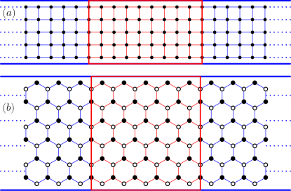
Figure 1: (Color online) A schematic diagram of a infinitely long ribbon on the square lattice for the HgTe/CdTe model (a) and a infinitely long ribbon in the honeycomb lattice along the zigzag direction for the Haldane model (b).

Here $a$ is the lattice constant and all of the parameters $A$, $B$, $C$, $D$, and $M$ can be controlled experimentally5 (5). The topological mass $M$ can be tuned continuously by changing the thickness of the HgTe and subsequently switches the HgTe/CdTe wells between a topologically nontrivial phase and a topologically trivial phase. In this model, the individual spin-up Hamiltonian and spin-down Hamiltonian in Eq. (1) are time-reversal symmetric to each other. Since they are decoupled, we can deal with them individually. For simplicity, we shall focus only on the spin-up Hamiltonian in the following calculations. The Haldane model proposed by Haldane in 1988, Haldane (22) considers honeycomb lattice with next-nearest-neighbor coupling and a staggered sublattice potential. The Hamiltonian can be expressed as: Haldane (22)

$$H_{2} = \sum_{m}{\varepsilon_{m}c^{\dagger}_{m}c_{m}}+\sum_{\langle m,n\rangle}{t_{mn}c^{\dagger}_{m}c_{n}}+t_{2}\sum_{\langle\langle m,n\rangle\rangle}e^{i\upsilon_{mn}\phi}{c^{\dagger}_{m}c_{n}}.$$

The first term is the onsite energy and $\varepsilon_{m}=\pm\Delta$ for the A site (B site), which is shown by a dot (circle) in Fig. 1(b). The second term is the usual nearest neighbor hopping term. Here, random bond disorder is introduced by $t_{mn}=t_{nm}=t_{1}+\delta t_{r}$, where $\delta t_{r}$ is uniformly distributed in the range $[-\frac{U}{2},\frac{U}{2}]$ with the disorder strength $U$. Note that the random hopping term gives the bond disorder a more concrete physical image of the underlying nature of the term. The third term is the second neighbor hopping term with bond dependent phase. Note that $\upsilon_{mn}$ is different for different hopping directions. 1 (1, 22, 11) For example, if an electron in A or B site makes a left (right) turn to get to the second site, $\upsilon_{mn}=1(-1)$. By performing Fourier transformations, we can easily obtain the low energy effective Hamiltonian for the two models given above. Note that the low energy effective Hamiltonian for the two models have the same representation and can be written as follows: 6 (6)

$$H(\hat{k}) = H_{0}(\hat{k})+V=\alpha(\hat{k}_{x}\sigma_{x}-\hat{k}_{y}\sigma_{y})$$ (18)

$$+ (M+\beta\hat{k}^{2})\sigma_{z}+(\mu+\gamma\hat{k}^{2})\sigma_{0}+U(r)\sigma_{d},$$

where the operator $\hat{k}_{x/y}$ can be represented with the momentum operator: $\hat{k}_{x/y}=-i\hbar\partial_{x/y}$. This Hamiltonian is a two-dimensional Dirac Hamiltonian where the three Pauli matrices $\sigma_{x}$, $\sigma_{y}$, $\sigma_{z}$ and the unit matrix $\sigma_{0}$ represent the pseudospins. Note that the pseudospin is formed by the $s$ or $p$ orbital (corresponding to the A or B sublattice) for the HgTe/CdTe (Haldane) model. The scalar potential $U(r)$ accounts for the disorder amplitude and $\sigma_{d}=\sigma_{0/x}$ denotes Anderson disorder or bond disorder respectively. The parameters $\alpha$, $\mu$, $\gamma$ and $\beta$ for the HgTe/CdTe model have the simple form of:

$$\alpha=-A;\hskip 5.69054pt\mu=C;\hskip 5.69054pt\gamma=-D;\hskip 5.69054pt\beta=-B.$$ (19)

Meanwhile, the low energy effective Hamiltonian for the Haldane model can be expanded at the two inequivalent Dirac points $K$ and $K^{*}$. Therefore, the parameters $\alpha$, $\mu$, $M$, $\gamma$ and $\beta$ for the Haldane model can be represented as:

$$\alpha = \frac{3}{2}t_{1}a;\hskip 5.69054pt\mu=-\sqrt{3}t_{2}cos\phi;\hskip 5.69054ptM=\Delta\pm 3\sqrt{3}t_{2}sin\phi,$$

$$\gamma = \frac{9}{4}t_{2}a^{2}cos\phi;\hskip 5.69054pt\beta=\mp\frac{9\sqrt{3}}{4}t_{2}a^{2}sin\phi,$$ (20)

where $\pm$ or $\mp$ corresponds to $K$ or $K^{*}$ respectively. It has been explained Beenakker (13) that elastic scattering by onsite Anderson disorder (called $\sigma_{0}$ disorder to distinguish it from bond disorder being called $\sigma_{x}$ disorder correspondingly in this paper) causes a state with a definite momentum to decay exponentially as a function of space and time. Therefore, a negative correction to the topological mass $M$ is induced due to the quadratic term in the Hamiltonian. The renormalized mass $\overline{M}=M+\delta M$ may, in fact, have the opposite sign to the bare mass $M$. This implies that onsite Anderson disorder, $\sigma_{0}$, may induce a phase transition from a normal insulator to the topological phase. When this happens, TAI phenomena can be observed. However, the question arises as to whether this applies to the bond disorder, namely $\sigma_{x}$ disorder. We will now qualitatively show this mechanism through the following derivation. First, we begin with the Hamiltonian in Eq. (3). Following the same derivation given in the paper by Groth et al., Beenakker (13) the self-energy can be obtained from the equation:

$$[E-H_{0}(k)-\Sigma(E,k)]^{-1} = \langle[E-H(k)]^{-1}\rangle,$$ (21)

where $\langle\ldots\rangle$ denotes the disorder average. Then, the self-energy can be represented in the form: $\Sigma(E,k)=\Sigma_{0}\sigma_{0}+\Sigma_{x}\sigma_{x}+\Sigma_{y}\sigma_{y}+\Sigma_{z}\sigma_{z}$. Obviously, the role of $\Sigma(E,k)$ induced by $\sigma_{0}$ or $\sigma_{x}$ disorder must be to make a correction to the $\sigma_{i}$ terms in $H(k)$. The topological mass and the chemical potential are then renormalized and take the form:

$$\overline{M}=M+\lim_{k\rightarrow 0}Re\Sigma_{z},\ \ \ \ \ \overline{\mu}=E-\lim_{k\rightarrow 0}Re\Sigma_{0}.$$ (22)

To acquire self-energy $\Sigma(E)$ in numerical calculations, the self-consistent Born approximation is applicable and the integral equation for $\Sigma(E)$ and can be written as:

$$\Sigma(E)=\frac{U^{2}}{12}(a/2\pi)^{2}\int_{BZ}d^{2}k[\sigma_{d}(E^{+}I-H_{0}-\Sigma)^{-1}\sigma_{d}],$$ (23)

where $\sigma_{d}=\sigma_{0/x}$ denotes the type of disorder. Up this point, it becomes apparent that the different types of disorder may lead to a different correction to the topological mass, the sign of which is critical for classifying the topological phase of the system. To see this clearly, we neglect $\Sigma(E)$ on the right side of Eq. (8). An approximate solution for $\Sigma(E)$ with a closed form is then given by:

$$\overline{M}=M\mp\frac{U^{2}a^{2}}{48\pi\hbar^{2}}\frac{\beta}{\beta^{2}-\gamma^{2}}ln\mathbf{\bigg{|}}\frac{\beta^{2}-\gamma^{2}}{E^{2}-M^{2}}\mathbf{\bigg{|}}(\frac{\pi\hbar}{a})^{4}$$ (24)

$$\overline{u}=E-\frac{U^{2}a^{2}}{48\pi\hbar^{2}}\frac{\gamma}{\beta^{2}-\gamma^{2}}ln\mathbf{\bigg{|}}\frac{\beta^{2}-\gamma^{2}}{E^{2}-M^{2}}\mathbf{\bigg{|}}(\frac{\pi\hbar}{a})^{4}$$ (25)

where $\mp$ corresponds to $\sigma_{0}$ and $\sigma_{x}$ disorder respectively. For random bond disorder, the $\sigma_{0}$ term in the self-energy $\Sigma(E,k)$ above is obtained by $\sigma_{x}\sigma_{0}\sigma_{x}=\sigma_{0}$; for normal Anderson disorder, it may be calculated using $\sigma_{0}\sigma_{0}\sigma_{0}=\sigma_{0}$. Thus, the $\sigma_{0}$ term does not produce any difference for the two types of disorder, and the Fermi energy, which corresponds to the $\sigma_{0}$ term, has the same renormalization for normal Anderson disorder, $\sigma_{0}$ and bond disorder, $\sigma_{x}$. However, the $\sigma_{z}$ term in the self-energy $\Sigma(E,k)$ is changed differently by Anderson disorder and bond disorder. Because $\sigma_{0}\sigma_{z}\sigma_{0}=\sigma_{z}$ and $\sigma_{x}\sigma_{z}\sigma_{x}=-\sigma_{z}$, the topological mass, which corresponds to the $\sigma_{z}$ term, is renormalized along opposite directions by Anderson disorder $\sigma_{0}$ and bond disorder $\sigma_{x}$. This can be seen clearly in Eq. (9). Hence, TAI phenomenon in a $\sigma_{x}$ disordered system may manifest different features from that in a $\sigma_{0}$ disordered system. Although the above formula are derived in the HgTe/CdTe quantum wells, they should be also applicable to the Haldane model since the low energy effective Hamiltonian for the two models have the same representation as BHZ model. 6 (6) In addition, it should point out that the disorder-induced mass inversion always corresponds to a topological phase transition in HgTe/CdTe quantum wells, however it is not true for the Haldane model if the topological mass only change its sign at K or K^∗ point. That is because the topological property of the Haldane model is determined by the relative sign of the topologically effective mass at the two Dirac points K and K^∗. Namely, if the topological masses have opposite sign at K and K^∗ points, the system is topologically non-trivial. Otherwise, the system is topologically trivial. In the following, we will see clearly that the disorder, regardless of Anderson disorder or bond disorder, has the same effects on the two models. From the models in Eqs. (1) and (2), it is easy to describe a nanoribbon geometry as shown in Fig. 1. Here, only the nanoribbon with a zigzag edge is studied for the Haldane model. Using the Landauer-Büttiker formula, the linear conductance at zero temperature and low bias voltage can be represented as: Jiang (9, 23, 24)

$$G_{LR} = \frac{e^{2}}{h}T=\frac{e^{2}}{h}Tr{[\Gamma_{L}G^{r}\Gamma_{R}G^{a}]},$$ (26)

where $T=Tr{[\Gamma_{L}G^{r}\Gamma_{R}G^{a}]}$ is the transmission coefficient from the left lead (source) to the right lead (drain), $\Gamma_{L/R}=i(\Sigma^{r}_{L/R}-\Sigma^{a}_{L/R})$ with $\Sigma^{r/a}_{L/R}$ being the retarded/advanced self energy, respectively. To present a more concrete picture, we will provide some numerical calculations for the two models and follow with discussions on the implications in section III.

III Numerical Results and Discussions

III.1 Band structures for two models

In this section, the conductance, conductance fluctuations and localization length are studied numerically. The size of the central region is denoted by integers N and W, which represent the length and width respectively. For example, in the schematic diagram shown in Fig. 1(a), the length of the central region (red) is given by $L_{x}=N\times a$ with $N=9$, and the width by $L_{y}=W\times a$ with $W=5$. In Fig. 1(b), the length of the central region (red) is given by $L_{x}=N\times\sqrt{3}a$ with $N=5$, and the width by $L_{y}=W\times\sqrt{3}a$ with $W=3$. Here, $a$ is the square lattice constant $a=5$nm for the HgTe/CdTe model and represents the nearest neighboring distance of $a=0.142$nm for the Haldane model.

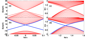
Figure 2: (Color online) The band structures for the HgTe/CdTe and Haldane models are shown in (a), (b) and (c), (d). (a) and (b) are plotted with different topological masses of $M=1$meV and $M=-10$meV; (c) and (d) are plotted with different staggered terms of $\Delta=-1.77t$ and $\Delta=-1.60t$. The red (blue) lines represent the bulk states (edge states).

We have plotted the band structures of the two models in Fig. 2. Figs. 2(a) and 2(b) are plotted for the HgTe/CdTe model with parameters $M=1$meV 2(a) and $M=-10$meV 2(b); Figs. 2(c) and 2(d) are for the Haldane model with $\Delta=-1.6t$ 2(c), and $\Delta=-1.77t$ 2(d). In the numerical calculations, other sample-specific parameters are fixed to be $A=364.5$meV$\cdot$nm, $B=-686$meV$\cdot$nm², $C=0$, $D=-512$meV$\cdot$nm² for the HgTe/CdTe model. For the Haldane model, $t$ is set as the energy unit ($t=1$), and other parameters are set with values of $t_{1}=-t$, $t_{2}=-0.5t$, $\phi=-0.235\pi$. It can be clearly seen that for the topologically nontrivial phase of two models, gapless states traverse the bulk gap in Figs. 2(b) and 2(d). When changing the topological mass from the topologically nontrivial phase to the topologically trivial phase, gapless states disappear from the bulk gap for 2(a) and 2(c). If the stripe geometry in Figs. 1(a) and 1(b) has a periodic boundary in the $y$ direction, namely transforming the system into a cylindrical geometry, the gapless edge states disappear in 2(b) and 2(d), but no visible changes can be observed in 2(a) and 2(c). For simplicity, the band structures for the cylindrical geometry are not shown here. This means that the two systems are both 2D topologically trivial insulators for the parameters in Figs. 2(a) and 2(c) but are topologically nontrivial insulators for the parameters in Figs. 2(b) and 2(d).

III.2 The conductance and its fluctuations

In Figs.(3) and (4), we investigate the conductance and its fluctuations versus strength of the two types of disorder in the models. In all of these calculations data are averaged for 500 random configurations of disorder. Note that for Anderson disorder, the results show the same physics as that described in previous papers Shen (8, 9, 13) for the HgTe/CdTe model [see Figs. 3(a) and 3(c)]. The conductance and its fluctuations are specifically studied for the Haldane model with Anderson disorder [see Figs. 4(a) and 4(c)] and the same quantum conductance plateau and zero conductance fluctuation can be seen within a definite range of Anderson disorder. Thus, for Anderson disorder, we find the following properties: First, the conductance decays and its fluctuations initially increases gradually when increasing strength of Anderson disorder. Second, at moderate Anderson disorder strength, the conductance stops deceasing and falls to a quantum plateau ($e^{2}/h$, when considering only spin up or spin down case). In addition, the conductance fluctuation reduces to zero [see Fig. 3(c)] or a very small value [see Fig. 4(c)] over the corresponding range of Anderson disorder strength. Note25 (25) Third, as the strength of Anderson disorder continues to increase, the conductance and its fluctuations both decrease gradually to zero. The system thus finally transforms to an Anderson insulator when the disorder is sufficiently strong.

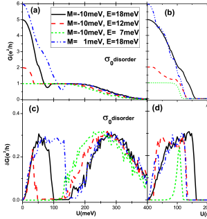
Figure 3: (Color online) The conductance $G$ (a), (b) and conductance fluctuations $\delta G$ (c), (d) vs disorder strength U for the HgTe/CdTe model. Different curves correspond different Fermi energy $E$ or different topological masses. The size of the central region is set at $L_{x}=200a$, $L_{y}=80a$. Other parameters (A, B, C and D) are given at the beginning of Sec. III. Here, $\sigma_{0}$ and $\sigma_{x}$ disorders correspond to Anderson disorder and bond disorder respectively.

In general, the quantum conductance plateau and zero conductance fluctuations always imply a new phase or a novel phenomenon. From the results about the quantum conductance, TAI was initially found three years ago. Shen (8) As mentioned in Introduction, Groth et al. Beenakker (13) showed how Anderson disorder induce a phase transition. Namely, Anderson disorder will add a negative correction to the topological mass. When the topological mass changes its sign at strong Anderson disorder strength, a phase transition is triggered from the topologically trivial phase to the topologically nontrivial phase. However, due to the extensive existence of bond disorder in real materials, it is necessary and important to study what happens when considering bond disorder. In Figs. 3(b), 3(d), 4(b), and 4(d), the conductance and its fluctuations are investigated for the two models with bond disorder. Contrary to the case of Anderson disorder, TAI is not observed in the two models when changing the strength of bond disorder. For example, for the HgTe/CdTe model in Figs. 3(b) and 3(d), a series of topological masses $M$ and Fermi energies $E$ are chosen. In each case, the conductance gradually falls to zero and the quantum plateau shown in Fig. 3(a) disappears completely. Moreover, the conductance fluctuations in Fig. 3(d) only shows a peak and then falls to zero finally because of the Anderson localization. This description is also qualitatively true for the Haldane model in Figs. 4(b) and 4(d). Therefore, it can be concluded that bond disorder cannot induce a phase transition to TAI for the two models as discussed above in Sec. II.

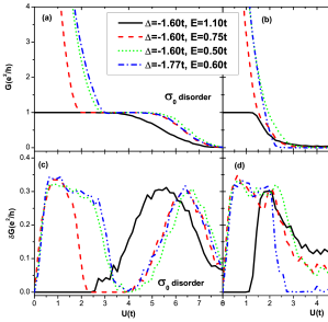
Figure 4: (Color online) The conductance $G$ (a), (b) and conductance fluctuations $\delta G$ (c), (d) vs disorder strength U for Haldane model. Different curves correspond to different Fermi energies $E$ or staggered terms $\Delta$. The size of the central region is set to be $L_{x}=200\times\sqrt{3}a$, $L_{y}=92\times 3a$. Other parameters ($t_{1}$, $t_{2}$, and $\phi$) are given at the beginning of Sec. III. Here, $\sigma_{0}$ and $\sigma_{x}$ correspond to Anderson disorder and bond disorder respectively.

III.3 The conductance phase diagrams for two types of disorder

To see this more clearly, the conductance phase diagrams are compared for Anderson disorder and bond disorder in the HgTe/CdTe model. The results, in Figs. 5(a), 5(c), 6(a), and 6(c), are shown for normal Anderson disorder; Figs. 5(b), 5(d), 6(b), and 6(d) correspond to bond disorder. It can be seen from Figs. 6(a), and 6(c) that at moderate Anderson disorder and Fermi energy, a clear TAI phase (green region) is present and that the TAI phase in Fig. 6(c) must correspond to a negative renormalized topological mass $\overline{M}$ (blue region). The Anderson disorder renormalizes the topological mass $M$ along the negative direction and Fermi energy along the positive direction and therefore induced a phase transition to TAI. The results in Figs. 5(a), 5(c), 6(a), and 6(c) are similar to those described in previous papers. Shen (8, 9, 13) In summary, normal Anderson disorder can localize the bulk states. For a original system of a topological nontrivial phase [Fig. 5(a)], the edge state is more robust against Anderson disorder than are bulk states and thus leads to a quantum conductance region (green region). For a original system with a topologically trivial phase [Fig. 6(a)], a phase transition from a topologically trivial insulator to a topological insulator can occur as the strength of Anderson disorder increases, and thus result in a TAI quantum conductance region (green region). For Anderson disorder, the topological mass is always renormalized by adding a negative correction. A more detailed interpretation can be found in several previous papers. Shen (8, 9, 13)

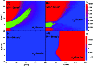
Figure 5: (Color online) The conductance $G$ (a), (b) and topological mass $\overline{M}$ (c), (d) vs disorder strength U for the HgTe/CdTe model with $M=-10$meV. The size of the central region is set to be $L_{x}=200a$, $L_{y}=80a$. Other parameters (A, B, C, and D) are given at the beginning of Sec. III. Here, $\sigma_{0}$ and $\sigma_{x}$ correspond to Anderson disorder and bond disorder respectively.

In the following, we are more concerned about the influence of bond disorder on this phenomenon. It can be seen from Fig. 5 that at $M=-10$meV, the quantum conductance region with a value of $e^{2}/h$ (green region) above the band gap in Fig. 5(a) disappears completely as shown in Fig. 5(b). Namely, the quantum conductance region where the value of the conductance is $e^{2}/h$ (green region) decays to a very small region, and only exists within the band gap and at a small strength of bond disorder [Fig. 5(b)]. The renormalized mass $\overline{M}$, which remains negative for the whole phase diagram of Fig. 5(c) (blue region), alters its sign between the range of $100$ meV $\lesssim U\lesssim 150$meV in Fig. 5(d). Thus, there are very different effects on the mass $M$ for the two types of disorder. It may be surprising that a larger phase region of bulk states (red region) appears in Fig. 5(b) than in Fig. 5(a). This implies a greater difficulty in localizing the bulk states for the case of bond disorder compared to the case of Anderson disorder. This result is understandable if the different effects of Anderson disorder and bond disorder are considered. Anderson disorder renormalizes the topological mass $M$ along positive direction. That is, the effective band gap became larger and thus bulk states are shifted upward for the Anderson disorder case. On the contrary, the opposite effect appeared for the bond disorder. Because states in the center of the bulk band are more difficult to localize than states near the edge of bulk band, Thouless (29) a larger phase region of bulk states is observed in Fig. 5(b) for bond disorder than that in Fig. 5(a) for Anderson disorder. Note that the conclusions above are based on the same renormalization of the chemical potential $\overline{\mu}$ for both disorder types as given in Eq. (10).

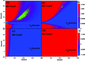
Figure 6: (Color online) The conductance $G$, (a), (b) and renormalized topological mass $\overline{M}$ (c), (d) vs disorder strength U and Fermi level $E$ for the HgTe/CdTe model with $M=1$meV. The size of the central region is set to be $L_{x}=200a$, $L_{y}=80a$. Other parameters (A, B, C, and D) are given at the beginning of Sec. III. Here, $\sigma_{0}$ and $\sigma_{x}$ correspond to the Anderson disorder and bond disorder respectively.

When the system turns to a topologically trivial phase with $M=1$meV as in Fig. 6, there is no indication of the TAI phenomenon in the conductance phase diagram, Fig. 6(b). That is, the conductance region with the value of $e^{2}/h$ disappears completely for bond disorder. Meanwhile, in the phase diagram with a topological mass $M=1$meV as shown in Fig. 6(d), the topological phase (blue region) gives way to the topologically trivial phase (red region) and the whole diagram is governed by positive renormalized topological mass (red region). Therefore, a clear conclusion can be drawn from these numerical results that normal Anderson disorder gives rise to the TAI phenomenon and bond disorder destroys it. In other words, whether the TAI phenomenon can be observed depends on a competition between Anderson disorder and bond disorder in a system because Anderson disorder and bond disorder renormalize the topological mass along different directions and thus affect TAI phenomena differently.

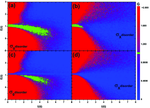
Figure 7: (Color online) The conductance $G$ vs. disorder strength U and Fermi level $E$ for the Haldane model. (a) and (b) are plotted with $\Delta=-1.6t$ in a topologically nontrivial region; (c) and (d) with $\Delta=-1.77t$ in a topologically trivial region. The size of the central region is set to be $L_{x}=200\times\sqrt{3}a$, $L_{y}=92\times 3a$. Other parameters are chosen with $\phi=-0.235\pi$, $t_{2}=-0.5t$. Here, $\sigma_{0}$ and $\sigma_{x}$ correspond to the Anderson disorder and bond disorder respectively.

The above conclusions are also applicable to the Haldane model. When considering Anderson disorder in Fig. 7(a) with the topologically nontrivial phase and 7(c) with the topologically trivial phase, the conductance phase diagrams show a clear region with quantize conductance $G_{0}$ (green region), which is the hallmark of TAI in Fig. 7(c). However, for bond disorder, the region of quantized conductance becomes indistinguishable in Fig. 7(b) for the topologically nontrivial phase and in 7(d) for the topologically trivial phase. This indicates that Anderson disorder can drive a phase transition to TAI but that bond disorder can not. Here, we do not give a topological mass diagram similar to Fig. 5(c) or 5(d) for the HgTe/CdTe model because the Haldane model is based on the honeycomb lattice which means that the topological properties of this model are determined by the signs of the effective masses at the two Dirac points, as introduced in Sec. II. When the signs of the effective masses at two Dirac points are opposite, the band at one Dirac point would be inverted from that at another Dirac point, and the system is topologically non-trivial. Conversely, when the sign of the effective mass at two Dirac points is the same, the system corresponds to a topologically trivial phase. In addition, the parameter $\beta$ in Eq. (5) has different expressions at the two the Dirac points. Consequently, it is difficult to present clearly the variation of the topological properties as a function of the disorder strength using a simple phase diagram of the topological mass.

III.4 The localization lengths for two types of disorder

In order to highlight the dependence of TAI on the type of disorder, we also plot the localization length Beenakker (13, 26, 27, 28) $\lambda/L_{y}$ of a 2D ribbon with width $L_{y}=W\times a$ for the square lattice [Figs. 8(a) and 8(c)] and $L_{y}=W\times 3a$ for the honeycomb lattice [Figs. 8(b) and 8(d)]. Note that the localization length is obtained from the relationship Beenakker (13) $\lambda\equiv 2$lim${}_{L_{x}\rightarrow\infty}L_{x}\langle$ln$(G/G_{0})\rangle^{-1}$ by increasing the length $L_{x}$ of the system at fixed width $L_{y}$, namely, $L_{x}\gg L_{y}$. In addition, another calculating method, transfer-matrix method, MacKinnon (26, 27, 28) is also adopted to guarantee the correctness of the localization length. Here we have considered both cylindrical geometry and ribbon geometry. For the HgTe/CdTe model, the localization length $\lambda/L_{y}$ shown in in Fig. 8(a) first deceases when increasing disorder strength for Anderson disorder. With further increasing the strength of Anderson disorder, a peak appears for the localization length $\lambda/L_{y}$ and then decays gradually for both geometries, which can be seen clearly in Fig. 8(a). The difference in localization length $\lambda/L_{y}$ between the two geometries is that peaks have distinct heights and are located at the different strengths of Anderson disorder. It can be deduced that because of existing edge states, a special metal phase emerges for the ribbon geometry near to the position of the peak. However, when considering bond disorder, the peak of the localization length $\lambda/L_{y}$ vanishes completely as shown in Fig. 8(c). This provide a further evidence that bond disorder does not induce a phase transition to TAI. As is shown in Fig. 8(b) and 8(d) for the Haldane model, there is no essential difference with the results shown in Figs. 8(a) and 8(c) for the HgTe model.

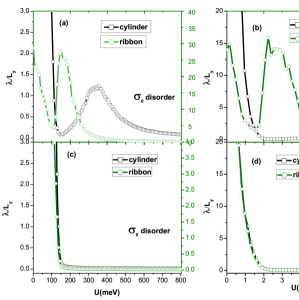
Figure 8: (Color online) Localization length vs disorder strength U for the HgTe/CdTe model (a), (c) and for the Haldane model (b), (d). (a), (b) and (c), (d) correspond to $\sigma_{0}$ and $\sigma_{x}$ disorder respectively. In the calculations, the Fermi energy $E$ is set to be $E=25$meV, the topological mass is $M=-10$meV and the width of the ribbon is $L_{y}=50a$ for the HgTe/CdTe model. The Fermi energy is $E=0.80t$, the staggered term is $\Delta=-1.60t$ and the width of the ribbon is $L_{y}=40\times 3a$ for the Haldane model. The black line and green line are plotted for the ribbon and cylindrical geometry respectively. Here, $\sigma_{0}$ and $\sigma_{x}$ correspond to the Anderson disorder and bond disorder respectively.

IV Conclusions

In summary, we have studied the influence of bond disorder (called $\sigma_{x}$ disorder) on two models. This type of disorder can originate in the deformation of the lattice, mismatch between two lattices or some chemical effects and thus exists extensively in many real materials. Unlike normal Anderson disorder, bond disorder does not induce a phase transition to a topological Anderson insulator(TAI). This is analytically verified by using Born approximation theory. The conductance and its fluctuations are then calculated, and the conductance plateau, which is the hallmark of TAI, is very good for Anderson disorder but becomes barely distinguishable for bond disorder. In addition, phase diagrams are compared for two models with two types of disorder, Anderson disorder $\sigma_{0}$ and bond disorder $\sigma_{x}$. For Anderson disorder, the TAI phase can be seen clearly in the phase diagrams. However, the TAI phase disappears for bond disorder. Because of a effective characterization in the metal-insulator phase transition, the localization length of the wave function is studied for the two models with Anderson and bond disorders. For the two models with normal Anderson disorder, the localization length shows a peak at moderate disorder region, which exactly corresponds to TAI phase. However, the wave functions are localized quickly and no peak of localization length can be seen for the system with bond disorder. That means that Anderson disorder and bond disorder can play different roles in the topological phase transition. To sum up, bond disorder can prohibit the system undergoing a phase transition to TAI, contrary to what may be seen in a Anderson disordered insulator. Note30 (30) These general conclusions in this paper are not restricted to two-dimensional systems and further work in a three-dimensional systems, e.g. $Bi_{2}Se_{3}$ model, 4 (4) will be needed. If researchers intend to change the property of a topological insulator by addition of impurities, eg. shifting the energy level from the bulk states to the bulk gap, it will be necessary to guarantee that the impurities are mainly of the Anderson disorder type but keeps away from the bond disorder type. This is a key point for the doping process in preparation of topological insulators.

References

- (1) Electronic address: jianghuaphy@gmail.com
- (2) C. L. Kane and E. J. Mele, Phys. Rev. Lett. 95 226801 2005; 95, 146802 (2005).
- (3) C. Day, Phys. Today, 61 (1), 19 (2008); N. Nagaosa, Science 318, 758 (2007).
- (4) D. Hsieh, D. Qian, L. Wray, Y. Xia, Y. S. Hor, R. J. Cava, and M. Z. Hasan, Nature (London) 452, 970 (2008); L. Fu, C. L. Kane, and E. J. Mele, Phys. Rev. Lett. 98, 106803 (2007).
- (5) H. Zhang, C. Liu, X. Qi, X. Dai, Z. Fang, and S. C. Zhang, Nat. Phys. 5, 438 (2009).
- (6) M. Knig, S. Wiedmann, C. Brne, A. Roth, Hartmut Buhmann, Laurens W. Molenkamp, X.-L. Qi and S.-C. Zhang, Science 318, 766 (2007); M. Knig, H. Buhmann, L. W. Molenkamp, T. L. Hughes, C.-X. Liu, X.-L. Qi, and S.-C. Zhang, J. Phys. Soc. Jpn. 77, 031007 (2008).
- (7) B. A. Bernevig, T. L. Hughes, and S. C. Zhang, Science 314, 1757 (2006).
- (8) H. Jiang, S. G. Cheng, Q.-F. Sun, and X. C. Xie, Phys. Rev. Lett. 103, 036803 (2009).
- (9) J. Li, R. L. Chu, J. K. Jain, and S. Q. Shen, Phys. Rev. Lett. 102, 136806 (2009).
- (10) H. Jiang, L. Wang, Q.-F. Sun, and X. C Xie, Phys. Rev. B, 80, 165316 (2009).
- (11) H.-M. Guo, G. Rosenberg, G. Refael, and M. Franz, Phys. Rev. Lett. 105, 216601 (2010).
- (12) Y. Xing, L. Zhang, and J. Wang, Phys. Rev. B 84, 035110 (2011).
- (13) A. Yamakage, K. Nomura, K. Imura, and Y. Kuramoto, J. Phys. Soc. Jap., 80, 053703 (2011).
- (14) C. W. Groth, M. Wimmer, A. R. Akhmerov, J. Tworzydło, and C. W. J. Beenakker, Phys. Rev. Lett. 103, 196805 (2009).
- (15) E. Prodan, Phys. Rev. B 83, 195119 (2011).
- (16) L. Chen, Q. Liu, X. Lin, X. Zhang, X. Jiang and T.-H. Lin, arXiv:1106.4103.
- (17) Y.Y. Zhang, R.L. Chu, F.C. Zhang, and S.Q. Shen, Phys. Rev. B 85, 035107 (2012).
- (18) X. Jia, P. Goswami, and S. Chakravarty, Phys. Rev. Lett. 101, 036805 (2008); J. C. Woicik, J. G. Pellegrino, B. Steiner, K. E. Miyano, S. G. Bompadre, L. B. Sorensen, T.-L. Lee, and S. Khalid, Phys. Rev. Lett. 79, 5026 (1997); H. Shinaoka, Y. Tomita, and Y. Motome, Phys. Rev. Lett. 107, 047204 (2011).
- (19) A. Altland, Phys. Rev. B 65, 104525 (2002); P. M. Ostrovsky, I. V. Gornyi, and A. D. Mirlin, Phys. Rev. B 74, 235443 (2006); E. McCann, K. Kechedzhi, V. I. Fal′ko, H. Suzuura, T. Ando, and B. L. Altshuler, Phys. Rev. Lett. 97, 146805 (2006).
- (20) P. M. Ostrovsky, I. V. Gornyi, and A. D. Mirlin, Phys. Rev. Lett. 98, 256801 (2007); F. Evers, A. D. Mirlin, Rev. Mod. Phys. 80, 1355 (2008).
- (21) K. Nomura and N. Nagaosa, Phys. Rev. Lett. 106, 166802 (2011); S. A. Yang, Z. Qiao, Y. Yao, J. Shi, and Q. Niu, Europhys. Lett. 95, 67001 (2011).
- (22) Note that in HgTe/CdTe quantum wells only the same-cell bond disorder are studied and the bond disorder, wich represents a random correction the different-orbital hopping terms in the same cell. When considering the different-cell disorders, the same orbital hopping disorder, which means a random correction to the hopping terms between the same orbital, i.e. and in this paper, will play a similar role as Anderson disorder in the same cell, while the different-orbital hopping disorder, which means a random correction to the hopping term between the different orbital, i.e. in this paper, will play a similar role as bond disorder in the same cell.
- (23) F. D. M. Haldane, Phys. Rev. Lett. 61, 2015 (1988).
- (24) T. P. Pareek, Phys. Rev. Lett. 92, 076601 (2004); Juntao Song, Q.-F. Sun, Jinhua Gao, and X. C. Xie, Phys. Rev. B 75, 195320 (2007); Y. Xing, Q.-F. Sun, and J. Wang, Phys. Rev. B 73, 205339 (2006); Phys. Rev. B 80, 235411 (2009).
- (25) Electronic Transport in Mesoscopic Systems, edited by S. Datta (Cambridge University Press 1995).
- (26) The size effect of TAI has been studied numerically in the Haldane model. It is found that whether the quantum conductance plateau and zeros conductance fluctuation exist is independent of the size of the system. Thus, in the Haldane model, the TAI phenomena should be a robust phase not a size fluctuation effect.
- (27) A. MacKinnon and B. Kramer, Phys. Rev. Lett. 47, 1546 (1981); Z. Phys. B 53, 1 (1983).
- (28) B. Kramer and A. MacKinnon, Rep. Prog. Phys. 56, 1469 (1993).
- (29) J.-L. Pichard and G. Sarma, J. Phys. C: Solid State Phys. 14 L127 (1981); 14 L617 (1981).
- (30) D. J. Thouless, Phys. Rep. 13, 93 (1974).
- (31) Note that when bond and Anderson disorder exist simultaneously, the renormalized mass term depends on competition between bond disorder and Anderson disorder. To give an example, a TAI phase can be observed when Anderson disorder strength is much stronger than bond disoder. On the contrary, the TAI phase does not show up when bond disorder is stronger than Anderson disorder. Thus, whether TAI can be observed in this case just depends on which type of the two disorders is stronger.