Theoretical calculations on the structural, electronic and optical properties of bulk silver nitrides

Abstract

We present a first-principles investigation of structural, electronic and optical properties of bulk crystalline Ag₃N, AgN and AgN₂ based on density functional theory (DFT) and many-body perturbation theory. The equation of state (EOS), energy-optimized geometries, cohesive and formation energies, and bulk modulus and its pressure derivative of these three stoichiometries in a set of twenty different structures have been studied. Band diagrams and total and orbital-resolved density of states (DOS) of the most stable phases have been carefully examined. Within the random-phase approximation (RPA) to the dielectric tensor, the single-particle spectra of the quasi electrons and quasi holes were obtained via the GW approximation to the self-energy operator, and optical spectra were calculated. The results obtained were compared with experiment and with previously performed calculations.

I Introduction

It is well-known now that late transition-metal nitrides (TMNs) usually possess interesting properties leading to a variety of potential technological applications PhysRevB.82.104116 ; OsCarbides_2010 ; MorenoArmenta2007166 . Hence, a significant number of quantum mechanical ab initio calculations of the structural and physical properties of this family of materials have appeared in the literature.

Since Juza and Hahn the_first_Cu3N_1939_exp succeeded to synthesize Cu₃N in 1939, copper nitrides have been produced through various techniques and their properties and applications have been the subject of many theoretical and experimental published works Suleiman_PhD_arXiv2012_copper_nitrides_article . Due to its early discovery, copper nitride may now be considered as the most investigated among the late TMNs nano_Cu3N_2005_exp .

On the other hand, the nitride of silver, the next element to copper in group 11 of the periodic table, has been known for more than two centuries Ag3N_1991_exp ; Ag_Pd_Au_nitrides_PhD_thesis_2010_exp . However, despite its earlier discovery, silver nitride may be the least theoretically studied solid in the late TMNs family. Experimental efforts to investigate structural German_Ag3N_structure_1949_exp ; Ag_Pd_Au_nitrides_PhD_thesis_2010_exp , electronic Ag_Pd_Au_nitrides_PhD_thesis_2010_exp and formation Ag3N_1991_exp ; Anderson_n_Parlee_1970_exp ; German_Ag3N_structure_1949_exp ; Juza_n_Hahn_1940 properties of silver nitrides have been made by some researchers.

In 1949, Hahn and Gilbert German_Ag3N_structure_1949_exp carried out the first Ag_Pd_Au_nitrides_PhD_thesis_2010_exp structural study on the reported stoichiometry, Ag₃N. They claimed an fcc structure with $a=4.369\;\text{\AA}$ and $Z=4/3$ (i.e. $4$ Ag atoms in the unit cell). A long time later in 1982, Haisa Ag3N_structure_theory_1982 suggested that the Ag atoms are located at the corners and face centers of the unit cell, while the N atoms, which may be statistically distributed in the octahedral interstices, were given no definite positions Ag3N_structure_theory_1982 .

According to the calculated N radius, Ag₃N can be described as an ionic compound, and recent ab initio calculations on the proposed structure revealed insulating characteristics with a fundamental band gap close to $1.35\;eV$. On the other hand, due to the similar lattice of the parent Ag and the easily separated N as N₂, it can also be argued that this compound is a metal, supporting its black color Ag_Pd_Au_nitrides_PhD_thesis_2010_exp .

Under ordinary conditions Ag3N_1991_exp , it was found that silver can form Ag₃N from ammoniacal solutions of silver oxide Ag3N_1991_exp ; Ag_Pd_Au_nitrides_PhD_thesis_2010_exp . The black metallic-looking solid outcome, Ag₃N, is an extremely sensitive explosive compound Ag3N_1991_exp ; Hazardous_Silver_Compounds_1991 . It may explode due to the slightest touch, even from the impact of a falling water droplet Hazardous_Silver_Compounds_1991 , but it is relatively easy to handle under water or ethanol Ag_Pd_Au_nitrides_PhD_thesis_2010_exp . The explosive power is due to the energy released during the decomposition reaction:

$$2\text{Ag}_{3}\text{N}\longrightarrow 6\text{Ag}+\text{N}_{2}\;.$$ (2)

Even in storage at room temperature, this solid compound decomposes slowly according to Eq. 2 above Hazardous_Silver_Compounds_1991 ; Ag_Pd_Au_nitrides_PhD_thesis_2010_exp . From a thermochemical point of view, it was found that there is no stable intermediate stage in this decomposition, but there may be a metastable intermediate species (phase) with a remarkably low decomposition rate Ag3N_1991_exp . At this point, it may be worth mentioning that the thermochemistry of silver nitride systems is not fully documented in standard handbook data Ag3N_1991_exp .

In their 1991 work, Shanley and Ennis Ag3N_1991_exp stated: “Many of the samples … did not survive the minimum handling required to move them, container and all, to the X-ray stage. … More vigorously explosive samples propagated throughout their mass leaving no visible residue. Even among supersensitive materials, silver nitride is a striking example of a compound “teetering on the edge of existence”. Under the circumstances, we did not succeed in developing data on the proportion of silver nitride required for explosive behavior in these mixtures.”

Thus, beside the potential hazard to lab workers due to its sensitive explosive behavior, characterization of silver nitride is hindered by its extremely unstable (endothermic) nature Ag3N_1991_exp ; Ag_Pd_Au_nitrides_PhD_thesis_2010_exp , and we are presented with an incomplete picture of structural, electronic and optical properties of this material. Surprisingly, this lack of detailed knowledge of many physical properties of silver nitride stimulated only very few published ab initio studies.

In the present work, first-principles calculations were carried out to investigate the lattice parameters, equation of state, relative stabilities, phase transitions, electronic and optical properties of silver nitrides in three different chemical formulae and in various crystal structures. Calculation methods are described in Sec. II. In Sec. III, results are presented, discussed and compared with experiment and with previous calculations. The article is concluded with some remarks in Sec. IV.

II Calculation Methods

II.1 Stoichiometries and Crystal Structures

To the best of our knowledge, the only experimentally reported stoichiometries of Ag-N compounds are Ag₃N Ag3N_1991_exp and AgN₃ Ag3N_1991_exp . However, previous ab initio studies on Ag-N compounds considered Ag₄N Ag_Pd_Au_nitrides_PhD_thesis_2010_exp , Ag₃N AgN_AgN2_Ag2N_Ag3N_2010_comp ; Ag_Pd_Au_nitrides_PhD_thesis_2010_exp , Ag₂N AgN_AgN2_Ag2N_Ag3N_2010_comp , AgN AgN_AgN2_Ag2N_Ag3N_2010_comp ; CuN_AgN_AuN_2007_comp and AgN₂ AgN2_AuN2_PtN2_2005_comp ; AgN_AgN2_Ag2N_Ag3N_2010_comp in some cubic structures only. Consideration of stoichiometries other than the reported ones is probably due to the fact that many transition metals nitrides (TMs) are known to form more than one nitride StructuralInChem . Hence, our interest in investigating AgN and AgN₂ is based on this fact.

For Ag₃N, we consider the following seven structures: the face-centered cubic structure of AlFe₃ (D0₃), the simple cubic structure of Cr₃Si (A15), the simple cubic structure of the anti-ReO₃ (D0₉), the simple cubic structure of Ag₃Au (L1₂), the body-centered cubic structure of CoAs₃ (D0₂), the hexagonal structure of $\epsilon$-Fe₃N, and the trigonal (rhombohedric) structure of RhF₃.

For AgN, the following four structures were considered: the face-centered cubic structure of NaCl (B1), the simple cubic structure of CsCl (B2), the face-centered cubic structure of ZnS zincblende (B3), the hexagonal structure of NiAs (B8₁), the hexagonal structure of BN (B${}_{\text{k}}$), the hexagonal structure of WC (B${}_{\text{h}}$), the hexagonal structure of ZnS wurtzite (B4), the simple tetragonal structure of PtS cooperite (B17), and the face-centered orthorhombic structure of TlF (B24).

AgN₂ was studied in the following nine structures: the face-centered cubic structure of CaF₂ fluorite (C1), the simple cubic structure of FeS₂ pyrite (C2), the simple orthorhombic structure of FeS₂ marcasite (C18) and the simple monoclinc structure of CoSb₂ (CoSb₂).

II.2 Electronic Relaxation Details

In this work, electronic structure spin density functional theory (SDFT) SDFT_1972 ; SDFT_Pant_1972 calculations as implemented in the VASP codeVasp_ref_PhysRevB.47.558_1993 ; Vasp_ref_PhysRevB.49.14251_1994 ; Vasp_cite_Kressw_1996 ; Vasp_PWs_Kresse_1996 ; DFT_VASP_Hafner_2008 ; PAW_Kresse_n_Joubert have been employed. To self-consistently solve the Kohn-Sham (KS) equations KS_1965

$$\begin{split}\Bigg{\{}-\frac{\hbar^{2}}{2m_{e}}\nabla^{2}+\int d\mathbf{r}^{\prime}\frac{n(\mathbf{r}^{\prime})}{|\mathbf{r}-\mathbf{r}^{\prime}|}+V_{ext}(\mathbf{r})\\ +V_{XC}^{\sigma,\mathbf{k}}[n(\mathbf{r})]\Bigg{\}}\psi_{i}^{\sigma,\mathbf{k}}(\mathbf{r})=\epsilon_{i}^{\sigma,\mathbf{k}}\psi_{i}^{\sigma,\mathbf{k}}(\mathbf{r}),\end{split}$$ (3)

where $i$, $\mathbf{k}$ and $\sigma$ are the band, $\mathbf{k}$-point and spin indices, receptively, VASP expands the pseudo part of the KS one-particle spin orbitals $\psi_{i}^{\sigma,\mathbf{k}}(\mathbf{r})$ on a basis set of plane-waves (PWs). Only those PWs with cut-off energy $E_{cut}\leq 600\;eV$ have been included. The Brillouin zones were sampled using $\mathbf{\Gamma}$-centered Monkhorst-Pack MP_k_mesh_1976 $17\times 17\times 17$ meshes. Any increase in the $E_{cut}$ value or in the density of the $\mathbf{k}$-mesh produces a change in the total energy less than $3\;\text{m}eV/\text{atom}$. For static calculations, partial occupancies were set using the tetrahedron method with Blöchl corrections tetrahedron_method_theory_1971 ; tetrahedron_method_theory_1972 ; ISMEAR5_1994 , while the smearing method of Methfessel-Paxton (MP) MP_smearing_1989 was used in the ionic relaxation, and Fermi surface of the metallic phases has been carefully treated. The Perdew-Burke-Ernzerhof (PBE) parametrization PBE_GGA_1996 ; PBE_GGA_Erratum_1997 ; XC_PBE_1999 of the generalized gradient approximation (GGA) XC_GGA_1988 ; XC_GGA_applications_1992 ; XC_GGA_applications_1992_ERRATUM was employed for the exchange-correlation potentials $V_{XC}^{\sigma,\mathbf{k}}[n(\mathbf{r})]$. The implemented projector augmented wave (PAW) methodPAW_Blochl ; PAW_Kresse_n_Joubert was used to describe the core-valence interactions $V_{ext}(\mathbf{r})$, where the $4d^{10}5s^{1}$ electrons of Ag and the $2s^{2}2p^{3}$ electrons of N are treated explicitly as valence electrons. While for these valence electrons only scalar kinematic relativistic effects are incorporated, the PAW potential treats the core electrons in a fully relativistic fashionDFT_VASP_Hafner_2008 . No spin-orbit interaction of the valence electrons has been considered.

II.3 Geometry Relaxation and EOS

At a set of externally imposed lattice constants, ions with free internal parameters were relaxed until all force components on each ion were less than $0.01\;eV/\text{\AA}$. This is done following the implemented conjugate-gradient (CG) algorithm. After each ion relaxation step, static total energy calculation with the tetrahedron method was performed, and the cohesive energy per atom $E_{coh}$ was calculated from

$$E_{coh}^{\text{Ag}_{m}\text{N}_{n}}=\frac{E_{\text{solid}}^{\text{Ag}_{m}\text{N}_{n}}-Z\times\left(mE_{\text{atom}}^{\text{Ag}}+nE_{\text{atom}}^{\text{N}}\right)}{Z\times(m+n)},$$ (4)

where $Z$ is the number of Ag_mN_n formulas per unit cell, $E_{\text{atom}}^{\text{Ag}}$ and $E_{\text{atom}}^{\text{N}}$ are the energies of the isolated non-spherical spin-polarized atoms, and $m,n=1,2\text{ or }3$ are the stoichiometric weights. The obtained $E_{coh}$ as a function of volume $V$ per atom were then fitted to a Birch-Murnaghan 3rd-order equation of state (EOS)BM_3rd_eos and the equilibrium volume $V_{0}$, the equilibrium cohesive energy $E_{0}$, the equilibrium bulk modulus

$$B_{0}=-V\frac{\partial P}{\partial V}\Big{|}_{V=V_{0}}=-V\frac{\partial^{2}E}{\partial V^{2}}\Big{|}_{V=V_{0}}$$ (5)

and its pressure derivative

$$B^{\prime}_{0}=\frac{\partial B}{\partial P}\Big{|}_{P=0}=\frac{1}{B_{0}}\left(V\frac{\partial}{\partial V}(V\frac{\partial^{2}E}{\partial V^{2}})\right)\Big{|}_{V=V_{0}}$$ (6)

were determined.

II.4 Formation Energy

Beside the cohesive energy, another measure of relative stability is the formation energy $E_{f}$. Assuming that silver nitrides Ag_mN_n result from the interaction between the N₂ gas and the solid Ag(A1) via the reaction (compare with Eq. 2)

$$m\text{Ag}^{\text{solid}}+\frac{n}{2}\text{N}_{2}^{\text{gas}}\rightleftharpoons\text{Ag}_{m}\text{N}_{n}^{\text{solid}},$$ (7)

$E_{f}$ can be given by

$$E_{f}(\text{Ag}_{m}\text{N}_{n}^{\text{solid}})=E_{\text{coh}}(\text{Ag}_{m}\text{N}_{n}^{\text{solid}})\quad\quad\quad\quad\quad\quad$$

$$-\frac{mE_{\text{coh}}(\text{Ag}^{\text{solid}})+\frac{n}{2}E_{\text{coh}}(\text{N}_{2}^{\text{gas}})}{m+n} \;.$$ (8)

Here $m,n=1,2,3$ are the stoichiometric weights and $E_{\text{coh}}(\text{Ag}_{m}\text{N}_{n}^{\text{solid}})$ is the cohesive energy per atom as in Eq. 4. The cohesive energy $E_{\text{coh}}(\text{Ag}^{\text{solid}})$ and other equilibrium properties of the elemental metallic silver are given in Table 1. The cohesive energy of the diatomic nitrogen ($E_{\text{coh}}(\text{N}_{2}^{\text{gas}})$) was found to be $-5.196\;eV/\text{atom}$ corresponding to an equilibrium N–N bond length of $1.113\;\text{\AA}$ (For more details, see Ref. Suleiman_PhD_arXiv2012_copper_nitrides_article, ).

II.5 GWA Calculations and Optical Properties

Although a qualitative agreement between DFT-calculated optical properties and experiment is possible, accurate quantitative description requires treatments beyond the level of DFT PAW_optics . Another approach provided by many-body perturbation theory (MBPT) leads to a system of quasi-particle (QP) equations, which can be written for a periodic crystal as GWA_and_QP_review_1999 ; Kohanoff ; JudithThesis2008

$$\begin{split}\Bigg{\{}-\frac{\hbar^{2}}{2m}\nabla^{2}+\int d\mathbf{r}^{\prime}\frac{n(\mathbf{r}^{\prime})}{|\mathbf{r}-\mathbf{r}^{\prime}|}+V_{ext}(\mathbf{r})\Bigg{\}}\psi_{i,\mathbf{k}}^{QP}(\mathbf{r})\\ +\int d\mathbf{r}^{\prime}\Sigma(\mathbf{r},\mathbf{r}^{\prime};\epsilon_{i,\mathbf{k}}^{QP})\psi_{i,\mathbf{k}}^{QP}(\mathbf{r}^{\prime})=\epsilon_{i,\mathbf{k}}^{QP}\psi_{i,\mathbf{k}}^{QP}(\mathbf{r}).\end{split}$$ (9)

Practically, the wave functions $\psi_{i,\mathbf{k}}^{QP}(\mathbf{r})$ are taken from the DFT calculations. However, in consideration of computational cost, we used a less dense mesh of $\mathbf{k}$-points ($10\times 10\times 10$). The term $\Sigma(\mathbf{r},\mathbf{r}^{\prime};\epsilon_{i,\mathbf{k}}^{QP})$ is the self-energy which contains all the exchange and correlation effects, static and dynamic, including those neglected in our DFT-GGA reference system. In the so-called $GW$ approximation Hedin_1st_GWA_1965 , $\Sigma$ is given in terms of the Green’s function $G$ as

$$\begin{split}\Sigma_{GW}=j\int d\epsilon^{\prime}G(\mathbf{r},\mathbf{r}^{\prime};\epsilon,\epsilon^{\prime})W(\mathbf{r},\mathbf{r}^{\prime};\epsilon),\end{split}$$ (10)

where the dynamically (frequency dependent) screened Coulomb interaction $W$ is related to the bare Coulomb interaction $v$ through

$$\begin{split}W(\mathbf{r},\mathbf{r}^{\prime};\epsilon)=j\int d\mathbf{r}_{1}\varepsilon^{-1}(\mathbf{r},\mathbf{r}_{1};\epsilon)v(\mathbf{r}_{1},\mathbf{r}^{\prime}),\end{split}$$ (11)

with $\varepsilon$, the dielectric matrix, calculated within the so-called random phase approximation (RPA). We followed the $GW_{0}$ self-consistent routine on $G$, in which the QP eigenvalues

$$\begin{split}\epsilon_{i,\mathbf{k}}^{QP}=\text{Re}\left(\left\langle\psi_{i,\mathbf{k}}^{QP}\middle|H_{\text{KS}}-V_{XC}+\Sigma_{GW_{0}}\middle|\psi_{i,\mathbf{k}}^{QP}\right\rangle\right)\end{split}$$ (12)

are updated in the calculations of $G$, while $W$ is kept at the DFT-RPA level. Four updates were performed, and after the final iteration in $G$, $\varepsilon$ is recalculated within the RPA using the updated QP eigenvalues Kohanoff ; JudithThesis2008 ; VASPguide . From the real $\varepsilon_{\text{re}}(\omega)$ and the imaginary $\varepsilon_{\text{im}}(\omega)$ parts of this frequency-dependent microscopic dielectric tensor, one can derive all the other frequency-dependent dielectric response functions, such as reflectivity $R\left(\omega\right)$, transmitivity $T\left(\omega\right)=1-R\left(\omega\right)$, refractive index $n\left(\omega\right)$, extinction coefficient $\kappa\left(\omega\right)$, and absorption coefficient $\alpha\left(\omega\right)$ Fox ; dressel2002electrodynamics ; Ch9_in_Handbook_of_Optics_2010 :

$$R\left(\omega\right) =\left|\frac{\left[\varepsilon_{\text{re}}\left(\omega\right)+j\varepsilon_{\text{im}}\left(\omega\right)\right]^{\frac{1}{2}}-1}{\left[\varepsilon_{\text{re}}\left(\omega\right)+j\varepsilon_{\text{im}}\left(\omega\right)\right]^{\frac{1}{2}}+1}\right|^{2}$$ (13)

$$n\left(\omega\right) =\frac{1}{\sqrt{2}}\left(\left[\varepsilon_{\text{re}}^{2}\left(\omega\right)+\varepsilon_{\text{im}}^{2}\left(\omega\right)\right]^{\frac{1}{2}}+\varepsilon_{\text{re}}\left(\omega\right)\right)^{\frac{1}{2}}$$ (14)

$$\kappa\left(\omega\right) =\frac{1}{\sqrt{2}}\left(\left[\varepsilon_{\text{re}}^{2}\left(\omega\right)+\varepsilon_{\text{im}}^{2}\left(\omega\right)\right]^{\frac{1}{2}}-\varepsilon_{\text{re}}\left(\omega\right)\right)^{\frac{1}{2}}$$ (15)

$$\alpha\left(\omega\right) =\sqrt{2}\omega\left(\left[\varepsilon_{\text{re}}^{2}\left(\omega\right)+\varepsilon_{\text{im}}^{2}\left(\omega\right)\right]^{\frac{1}{2}}-\varepsilon_{\text{re}}\left(\omega\right)\right)^{\frac{1}{2}}$$ (16)

III Results and Discussion

The energy-volume equation of state (EOS) for the different structures of Ag₃N, AgN₂ and AgN are depicted in Figs. 1, 2 and 3, respectively. The corresponding calculated equilibrium properties are given in Table 1. In this table, we ordered the studied phases according to the increase in the nitrogen content; then within each series, structures are ordered in the direction of decreasing structural symmetry. For the sake of comparison, we also presented results from experiment and from previous ab initio calculations; and, whenever appropriate, the calculation method and the $XC$ functional are also given in footnotes of the Table.

The calculated equilibrium properties: cohesive energies, formation energies, volume per atom, volume per Ag atom, and bulk modulus and its pressure derivative which are given Table 1, are visualized in Fig. 4. This kind of visualization allows us to study the effect of nitridation on the parent Ag(A1), since all quantities in this figure are given relative to the corresponding ones of the elemental Ag(A1) given in the first row of Table 1. Moreover, one can easly compare the properties of these phases relative to each other.

III.1 EOS and Relative Stabilities

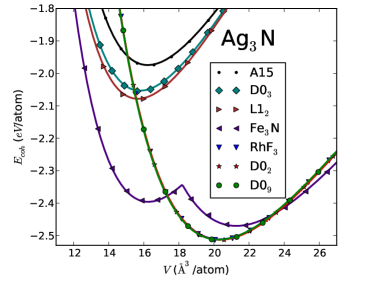
Figure 1: (Color online.) Cohesive energy $E_{\text{coh}}(eV/\text{atom})$ versus atomic volume $V$ (ų/atom) for Ag₃N in seven different structural phases.

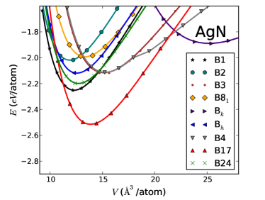
Figure 2: (Color online.) Cohesive energy $E_{\text{coh}}(eV/\text{atom})$ versus atomic volume $V$ (ų/atom) for AgN in nine different structural phases.

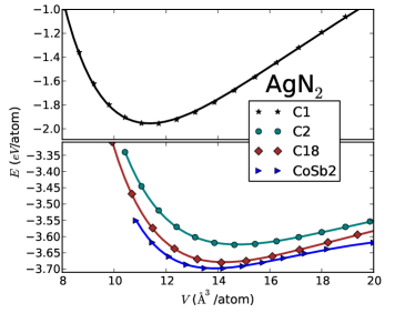
Figure 3: (Color online.) Cohesive energy $E_{coh}(eV/\text{atom})$ versus atomic volume $V(\AA^{3}/\text{atom})$ for AgN₂ in four different structural phases.

Table 1: Calculated and experimental zero-pressure properties of the twenty studied phases of Ag₃N, AgN and AgN₂: Lattice constants ($a(\text{\AA})$, $b(\text{\AA})$, $c(\text{\AA})$, $\alpha(^{\circ})$ and $\beta(^{\circ})$), equilibrium atomic volume $V_{0}(\text{\AA}^{3}/$atom$)$, cohesive energy $E_{\text{coh}}(eV/$atom$)$, bulk modulus $B_{0}(GPa)$ and its pressure derivative $B_{0}^{\prime}$, and formation energy $E_{f}(eV/\text{atom})$. The presented data are of the current work (Pres.), experimentally reported (Expt.) and of previous calculations (Comp.).

Structure		$a(\AA)$	$b(\AA)$	$c(\AA)$	$\alpha(^{\circ})$ or $\beta(^{\circ})$	$V_{0}(\AA^{3}/$atom$)$	$E_{\text{coh}}(eV/\text{atom})$	$B_{0}(\text{GPa})$	$B_{0}^{\prime}$	$E_{f}(eV/\text{atom})$
Ag
A1	Pres.	$4.164$	–	–	–	$18.06$	$-2.484$	$88.188$	$5.793$
	Expt.	($4.08570\pm 0.00018$)	–	–	–		$-2.95$	$100.7$, $101$	$6.12$
	Comp.	$4.01$	–	–	–		$-3.59$, $-2.66$,	$142$	$5.00$, $5.70$,
							$-2.67$		$5.97$
Ag3N
D03	Pres.	$6.322$	–	–	–	$15.79$	$-2.055$	$98.356$	$5.457$	$1.107$
A15	Pres.	$5.065$	–	–	–	$16.24$	$-1.976$	$92.280$	$5.470$	$1.186$
D09	Pres.	$4.328$	–	–	–	$20.27$	$-2.513$	$71.980$	$5.386$	$0.649$
	Comp.	$3.995$, $4.169$, $4.292$	–	–	–			$95.7$, $87.1$
L12	Pres.	$3.972$	–	–	–	$15.67$	$-2.081$	$100.743$	$5.530$	$1.081$
D02	Pres.	$8.662$	–	–	–	$20.31$	$-2.514$	$72.230$	$5.335$	$0.648$
$\epsilon$-Fe3N	Pres.	$5.967$	–	$5.560$	–	$21.43$	$-2.469$	$64.737$	$2.335$	$0.692$
RhF3	Pres.	$6.126$	–	–	$\alpha=59.989$	$20.31$	$-2.514$	$72.237$	$5.396$	$0.648$
fcc	Expt.	$4.369$, $4.29$, $4.378$	–	–						$2.587\pm 0.364$
AgN
B1	Pres.	$4.617$	–	–	–	$12.30$	$-2.253$	$147.600$	$5.145$	$1.587$
	Comp.	$4.57$, $4.506$, $4.619$	–	–	–			$219.2$, $162.3$	$4.653$
		$4.476$, $4.606$	–	–	–			$197.18$, $147.40$	$4.883$
B2	Pres.	$2.873$	–	–	–	$11.86$	$-2.021$	$146.157$	$5.260$	$1.819$
	Comp.	$2.833$, $2.806$, $2.876$	–	–	–			$138.96$	$4.823$
		$2.78$, $2.87$	–		–			$204.10$	$5.451$
B3	Pres.	$4.950$	–	–	–	$15.16$	$-2.122$	$109.639$	$5.210$	$1.718$
	Comp.	$4.88$, $4.816$, $4.946$	–	–	–			$100.11$	$5.825$
		$4.79$, $4.94$	–	–	–			$151.05$	$4.542$
B81	Pres.	$3.544$	–	$4.929$	–	$13.40$	$-1.996$	$130.485$	$5.240$	$1.844$
B${}_{\text{k}}$	Pres.	$3.521$	–	$9.368$	–	$25.15$	$-1.891$	$57.077$	$5.110$	$1.949$
B${}_{\text{h}}$	Pres.	$3.096$	–	$3.023$	–	$12.55$	$-2.121$	$141.385$	$5.285$	$1.719$
B4	Pres.	$3.501$	–	$5.734$	–	$15.22$	$-2.113$	$105.992$	$5.467$	$1.727$
	Comp.	$3.41$, $3.54$	–	$5.52$, $5.69$	–			$143.68$, $110.12$	$4.82$, $4.663$
B17	Pres.	Pres. $3.158$	–	$5.560$	–	$13.86$	$-2.517$	$132.556$	$5.185$	$1.323$
B24	Pres.	$4.337$	$4.601$	$5.091$	–	$12.70$	$-2.202$	$138.704$	$5.132$	$1.638$
AgN2
C1	Pres.	$5.157$	–	–	–	$11.43$	$-1.959$	$164.844$	$4.996$	$2.333$
	Comp.	$5.124$, $5.055$, $5.172$	–	–	–			$181.3$, $164.5$
		$5.013$, $5.141$	–	–	–			$215$, $164$
C2	Pres.	$5.617$	–	–	–	$14.77$	$-3.626$	$30.058$	$6.894$	$0.666$
C18	Pres.	$3.440$	$4.513$	$5.508$	–	$14.25$	$-3.680$	$35.878$	$7.269$	$0.612$
CoSb2	Pres.	$5.976$	$5.651$	$10.261$	$\beta=151.225$	$13.90$	$-3.699$	$35.117$	$7.822$	$0.593$

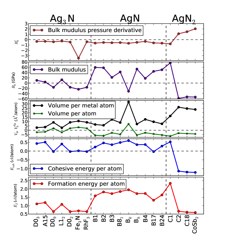
Figure 4: (Color online.) Calculated equilibrium properties of the twenty studied phases of silver nitrides. All quantities are given relative to the corresponding ones of the fcc crystalline elemental silver given in the first row of Table 1. The vertical dashed lines separate between the different stoichoimetries.

Considering $E_{\text{coh}}$ in the Ag₃N series, Fig. 1 shows clearly that the $E(V)$ relations of Ag₃N in D0₉, D0₂ and RhF₃ phases are almost identical, corresponding to equilibrium cohesive energy (Table 1) of $-2.513$, $-2.514$ and $-2.514\;\;eV/\text{atom}$, respectively. This behavior in the EOS could be traced back to the structural relationships between these three structures, since both D0₂ and RhF₃ can simply be derived from the more symmetric D0₉ (see Ref. Suleiman_PhD_arXiv2012_copper_nitrides_article, and references therein). These structural relations may reflect in the EOS’s and in other physical properties, and the three phases may co-exist during the Ag₃N synthesis process. Relative to the elemental Ag, these three phases tend not to change the $E_{\text{coh}}$ (Fig. 4), lowering it only by $\sim 0.03\;eV/\text{atom}$, as can been seen from Table 1. It may be worth to mention here that the simple cubic D0₉ phase is the stable phase of the synthesized Cu₃N the_first_Cu3N_1939_exp ; Cu3N_1996_comp .

The odd behavior of the EOS of Ag₃N(Fe₃N) with the existence of two minima (Fig. 1) shows that the first minima (to the left) is a metastable local minimum that cannot be maintained as the system is decompressed. Ag ions are in the $6g$ Wyckoff positions: $(x,0,0),(0,x,0),(-x,-x,0),(-x,0,\frac{1}{2}),(0,-x,\frac{1}{2})$ and $(x,x,\frac{1}{2})$; with $x\sim\frac{1}{3}$ to the left of the potential barrier (represented by the sharp peak at $\sim 18.2\;\text{\AA}^{3}/\text{atom}$), and $x=\frac{1}{2}$ to the right of the peak. It may be relevant to mention here that Cu₃N(Fe₃N) was found to behave in a similar manner Suleiman_PhD_arXiv2012_copper_nitrides_article .

The crossings of the less stable A15, D0₃ and L1₂ EOS curves with the more stable D0₉, D0₂ and RhF₃ ones at the left side of their equilibrium points reveals pressure-induces phase transitions from the latter phases to the former. To show this, we plotted the corresponding relation between enthalpy $H=E(V)+PV$ and the imposed pressure $P$ in Fig. 5. Since D0₉, D0₂ and RhF₃ phases have identical $E(V)$ curves, the corresponding $H(P)$ curves are also identical. Hence, only the $H(P)$ of D0₉ is displayed in Fig. 5. A point where the enthalpies of two phases are equal determine the phase transition pressure $P_{t}$; and, indeed, the direction of the transition is from the higher $H$ to the lower $H$ Grimvall . As depicted in Fig. 5, $P_{t}(\text{D0}_{9}\rightarrow\text{L1}_{2})=17.8\;\text{GPa}$, $P_{t}(\text{D0}_{9}\rightarrow\text{D0}_{3})=19.5\;\text{GPa}$ and $P_{t}(\text{D0}_{9}\rightarrow\text{A15})=26.0\;\text{GPa}$. Thus, D0₉, D0₂ and RhF₃ would not survive behind these $P_{t}$’s and A15, D0₃ and L1₂ are preferred at high pressure.

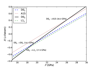
Figure 5: (Color online.) Enthalpy $H$ vs. pressure $P$ equation of state (EOS) for some Ag₃N phases in the range where D0₉ $\rightarrow$ A15, D0₉ $\rightarrow$ D0₃ and D0₉ $\rightarrow$ L1₂ phase transitions occur.

Fig. 4 reveals that the AgN group contains the least stable phase among all the twenty studied phases: the hexagonal B${}_{\text{k}}$. Fig. 2 and Table 1 show that the simple tetragonal structure of cooperite (B17) is the most stable phase in this AgN series. In fact, one can see from Fig. 4 and Table 1 that all the considered AgN phases possess less binding than their parent Ag(fcc), except AgN(B17) which is slightly more stable, with $0.033\;eV/\text{atom}$ lower $E_{\text{coh}}$. It is interesting to notice that AgN(B17) is $\sim 0.003\;eV/\text{atom}$ more stable than the Ag₃N most stable phases. Moreover, this B17 structure was theoretically predicted to be the ground-state structure of CuN Suleiman_PhD_arXiv2012_copper_nitrides_article , AuN Suleiman_PhD_SAIP2012_gold_nitrides_article , PdN Suleiman_PhD_SAIP2012_palladium_nitrides_article and PtN PtN_2006_comp_B17_structure_important .

Using the full-potential (linearized) augmented plane waves plus local orbitals (FP-LAPW+lo) method within LDA and within GGA, Kanoun and Said CuN_AgN_AuN_2007_comp studied the $E(V)$ EOS for AgN in the B1, B2, B3 and B4 structures. The equilibrium energies they obtained from the $E(V)$ EOS revealed that B1 is the most stable phase, and the relative stability they arrived at is in the order B1–B3–B4–B2, with a significant difference in total energy between B3 and B4 (see Fig. 2(b) in that article). Within this subset of structures, the numerical values of $E_{\text{coh}}$ in Table 1 do have the same order. However, the difference between the equilibrium $E_{\text{coh}}$(B3) and $E_{\text{coh}}$(B4) is only $\sim 0.009\;eV$, and the $E(V)$ EOS of B3 and B4 match/overlap over a wide range of volumes around the equilibrium point. This discrepancy may be attributed to the unphysical/ill-defined measure of stability that Kanoun and Said used, the total energy, while the number of the AgN formula units per unit cell in the B4 structure differs from that in the others. Nevertheless, it may be worth mentioning here that AgN(B3) was found to be elastically unstable AgN_AgN2_Ag2N_Ag3N_2010_comp .

In the CuN₂ nitrogen-richest phase series, we can see from Table 1 and from Fig. 4 that the phases of this group are significantly more stable than all the other studied phases, except C1, which is, in contrast, the second least stable among the twenty studied phases, with $0.017\;eV/\text{atom}$ more than AgN(B${}_{\text{k}}$). From Fig. 3, Fig. 4 and Table 1, one can see that in this series, the lower the structural symmetry, the more stable is the phase. It was found that CuN₂ phases have the same trend Suleiman_PhD_arXiv2012_copper_nitrides_article .

Comparing the relative stability of Ag₃N, AgN and AgN₂, we find from Table 1 and from Fig. 4 that AgN₂ in its least symmetric phase, the simple monoclinc structure of CoSb₂, is the most energetically stable phase with $E_{\text{coh}}=-3.699$ $eV/\text{atom}$.

III.2 Volume per Atom and Lattice Parameters

The numerical values of the lattice parameters and the average equilibrium volume per atom $V_{0}$ for the twenty modifications are presented in Table 1. The middle subwindow of Fig. 4 depicts the $V_{0}$ values relative to the Ag(fcc). To measure the average of the Ag–Ag bond length in the silver nitride, the equilibrium average volume per Ag atom ($V_{0}^{Ag}$), which is simply the ratio of the volume the unit cell to the number of Ag atoms in the unit cell, is visualized in the same subwindow.

From the $V_{0}$ curve in Fig. 4, we can see that, all AgN and AgN₂ modifications, except the open AgN(B${}_{\text{k}}$) phase, decrease $V_{0}$; while the Ag₃N phases tend, on average, not to change the number density of the parent Ag(A1).

On the other hand, the $V_{0}^{\text{Ag}}$ curve in Fig. 4 reveals that, relative to the elemental Ag and to each other, $V_{0}^{Ag}$ tends to increase with the increase in the nitrogen content. Thus, in all these nitrides, the introduced N ions displace apart the ions of the host lattice causing longer Ag-Ag bonds than in the elemental Ag. This cannot be seen directly from the $V_{0}$ values depicted in the same figure.

For AgN in the B1, B2, B3 and B4 structures, Kanoun and Said (Ref. CuN_AgN_AuN_2007_comp, described in Sec. III.1 above) obtained GGA equilibrium lattice parameters which are in very good agreement with ours. Their obtained LDA lattice parameter values show the common underestimation with respect to their and our GGA values (see Table 1).

Gordienko and Zhuravlev AgN_AgN2_Ag2N_Ag3N_2010_comp studied the structural, mechanical and electronic properties of AgN(B1) , AgN(B2), AgN(B3), AgN₂(C1) and Ag₃N(D0₉) cubic phases. Their DFT calculations were based on pseudopotential (PP) method within LDA, and on linear combinations of atomic orbitals (LCAO) method within both LDA and GGA. For comparison, some of their findings are included in Table 1. Within the parameter subspace they considered, our GGA values of the $a$ lattice parameter agree very well with theirs. On the other hand, although their PP $a$ values are closer to the GGA ones (ours and theirs), all their LDA values are less than the GGA ones. This confirms the well-known behavior of LDA compared to GGA accurate_GGA_2006 ; GGA_vs_LDA_2004 ; Ch1_in_Primer_in_DFT_2003 . Gordienko and Zhuravlev also found that the Ag–Ag interatomic distance increases in the order Ag₃N–AgN–AgN₂. This agrees with the general trend shown in Fig. 4, since the $V_{0}^{Ag}$ curve shows an average increase in the same direction.

III.3 Bulk Modulus and its Pressure Derivative

Fig. 4 reveals that Ag₃N phases tend, on average, to preserve the $B_{0}$ value of the parent Ag(A1). Increasing the nitrogen content to get AgN phases will increase the $B_{0}$ value of the parent Ag(A1), except in the case of B_k. While the nitrogen in AgN₂ tends to lower the $B_{0}$ value of the parent Ag(A1), the cubic C1 phase posses the highest $B_{0}$ value. This could be seen from Fig. 3, where the curvature of the $E_{\text{coh}}(V)$ curve of C1 is higher compared to the shallow minima of the C2, C18 and CoSb₂ curves.

From the definition of the equilibrium bulk modulus (Eq. 5), one would expect $B_{0}$ to increase as $E_{\text{coh}}$ or $V_{0}$ decreases. This is because of the minus sign of the former and the inverse proportionality of the latter. That is, roughly speaking, the $B_{0}$ curve should have a mirror reflection-like behavior with respect to the $E_{\text{coh}}$ and $V_{0}$ curves. Nevertheless, if $E_{\text{coh}}$ or $V_{0}$ are increasing and the other is decreasing, then the dominant net effect will be of the one with the higher change . For example, Fig. 4 shows that in going from D0₃ to A15, both $E_{\text{coh}}$ and $V_{0}$ increase resulting in a negative change in $B_{0}$. In going from A15 to D0₉, $E_{\text{coh}}$ is decreasing while $V_{0}$ is increasing, but, in the end, the latter won the competition and lowered the value of $B_{0}$. This argument stays true throughout the three series. When there is no significant change in both $E_{\text{coh}}$ and $V_{0}$, there is no significant change in $B_{0}$. This is the case when one goes from C18 to CoSb₂. A close look at the $B_{0}$ curve in Fig. 4, reveals that the huge decrease in $E_{\text{coh}}$ between C1 and C2 defeats the relatively small increase in $V_{0}$. This is simply because, according to Eq. 5, the value of $B_{0}$ is proportional to the absolute change in $E_{\text{coh}}$, while it is far more sensitive to any change in $V_{0}$ because it is proportional to $(\Delta V_{0})^{-1}$.

It is common to measure the pressure dependence of $B_{0}$ by its derivative $B^{\prime}_{0}$ (Eq. 6). Fig. 4 shows that the $B_{0}$ value of the C2, C18 and CoSb₂ phases increases as these phases are put under pressure. While the $B_{0}$ values of the rest of the phases shows very low sensitivity to pressure and they tend to slightly lower the bulk modulus, the Fe₃N phase is the most sensitive phase and tends to significantly lower its $B_{0}$ upon application of pressure. This high sensitivity may indicate that the corresponding minimum on the potential surface is not global, but another local minimum as the one at $16.2\;\AA^{3}/\text{atom}$ (Fig. 1).

From the elastic constants they obtained, Gordienko and ZhuravlevAgN_AgN2_Ag2N_Ag3N_2010_comp calculated the corresponding macroscopic bulk moduli (included in Table 1). They found the highest LDA $B_{0}$ value for AgN(B1) among all phases they considered, but, in agreement with the present work, they obtained the highest GGA $B_{0}$ value for AgN₂(C1). Since LDA relative to GGA overestimates $E_{\text{coh}}$ and thus underestimates $V_{0}$, each of these two factors (see Subsection III.3) would separately lead to the odd LDA value of $219.2$ GPa which they obtained. Nevertheless, due to this fact, Gordienko and Zhuravlev argued that one should consider the LDA and GGA average value of $B_{0}$.

III.4 Formation Energies

Formation energies in the present work are used as a measure of the relative thermodynamic stabilities of the phases under consideration. That is, the lower the formation energy, the lower the tendency to dissociate back into the constituent components Ag and N₂.

The obtained formation energies $E_{f}$ of the twenty relaxed phases are given in Table 1 and depicted graphically in Fig. 4. The latter shows that, relative to each other and within each series, the formation energy $E_{f}$ (defined by Eqs. 7 and II.4) of the studied phases has the same trend as the cohesive energy. That is, all phases have the same relative stabilities in the $E_{f}$ space as in the $E_{\text{coh}}$ space. However, while Ag₃N phases tend to have equal $E_{\text{coh}}$ as the AgN phases, all Ag₃N modifications have a lower $E_{f}$ than the AgN ones. Hence, silver nitride is more likely to be formed in the former stoichiometry. However, all the twenty obtained $E_{f}$ values are positive; which, in principle, means that all these phases are thermodynamically unstable (endothermic) .

Some of the experimental values of $E_{f}$ for the synthesized Ag₃N phase (which is claimed to be in an fcc structure) are $+199\;\text{kJ/mol}$ Juza_n_Hahn_1940 = $2.062\;eV/\text{atom}$, $+230\;\text{kJ/mol}$ Anderson_n_Parlee_1970_exp = $2.384\;eV/\text{atom}$, $+255\;\text{kJ/mol}$ German_Ag3N_structure_1949_exp = $2.643\;eV/\text{atom}$ and $(+314.4\mp 2.5)\;\text{kJ/mol}$ Ag3N_1991_exp = $(3.25853\pm 0.02591)\;eV$; with an average value of $2.587\pm 0.364\;eV$. Among the considered phases in the present work, there is only one phase wich has $E_{f}$ value that fits in this range, the AgN₂(C1). Interestingly, this C1 structure has an fcc underlying Bravia lattice; however, the chemical formula differs from that of the synthesized phase.

III.5 Electronic Properties

The DFT(GGA) calculated band diagrams (i.e. $\epsilon_{i}^{\sigma}(\mathbf{k})$ curves) and spin-projected total and orbital resolved (i.e. partial) density of states (DOS) of the most stable phases: D0₉, RhF₃, D0₂, B17, and C18 are presented in Figs. 6, 7, 8, 9 and 10, respectively. Spin-projected total density of states (TDOS) are shown in sub-figure (b) in each case. In all the six considered cases, electrons occupy the spin-up and spin-down bands equally, resulting in zero spin-polarization density of states: $\zeta(\epsilon)=n_{\uparrow}(\epsilon)-n_{\downarrow}(\epsilon)$. Thus, it is sufficient only to display spin-up (or spin-down) density of states (DOS) and spin-up (or spin-down) band diagrams. In order to investigate the details of the electronic structure of these phases, energy bands are plotted along densely sampled high-symmetry string of neighboring $\mathbf{k}$-points. Moreover, to extract information about the orbital character of the bands, the Ag($s,p,d$) and N($s,p$) partial DOS are displayed at the same energy scale.

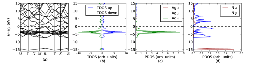
Figure 6: (Color online.) DFT calculated electronic structure for Ag₃N in the D0₉ structure: (a) band structure along the high-symmetry $\mathbf{k}$-points which are labeled according to Ref. [Bradley, ]. Their coordinates w.r.t. the reciprocal lattice basis vectors are: $M(0.5,0.5,0.0)$, $\Gamma(0.0,0.0,0.0)$, $X(0.0,0.5,0.0)$, $R(0.5,0.5,0.5)$; (b) spin-projected total density of states (TDOS); (c) partial density of states (PDOS) of Ag($s,p,d$) orbitals in Ag₃N; and (d) PDOS of N($s,p$) orbitals in Ag₃N,.

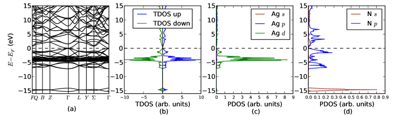
Figure 7: (Color online.) DFT calculated electronic structure for Ag₃N in the RhF₃ structure: (a) band structure along the high-symmetry $\mathbf{k}$-points which are labeled according to Ref. [Bradley, ]. Their coordinates w.r.t. the reciprocal lattice basis vectors are: $F(0.5,0.5,0.0)$, $Q(0.375,0.625,0.0)$, $B(0.5,0.75,0.25)$, $Z(0.5,0.5,0.5)$, $\Gamma(0.0,0.0,0.0)$, $L(0.0,0.5,0.0)$, $Y(0.25,0.5,-.25)$, $\Sigma(0.0,0.5,-.5)$; (b) spin-projected total density of states (TDOS); (c) partial density of states (PDOS) of Ag($s,p,d$) orbitals in Ag₃N; and (d) PDOS of N($s,p$) orbitals in Ag₃N.

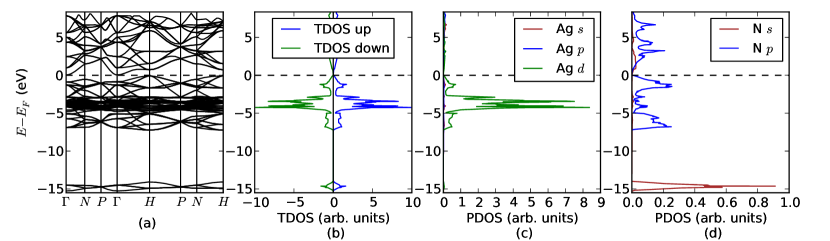
Figure 8: (Color online.) DFT calculated electronic structure for Ag₃N in the D0₂ structure: (a) band structure along the high-symmetry $\mathbf{k}$-points which are labeled according to Ref. [Bradley, ]. Their coordinates w.r.t. the reciprocal lattice basis vectors are: $\Gamma(0.0,0.0,0.0)$, $N(0.0,0.0,0.5)$, $P(0.25,0.25,0.25)$, $H(0.5,-.5,0.5)$; (b) spin-projected total density of states (TDOS); (c) partial density of states (PDOS) of Ag($s,p,d$) orbitals in Ag₃N; and (d) PDOS of N($s,p$) orbitals in Ag₃N.

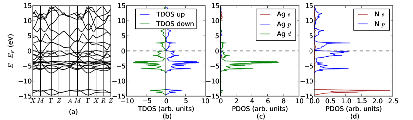
Figure 9: (Color online.) DFT calculated electronic structure for AgN in the B17 structure: (a) band structure along the high-symmetry $\mathbf{k}$-points which are labeled according to Ref. [Bradley, ]. Their coordinates w.r.t. the reciprocal lattice basis vectors are: $X(0.0,0.5,0.0)$, $M(0.5,0.5,0.0)$, $\Gamma(0.0,0.0,0.0)$, $Z(0.0,0.0,0.5)$, $A(0.5,0.5,0.5)$, $R(0.0,0.5,0.5)$; (b) spin-projected total density of states (TDOS); (c) partial density of states (PDOS) of Ag($s,p,d$) orbitals in AgN; and (d) PDOS of N($s,p$) orbitals in AgN.

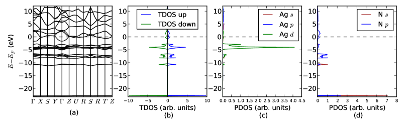
Figure 10: (Color online.) DFT calculated electronic structure for AgN₂ in the C18 structure: (a) band structure along the high-symmetry $\mathbf{k}$-points which are labeled according to Ref. [Bradley, ]. Their coordinates w.r.t. the reciprocal lattice basis vectors are: $\Gamma(0.0,0.0,0.0)$, $X(0.0,0.5,0.0)$, $S(-.5,0.5,0.0)$, $Y(-.5,0.0,0.0)$, $Z(0.0,0.0,0.5)$, $U(0.0,0.5,0.5)$, $R(-.5,0.5,0.5)$, $T(-.5,0.0,0.5)$; (b) spin-projected total density of states (TDOS); (c) partial density of states (PDOS) of Ag($s,p,d$) orbitals in AgN₂; and (d) PDOS of N($s,p$) orbitals in AgN₂.

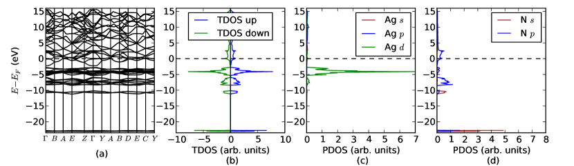
Figure 11: (Color online.) DFT calculated electronic structure for AgN₂ in the CoSb₂ structure: (a) band structure along the high-symmetry $\mathbf{k}$-points which are labeled according to Ref. [Bradley, ]. Their coordinates w.r.t. the reciprocal lattice basis vectors are: $\Gamma(0.0,0.0,0.0)$, $B(-.5,0.0,0.0)$, $A(-.5,0.5,0.0)$, $E(-.5,0.5,0.5)$, $Z(0.0,0.0,0.5)$, $Y(0.0,0.5,0.0)$, $D(-.5,0.0,0.5)$ and $C(0.0,0.5,0.5)$; (b) spin-projected total density of states (TDOS); (c) partial density of states (PDOS) of Ag($s,p,d$) orbitals in AgN₂; and (d) PDOS of N($s,p$) orbitals in AgN₂.

Fig. 6(a) shows the band structure $\epsilon_{i}^{\sigma}(\mathbf{k})$ of Ag₃N(D0₉). With its valence band maximum (VBM) at $(R,-0.086\;eV)$ and its conduction band minimum (CBM) at $(\Gamma,0.049\;eV)$, Ag₃N(D0₉) presents a semiconducting character with a narrow indirect band gap $E_{g}$ of $0.134\;eV$. From sub-figures 6(c) and (d), it is seen clearly that the Ag($d$)-N($p$) mixture in the region from $-7.286\;eV$ to $-0.086\;eV$ beneath $E_{F}$, with two peaks: a low density peak around $1.5\;eV$ and a high density peak around $4.0\;eV$ steaming mainly from the bands of silver $d$ electrons.

Our obtained PDOS, TDOS and band structure of Ag₃N(D0₉) agree qualitatively well with Gordienko and Zhuravlev AgN_AgN2_Ag2N_Ag3N_2010_comp ; however, using LCAO method within GGA, the value of the indirect $E_{g}$ of Ag₃N(D0₉) they predicted is $0.25\;eV$.

To the best of our knowledge, there is no experimentally reported $E_{g}$ value for Ag₃N. However, Tong Ag_Pd_Au_nitrides_PhD_thesis_2010_exp prepared Ag_3+xN samples, and carried out XRD measurements to confirm the fcc symmetry of the prapared samples. Using a TB-LMTO code within LDA, Tong then calculated the band structure of Ag₃N and obtained an indirect energy gap of $1.35\;eV$. Nevertheless, we could not figure out the positions of the N ions Tong’s model.

It is a well known drawback of Kohn-Sham DFT-based calculations to underestimate the band gap. Thus the more demanding $GW$ calculations were carried out, and the obtained $E_{g}$ value will be presented in Sec. III.6.

Calculated electronic properties of Ag₃N(D0₂) are displayed in Fig. 8. sub-figure 8(a) shows the energy bands $\epsilon_{i}^{\sigma}(\mathbf{k})$ of Ag₃N(D0₂). With its valence band maximum (VBM) at $(H,-0.091\;eV)$ and its conduction band minimum (CBM) at $(\Gamma,0.039\;eV)$, Ag₃N(D0₉) presents semiconducting character with a narrow indirect band gap $E_{g}$ of $0.130\;eV$. From sub-figures 8(c) and (d), one can notice clearly the Ag($d$)-N($p$) mixture in the region from $-7.249\;eV$ to $-0.091\;eV$ below $E_{F}$, with two peaks: a low density peak around $-1.3\;eV$ steaming from an almost equal mixture of Ag($d$) and N($p$), and a high density peak around $-4.3\;eV$ steming mainly from the bands of silver $d$ electrons plus a relatively very low contribution from the N($p$) states.

Fig. 7 depicts the band diagram and DOS’s of Ag₃N(RhF₃). In contrast to Ag₃N(D0₉) and Ag₃N(D0₂), sub-figure 7(a) shows that Ag₃N(RhF₃) is a semiconductor with a narrow direct band gap of $0.129\;eV$ of width located at $\Gamma$ point. The VBM is at $-0.089\;eV$ and the CBM is at $0.040\;eV$. From sub-figures 7(c) and (d), one can see the Ag($d$)-N($p$) mixture is in the region from $-7.286\;eV$ to $-0.089\;eV$ beneath $E_{F}$, with two peaks: a low density peak around $-1.366\;eV$ steaming from an almost equal mixture of Ag($d$) and N($p$), and a high density peak around $-4.382\;eV$ steaming mainly from the bands of silver $d$ electrons plus a relatively very low contribution from the N($p$) states.

The relationship between D0₉, D0₂ and RhF₃ structures manifests itself in many common features between the electronic structure of these three Ag₃N nitrides: (i) equal $E_{g}$ of $\sim 0.13\;eV$; (ii) a deep bound band around $\thicksim-14.6\;eV$ below $E_{F}$ consists mainly of the N$(2s)$ states; (iii) a broad valence band with $\sim 7.2\;eV$ of width that comes mostly from the $4d$ electrons of Ag plus a very small contribution from N$(2p)$; and (iv) the relatively low TDOS of the conduction bands.

Energy bands $\epsilon_{i}^{\sigma}(\mathbf{k})$, total density of states (TDOS) and partial (orbital-resolved) density of states (PDOS) of AgN(B17) are shown in Figs. 9. It is clear that AgN(B17) would be a true metal at its equilibrium. The major contribution to the very low TDOS around Fermi energy $E_{F}$ comes from the $2p$ states of the N atoms as it is evident from sub-figure 9(d). Beneath $E_{F}$ lies a band with $\sim 7.3\;eV$ of width, in which the main contribution is due to the Ag($4d$) states plus a small contribution from the N($2p$) states. While the N($2s$) states dominate the deep lowest region around $13.5\;eV$, the low density unoccupied bands stem mainly from the N($2p$) states. The Fermi surface crosses two partly occupied bands: a lower one in the $X$-$M$, $\Gamma$-$Z$-$A$ and $\Gamma$-$X$-$R$ directions, and a higher band in the $X$-$M$-$\Gamma$ and $M$-$A$ directions. Thus, $E_{F}$ is not a continuous surface contained entirely within the first BZ.

It may be worth mentioning here that AgN(B1) CuN_AgN_AuN_2007_comp ; AgN_2008_comp and AgN(B3) CuN_AgN_AuN_2007_comp ; PdN_AgN_2007_comp phases were also theoretically predicted to be metallic.

Although AgN₂(CoSb₂) is the most stable phase, but the difference in cohesive energy between AgN₂(CoSb₂) and AgN₂(C18) is less than $0.02\;eV/\text{atom}$, and we decided to examine the electronic structure of both phases. With $E_{F}$ crossing the finite TDOS, Fig. 10 shows that AgN₂(C18) is metallic at $0\;K$. The orbital resolved DOS’s reveal that the major contribution to the low TDOS at $E_{F}$ comes from the N($2p$) states with tiny contributions from the $5s$, $4d$ and $3p$ states of Ag, respectively. As one can see from sub-figure 10(a), the $E_{F}$ surface crosses the edges of the first Brillouin zone in the $Z$-$U$-$R$-$S$-$T$-$X$ and $T$-$Z$ directions.

The calculated electronic properties of AgN₂(CoSb₂) are displayed in Fig. 11. Band structure, TDOS and orbital resolved DOS’s have almost the same features as the corresponding ones of AgN₂(C18). It may be worth to mention here that C1 phase of AgN₂ was also theoretically predicted to be metallic AgN_AgN2_Ag2N_Ag3N_2010_comp .

Compared to the metallic AgN(B17), three new features of these 1:2 nitrides are evident: (i) Deep at $\sim-22.7\;eV$ there is a highly-localized mixture of the N($s$)-N($p$) states. However, the variation in N($2s$) energy with respect to k is smaller than the variation of N($2p$) states, resulting in a narrower and higher PDOS. (ii) Below the band that is crossed by $E_{F}$ there are four bands separated by $\sim 11.4\;eV$, $\sim 1.6\;eV$, $\sim 0.38\;eV$ and $\sim 0.28\;eV$ energy gaps, respectively. (iii) The very tiny contribution of the N($p$) states to the N($2p$)-Ag($4d$) band.

A common feature of all the studied cases is that Ag($p$)-orbitals do not contribute significantly to the hybrid bands. Another common feature is the highly structured, intense and narrow series of peaks in the TDOS valance band corresponding to the superposition of N($2p$) and Ag($4d$) states. In their $\mathbf{k}$-space, Ag($4d$) energies show little variation with respect to $\mathbf{k}$; hence the Van Hove singularities-like sharp features.

To summarize, we have found that the most stable phases of AgN and AgN₂ are metallic, while those of Ag₃N are semiconductors. A close look at Fig. 9 up to Fig. 6 reveals that as the nitrogen to silver ratio increases from $x=1$ to $x=1/2$, the TDOS at $E_{F}$ decreases; and by arriving at $x=1/3$ a gap opens. This finding agrees well with Gordienko and Zhuravlev AgN_AgN2_Ag2N_Ag3N_2010_comp . Moreover, it may be worth mentioning here that such behavior was theoretically predicted to be true for copper nitrides as well Suleiman_PhD_arXiv2012_copper_nitrides_article ; Cu3N_Cu4N_Cu8N_2007_comp .

III.6 Optical Properties

Fig. 12 depicts the $GW$ calculated real and imaginary parts of the frequency-dependent dielectric function $\varepsilon_{\text{RPA}}(\omega)$ of Ag₃N(D0₉) and the corresponding derived optical constants. The optical region is shaded in each sub-figure.

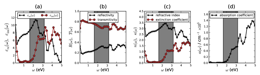
Figure 12: (Color online.) The $GW$ calculated frequency-dependent optical spectra of Ag₃N(D0₉): (a) the real $\varepsilon_{\text{re}}(\omega)$ and the imaginary $\varepsilon_{\text{im}}(\omega)$ parts of the dielectric function $\varepsilon_{\text{RPA}}(\omega)$; (b) reflectivity $R(\omega)$ and transmitivity $T(\omega)$; (c) refraction $n(\omega)$ and extinction $\kappa(\omega)$ coefficients; and (d) absorption coefficient $\alpha(\omega)$. The shaded area highlights the optical region.

The real part $\varepsilon_{\text{re}}(\omega)$ (sub-figure 12(a)) shows an upward trend before $\sim 2.3\;eV$, where it reaches its maximum value and generally decreases after that. The imaginary part $\varepsilon_{\text{im}}(\omega)$ (same sub-figure 12(a)) shows an upward trend before $\sim 1.0\;eV$ and it has three main peaks located at $\sim 2.6\;eV$ in the optical region, $\sim 3.3\;eV$ at the right edge of the optical region, and at $\sim 4.1\;eV$ in the UV range.

Calculated reflectivity $R(\omega)$ and transmitivity $T(\omega)$ are displayed in sub-figure 12(b). With $0.6\leq R(\omega)\leq 0.8$, it is evident that Ag₃N(D0₉) is a good reflector, specially in the red and the infrared regions. In the visible range, the maximum transmitivity $T(\omega)$ is at $\sim 2.54\;eV\equiv 489\;\text{nm}$, which is at the blue-green edge.

sub-figure 12(c) depicts the calculated refraction $n(\omega)$ and extinction $\kappa(\omega)$ coefficients. As they should, these two spectra have, in general, the same qualitative frequency dependence as the real $\varepsilon_{\text{re}}(\omega)$ and the imaginary $\varepsilon_{\text{im}}(\omega)$ dielectric functions, respectively.

From the absorption coefficient $\alpha\left(\omega\right)$ spectrum (sub-figure 12(d)), it can be seen that Ag₃N(D0₉) starts absorbing photons with $\sim 0.9\;eV$ energy. Hence, it is clear that $GW_{0}$ calculations give a band gap of $\sim 0.9\;eV$, which is a significant improvement over the value obtained from DFT. The non-vanishing $\alpha\left(\omega\right)$ in the whole optical region agrees with the experiment, since it may explain the observed black color of the synthesized Ag₃N.

To the best of our knowledge, the present work is the first trial to theoretically investigate the optical properties of silver nitride. However, for more accurate optical characterization (e.g. more accurate positions and amplitudes of the characteristic peaks), electron-hole excitations should be calculated. This can be done by evaluating the two-body Green function $G_{2}$ on the basis of our obtained GW one-particle Green function $G$ and QP energies, then solving the so-called Bethe-Salpeter equation, the equation of motion of $G_{2}$ DFT_GW_BSE_Electron-hole_excitations_and_optical_spectra_from_first_principles_2000 .

IV Conclusions

We have succesfully employed first-principles calculation methods to investigate the structural, stability, electronic and optical properties of Ag₃N, AgN and AgN₂. Within the accuracy of the employed methods, the obtained structural parameters, EOS, $B_{0}$, $B_{0}^{\prime}$ and electronic properties show good agreement with the few avialable previous calculations. On the other hand, our obtained results show, at least, partial agreement with three experimental facts: (i) the lattice parameter of Ag₃N(D0₉) is close to the experimentally reported one; (ii) the positive formation energies reveals the endothermic (unstable) nature of silver nitrides, and (iii) absorption spectrum explains its observed black color. Moreover, the present work may be considered as the first trial to theoretically investigate the optical properties of silver nitride. We hope that some of our obtained results will be confirmed in future experimentally and/or theoretically.

References

- (1) D. Åberg, P. Erhart, J. Crowhurst, J. M. Zaug, A. F. Goncharov, and B. Sadigh, Physical Review B 82, 104116 (Sep 2010), http://link.aps.org/doi/10.1103/PhysRevB.82.104116
- (2) X. P. Du and Y. X. Wang, Journal of Applied Physics 107, 053506 (2010), http://link.aip.org/link/?JAP/107/053506/1
- (3) M. G. Moreno-Armenta, W. L. Pérez, and N. Takeuchi, Solid State Sciences 9, 166 (2007), ISSN 1293-2558, http://www.sciencedirect.com/science/article/pii/S1293255806002858
- (4) R. Juza and H. Hahn, Zeitschrift für anorganische und allgemeine Chemie 241, 172 (1939), ISSN 1521-3749, http://dx.doi.org/10.1002/zaac.19392410204
- (5) M. S. H. Suleiman, M. P. Molepo, and D. P. Joubert, ArXiv e-prints(Nov. 2012), arXiv:1211.0179 [cond-mat.mtrl-sci]
- (6) Y. Du, A. Ji, L. Ma, Y. Wang, and Z. Cao, Journal of Crystal Growth 280, 490 (2005), ISSN 0022-0248, http://www.sciencedirect.com/science/article/pii/S0022024805004264
- (7) E. S. Shanley and J. L. Ennis, Industrial & Engineering Chemistry Research 30, 2503 (1991), http://pubs.acs.org/doi/pdf/10.1021/ie00059a023, http://pubs.acs.org/doi/abs/10.1021/ie00059a023
- (8) J. Tong, Darstellung, Strukturen und Eigenschaften ausgewählter Perowskit-Materialien und Molekülkristalle, Ph.D. thesis, Max-Planck-Institut für Festkörperforschung, Stuttgart (2010), http://elib.uni-stuttgart.de/opus/volltexte/2010/5816/
- (9) H. Hahn and E. Gilbert, Zeitschrift für anorganische Chemie 258, 77 (1949), ISSN 1521-3749, http://dx.doi.org/10.1002/zaac.19492580109
- (10) R. Anderson and N. Parlee, High Temperature Science 2, 289 (1970), http://www.osti.gov/energycitations/product.biblio.jsp?query_id=0&page=%0&osti_id=4085944
- (11) R. Juza and H. Hahn, Zeitschrift für anorganische und allgemeine Chemie 244, 133 (1940), ISSN 1521-3749, http://dx.doi.org/10.1002/zaac.19402440205
- (12) M. Haisa, Acta Crystallographica Section A 38, 443 (Jul 1982), http://dx.doi.org/10.1107/S0567739482000990
-
(13)
Ag3N, formerly termed fulminating
silver by its discoverers, can be formed from ammoniacal solutions of silver
oxide according to the following reaction
It can also be formed by means of other reactions Ag3N_1991_exp ; Ag_Pd_Au_nitrides_PhD_thesis_2010_exp .(17) - (14) J. L. Ennis and E. S. Shanley, Journal of Chemical Education 68, A6 (1991), http://pubs.acs.org/doi/pdf/10.1021/ed068pA6, http://pubs.acs.org/doi/abs/10.1021/ed068pA6
- (15) A. Gordienko and Y. Zhuravlev, Journal of Structural Chemistry 51, 401 (2010), ISSN 0022-4766, http://dx.doi.org/10.1007/s10947-010-0061-8
- (16) M. Kanoun and S. Goumri-Said, Physics Letters A 362, 73 (2007), ISSN 0375-9601, http://www.sciencedirect.com/science/article/pii/S0375960106015337
- (17) R. Yu and X. F. Zhang, Physical Review B 72, 054103 (Aug 2005), http://link.aps.org/doi/10.1103/PhysRevB.72.054103
- (18) A. F. Wells, Structural Inorganic Chemistry, 5th ed. (Oxford University Press, 1984) ISBN 9780198553700, http://books.google.co.za/books?id=lQfwAAAAMAAJ
- (19) U. von Barth and L. Hedin, Journal of Physics C: Solid State Physics 5, 1629 (Feb 1972), http://iopscience.iop.org/0022-3719/5/13/012/
- (20) M. Pant and A. Rajagopal, Solid State Communications 10, 1157 (1972), ISSN 0038-1098, http://www.sciencedirect.com/science/article/pii/0038109872909349
- (21) G. Kresse and J. Hafner, Physical Review B 47, 558 (Jan 1993), http://link.aps.org/doi/10.1103/PhysRevB.47.558
- (22) G. Kresse and J. Hafner, Physical Review B 49, 14251 (May 1994), http://link.aps.org/doi/10.1103/PhysRevB.49.14251
- (23) G. Kresse and J. Furthmüller, Computational Materials Science 6, 15 (1996), ISSN 0927-0256, http://www.sciencedirect.com/science/article/pii/0927025696000080
- (24) G. Kresse and J. Furthmüller, Physical Review B 54, 11169 (Oct 1996), http://link.aps.org/doi/10.1103/PhysRevB.54.11169
- (25) J. Hafner, Journal of Computational Chemistry 29, 2044 (2008), ISSN 1096-987X, http://dx.doi.org/10.1002/jcc.21057
- (26) G. Kresse and D. P. Joubert, Physical Review B 59, 1758 (Jan 1999), http://link.aps.org/doi/10.1103/PhysRevB.59.1758
- (27) W. Kohn and L. J. Sham, Physical Review 140, A1133 (Nov 1965), http://link.aps.org/doi/10.1103/PhysRev.140.A1133
- (28) H. J. Monkhorst and J. D. Pack, Physical Review B 13, 5188 (Jun 1976), http://link.aps.org/doi/10.1103/PhysRevB.13.5188
- (29) O. Jepson and O. Anderson, Solid State Communications 9, 1763 (1971), ISSN 0038-1098, http://www.sciencedirect.com/science/article/pii/0038109871903139
- (30) G. Lehmann and M. Taut, physica status solidi (b) 54, 469 (1972), ISSN 1521-3951, http://dx.doi.org/10.1002/pssb.2220540211
- (31) P. E. Blöchl, O. Jepsen, and O. K. Andersen, Physical Review B 49, 16223 (Jun 1994), http://link.aps.org/doi/10.1103/PhysRevB.49.16223
- (32) M. Methfessel and A. T. Paxton, Physical Review B 40, 3616 (Aug 1989), http://link.aps.org/doi/10.1103/PhysRevB.40.3616
- (33) J. P. Perdew, K. Burke, and M. Ernzerhof, Physical Review Letters 77, 3865 (Oct 1996), http://link.aps.org/doi/10.1103/PhysRevLett.77.3865
- (34) J. P. Perdew, K. Burke, and M. Ernzerhof, Physical Review Letters 78, 1396 (Feb 1997), http://link.aps.org/doi/10.1103/PhysRevLett.78.1396
- (35) M. Ernzerhof and G. E. Scuseria, The Journal of Chemical Physics 110, 5029 (1999), http://link.aip.org/link/?JCP/110/5029/1
- (36) A. D. Becke, Physical Review A 38, 3098 (Sep 1988), http://link.aps.org/doi/10.1103/PhysRevA.38.3098
- (37) J. P. Perdew, J. A. Chevary, S. H. Vosko, K. A. Jackson, M. R. Pederson, D. J. Singh, and C. Fiolhais, Physical Review B 46, 6671 (Sep 1992), http://link.aps.org/doi/10.1103/PhysRevB.46.6671
- (38) J. P. Perdew, J. A. Chevary, S. H. Vosko, K. A. Jackson, M. R. Pederson, D. J. Singh, and C. Fiolhais, Physical Review B 48, 4978 (Aug 1993), http://link.aps.org/doi/10.1103/PhysRevB.48.4978.2
- (39) P. E. Blöchl, Physical Review B 50, 17953 (Dec 1994), http://link.aps.org/doi/10.1103/PhysRevB.50.17953
- (40) F. Birch, Physical Review 71, 809 (Jun 1947), http://link.aps.org/doi/10.1103/PhysRev.71.809
- (41) M. Gajdoš and K. Hummer and G. Kresse and J. Furthmüller and F. Bechstedt, Physical Review B 73, 045112 (Jan 2006), http://link.aps.org/doi/10.1103/PhysRevB.73.045112
- (42) W. G. Aulbur, L. Jönsson, and J. W. Wilkins (Academic Press, 1999) pp. 1 – 218, http://www.sciencedirect.com/science/article/pii/S0081194708602489
- (43) J. Kohanoff, Electronic Structure Calculations for Solids and Molecules : Theory and Computational Methods (Cambridge University Press; Cambridge, 2006)
- (44) J. Harl, The Linear Response Function in Density Functional Theory: Optical Spectra and Improved Description of the Electron Correlation, Ph.D. thesis, University of Vienna (2008), http://othes.univie.ac.at/2622/
- (45) L. Hedin, Phys. Rev. 139, A796 (Aug 1965), http://link.aps.org/doi/10.1103/PhysRev.139.A796
- (46) G. Kresse, M. Marsman, and J. Furthmuller, “Vasp the guide,” (2011), available on-line at http://cms.mpi.univie.ac.at/vasp/vasp/. Last accessed October 2012.
- (47) M. Fox, Optical Properties of Solids, Oxford Master Series in Physics: Condensed Matter Physics (Oxford University Press, 2010) ISBN 9780199573363, http://books.google.co.za/books?id=-5bVBbAoaGoC
- (48) M. Dressel and G. Grüner, Electrodynamics of solids : optical properties of electrons in matter (Cambridge University Press, Cambridge New York, 2002) ISBN 0521592534
- (49) A. Miller, in Handbook of Optics, Volume 1: Fundamentals, Techniques, and Design, Optical Society of America (McGraw-Hill, Inc., New York, NY, USA, 2010) ISBN 0070479747, 9780070479746
- (50) J. Donohue, The structures of the elements, A Wiley-interscience publication (John Wiley & Sons Inc., 1974) ISBN 0471217883, http://books.google.co.za/books?id=Q-rvAAAAMAAJ
- (51) C. Kittel, Introduction to Solid State Physics, eigth ed. (John Wiley & Sons, Inc., 2005) ISBN 9780471415268, http://books.google.co.za/books?id=kym4QgAACAAJ
- (52) S. Raju, E. Mohandas, and V. Raghunathan, J. Phys. Chem Solids 58, 1367 (1997)
- (53) M. J. Mehl and D. A. Papaconstantopoulos, Physical Review B 54, 4519 (Aug 1996), http://link.aps.org/doi/10.1103/PhysRevB.54.4519
- (54) E. Zarechnaya, N. Skorodumova, S. Simak, B. Johansson, and E. Isaev, Computational Materials Science 43, 522 (2008), ISSN 0927-0256, http://www.sciencedirect.com/science/article/pii/S0927025608000037
- (55) U. Hahn and W. Weber, Physical Review B 53, 12684 (May 1996), http://link.aps.org/doi/10.1103/PhysRevB.53.12684
- (56) G. Grimvall, Thermophysical Properties of Materials (North Holland, 1986) http://books.google.co.za/books?id=TCWZlgbB3EEC
- (57) M. S. H. Suleiman and D. P. Joubert, in South African Institute of Physics 57 Annual Conference (SAIP 2012), No. 298 (2012) http://indico.saip.org.za/confSpeakerIndex.py?view=full&letter=s&confId%=14
- (58) M. S. H. Suleiman and D. P. Joubert, in South African Institute of Physics 57 Annual Conference (SAIP 2012), No. 299 (2012) http://indico.saip.org.za/confSpeakerIndex.py?view=full&letter=s&confId%=14
- (59) J. von Appen, M.-W. Lumey, and R. Dronskowski, Angewandte Chemie International Edition 45, 4365 (2006), ISSN 1521-3773, http://dx.doi.org/10.1002/anie.200600431
- (60) In their original articleCuN_AgN_AuN_2007_comp , Kanoun and Said stated that “… there are two atom in wurtzite unit cell, and one in all the other cases.” which is a clear typo!
- (61) Z. Wu and R. E. Cohen, Physical Review B 73, 235116 (Jun 2006), http://link.aps.org/doi/10.1103/PhysRevB.73.235116
- (62) V. N. Staroverov, G. E. Scuseria, J. Tao, and J. P. Perdew, Physical Review B 69, 075102 (Feb 2004), http://link.aps.org/doi/10.1103/PhysRevB.69.075102
- (63) J. P. Perdew and S. Kurth, in A Primer in Density Functional Theory, Lecture Notes in Physics (Springer, 2003) ISBN 9783540030836, http://books.google.co.za/books?id=mX793GABep8C
- (64) Since Eq. 5 does not refer to any stoichiometry or any species (that is, it does not consider the way that the change in energy or volume was done), we may take the change in volume (or energy) with respect to itself, with respect to the parent Ag(A1), or with respect to any of the other nineteen considered modifications.
- (65) Surely, this needs not to be so. Compare the definition 4 with the definition 7.
- (66) It is common that one obtains positive DFT formation energy for (even the experimentally synthesized) transition-metal nitrides. Moreover, the zero-pressure zero-temperature DFT calculations have to be corrected for the conditions of formation of these nitrides. Another source of this apparent shortcoming stems from the PBE-GGA underestimation of the cohesion in N2. We have discussed this point further in Ref. \rev@citealpnumSuleiman_PhD_arXiv2012_copper_nitrides_article.
- (67) C. J. Bradley and A. P. Cracknell, The Mathematical Theory of Symmetry in Solids: Representation Theory for Point Groups and Space Groups (Oxford: Clarendon Press, 1972)
- (68) D. Engin, C. Kemal, and C. Y. Oztekin, Chinese Physics Letters 25, 2154 (2008), http://stacks.iop.org/0256-307X/25/i=6/a=063
- (69) R. de Paiva, R. A. Nogueira, and J. L. A. Alves, Physical Review B 75, 085105 (Feb 2007), http://link.aps.org/doi/10.1103/PhysRevB.75.085105
- (70) M. G. Moreno-Armenta and G. Soto, Solid State Sciences 10, 573 (2008), ISSN 1293-2558, http://www.sciencedirect.com/science/article/pii/S1293255807002920
- (71) Recall that the optical region (i.e. the visible spectrum) is about which corresponds to .
- (72) M. Rohlfing and S. G. Louie, Physical Review B 62, 4927 (Aug 2000), http://link.aps.org/doi/10.1103/PhysRevB.62.4927