Relation between occupation in the first coordination shells and Widom line in Core-Softened Potentials

Abstract

Three core-softened families of potentials are checked for the presence of density and diffusion anomalies. These potentials exhibit a repulsive core with a softening region and at larger distances an attractive well. We found that the region in the pressure-temperature phase diagram in which the anomalies are present increases if the slope between the core-softened scale and the attractive part of the potential decreases. The anomalous region also increases if the range of the core-softened or of the attractive part of the potential decreases. We also show that the presence of the density anomaly is consistent with the non monotonic changes of the radial distribution function at each one of the two scales when temperature and density are varied. Then, using this anomalous behavior of the structure we show that the pressures and the temperatures in which the radial distribution functions of the two length scales are equal are identified with the Widom line.

I Introduction

Core-softened $(CS)$ potentials have been attracting attention due to their connections with the anomalous behavior of liquid systems including water. These potentials, U(r), exhibit a repulsive core with a softening region limited by $r_{1}<r<r_{2}$ where $d(rf)/dr>0$ with $f=-dU/dr$ [1]. Despite their simplicity, these models originate from the desire of constructing a simple two-body isotropic potential capable of describing the complicated features of systems interacting via anisotropic potentials  [2, 3, 4, 5, 6, 7, 8, 9, 10, 11, 12, 13, 14, 15, 16, 17, 18, 19, 20, 21, 22, 23, 24, 25, 26, 27]. This procedure generates models that are analytically tractable and computationally less expensive than the atomistic models. Moreover, they are lead to conclusions that are more universal and are related to families of atomistic systems [28, 29, 30, 31].

One of the features that has been successfully described by many of these models is the density anomaly. For water the specific volume at ambient pressure starts to increase when cooled below $T\approx 4^{o}C$. The anomalous behavior of water was first suggested 300 years ago [32] and was confirmed by a number of experiments [28, 29]. Besides, between $0.1$ MPa and $190$ MPa water also exhibits an anomalous increase of compressibility [33, 34] and, at atmospheric pressure, an increase of isobaric heat capacity upon cooling [35, 36]. For the case of water the density anomaly is attributed to the presence of hydrogen bonds between neighbor molecules. As the temperature increases the bonds break and the density increases. However, other systems such as Te, [37] Ga, Bi, [38] S, [39, 40], Ge₁₅Te₈₅, [30], silica, [31, 41, 42, 43] silicon [44] and BeF₂, [31] show the same density anomaly without presenting hydrogen bonds what suggests that the mechanism for the presence of density anomaly might be more universal.

In compass with the presence of the density anomaly in water a few years ago it was suggested that there are two liquid phases, a low density liquid (LDL) and a high density liquid (HDL) [45]. The critical point ending this transition, found only in computer simulations is located at the supercooled region beyond the line of homogeneous nucleation and thus cannot be experimentally measured. Even with this limitation, this hypothesis has been supported by indirect experimental results [46, 33, 18]. The presence of two liquid phase and of second critical point is also observed in certain $CS$ potentials [6, 7, 8, 9, 10, 11, 12, 13, 14, 15, 16, 17, 18, 22, 23, 24, 25, 26, 27].

Which are the conditions for a CS potential to exhibit density anomaly and two liquid phases? A definitive answer to this question is still missing. There are, however, a few clues. If a CS potential has discontinuous forces it presents two liquid phases but no density anomaly [47] is observed. However, once the CS potential is modified to have continuous forces, the anomalies appear [23].

Recently it has been proposed that a CS potential exhibits density anomaly if the two length scales identified with the softened region would be accessible [24, 22, 48] what can be understood as follows. The radial distribution, $g(r)$ of a CS potential has peaks at $g(r_{1})$ and $g(r_{2})$ where $r_{1}$ and $r_{2}>r_{1}$ are the two length scales of the CS potential [20, 1]. If $\partial g(r)/\partial\rho|_{r=r_{1}}\partial g(r)/\partial\rho|_{r=r_{2}}<1$ then the system would have density anomaly.

In this paper we test if this link between the behavior of the structure (radial distribution function) and the thermodynamic anomalies holds for a number of two length scales potentials. We study the pressure temperature phase diagram of a two Fermi model [49]. The advantage of this model is that by changing few parameters is possible to vary the distance and the difference in energy between the two length scales without introducing extra scales. Moreover the length scales are well defined.

Hence, having identified a connection between the density anomaly and the behavior of the structure, we also test if the radial distribution function is also related to the presence of two liquids predicted for these CS potentials. We show that the pressures and temperatures in which the radial distribution function associated with one scale equals the radial distribution function of the other scales is linked with peaks in the constant pressure specific heat, namely the Widom line.

The remaining of this paper goes as follows. In Sec. II the model is introduced and the simulation details are presented. In Sec. III the pressure-temperature phase diagram is presented together with the behavior of the radial distribution function with density and temperature. Conclusions are presented in sec. IV.

II The Model

Our system consists of $N$ identical particles interacting through a continuous pair potential obtained by the addition of $3$ different Fermi-Dirac distributions [49],

$$U=\sum_{i=1}^{3}\frac{\varepsilon_{i}}{\exp\left(\frac{r-r_{oi}}{\sigma_{i}}\right)+\alpha_{i}}.$$ (1)

The resulting expression describes a family of pair interaction potentials discriminated by different choices of the parameters $\{\varepsilon_{i},r_{oi},\sigma_{i},\alpha_{i}\}$. Appropriated choices of the parameters allow us to obtain potentials that go from a smooth two length scales potential to a sharp, almost discontinuous, square potential [50, 49].

In the Table 1 nine different sets of parameters are shown, organized in three families named, $S$, $A$, and $R$. As shown in Figure 1, for each family a specific characteristic of pair interaction potential is tuned. Then it is possible to test the effect of changing the two length scales in the pressure temperature phase diagram.

In the potentials $S$ the slope between the two length scales is varied. Then it is possible to check if the slope between the two length scales controls the location in the pressure-temperature phase diagram of the density anomalous region as suggested by Yan et al. [51].

In the case of the potentials $A$, the attractive length becomes broader. Consequently using this potential we test if increasing the range of the attraction leads to a decrease in the critical pressure as proposed by Skibinsky et al. [8].

In the case of the potentials $R$, the repulsive length scale becomes broader. Therefore this family of potentials is appropriated to observe if the enlargement of the repulsive length scale leads to a decrease in the liquid-liquid critical pressure and to an increase in the liquid-liquid critical temperature as suggested by Skibinsky et al. [8]. In addition to verify the assumptions of Yan et al. [51] and of Skibinsky et al. [8] related to criticality, these three families of potentials are the perfect scenario to check our hypothesis that the density anomaly region in the pressure-temperature phase diagram is delimited by properties of the radial distribution function at the two length scales.

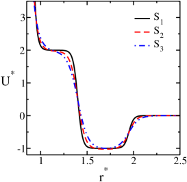
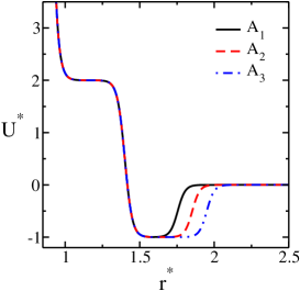
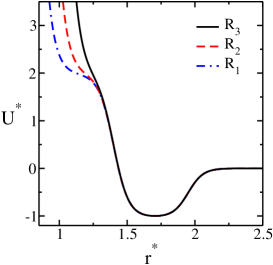
Figure 1: Interaction potential.

Table 1: Parameters for potentials $S$, $A$ and $R$ in reduced units of $\varepsilon$ and $\sigma=r_{o1}/0.950$.

Parameter	$S_{1}$	$S_{2}$	$S_{3}$	$A_{1}$	$A_{2}$	$A_{3}$	$R_{1}$	$R_{2}$	$R_{3}$
$\varepsilon^{*}_{1}$	$1.000$	$1.000$	$1.000$	$1.000$	$1.000$	$1.000$	$1.000$	$1.000$	$1.000$
$\varepsilon^{*}_{2}$	$3.000$	$3.000$	$3.000$	$3.000$	$3.000$	$3.000$	$3.000$	$3.000$	$3.000$
$-\varepsilon^{*}_{3}$	$1.000$	$1.027$	$1.023$	$1.023$	$1.023$	$1.023$	$1.023$	$1.023$	$1.023$
$r^{*}_{o1}$	$0.950$	$0.950$	$0.950$	$0.950$	$0.950$	$0.950$	$0.950$	$1.050$	$1.150$
$r^{*}_{o2}$	$1.400$	$1.400$	$1.400$	$1.400$	$1.400$	$1.400$	$1.400$	$1.400$	$1.400$
$r^{*}_{o3}$	$1.950$	$1.950$	$1.950$	$1.755$	$1.8525$	$1.950$	$1.950$	$1.950$	$1.950$
$\sigma^{*}_{1,2,3}$	$0.025$	$0.040$	$0.055$	$0.025$	$0.025$	$0.025$	$0.055$	$0.055$	$0.055$
$\alpha^{*}_{1}$	$0.000$	$0.000$	$0.000$	$0.000$	$0.000$	$0.000$	$0.000$	$0.000$	$0.000$
$\alpha^{*}_{2,3}$	$1.000$	$1.000$	$1.000$	$1.000$	$1.000$	$1.000$	$1.000$	$1.000$	$1.000$

The thermodynamic and dynamic behavior of the systems were obtained using $NVT$ molecular dynamics using Nose-Hoover heat-bath with coupling parameter $Q=2$. The system is characterized by $500$ particles in a cubic box with periodic boundary conditions, interacting with the intermolecular potential described above.

Standard periodic boundary conditions together with predictor-corrector algorithm were used to integrate the equations of motion with a time step $\Delta t^{*}=0.002$ and potential cut off radius $r_{c}^{*}=2.5$. The initial configuration is set on solid or liquid state and, in both cases, the equilibrium state was reached after $t_{eq}^{*}=1000$. From this time on the physical quantities were stored in intervals of $\Delta t_{R}^{*}=1$ during $t_{R}^{*}=1000$. The system is uncorrelated after $t_{d}^{*}=10$, from the velocity auto-correlation function, and $50$ decorrelated samples were used to get the average of the physical quantities. The thermodynamic stability of the system was checked analyzing the dependence of pressure on density, by the behavior of the energy and also by visual analysis of the final structure, searching for cavitation.

In what follows we take $\varepsilon_{1}$, $\sigma=r_{o1}/0.950$ as fundamental units for energy and distance, respectively, and all physical quantities are expressed in reduced units, namely

$$T^{*} \equiv \frac{k_{B}T}{\varepsilon_{1}}\;$$

$$\rho^{*} \equiv \rho\sigma^{3}$$

$$P^{*} \equiv \frac{P\sigma^{3}}{\varepsilon_{1}}$$

$$D^{*} \equiv \frac{D(m/\varepsilon_{1})^{1/2}}{\sigma}$$ (2)

where T, P and D are respectively temperature, pressure and diffusion coefficient. The diffusion coefficient is obtained from the expression:

$$D=\lim_{t\rightarrow\infty}\frac{\langle\left[\vec{r}_{j}(t_{0}+t)-\vec{r}_{j}(t_{0})\right]^{2}\rangle_{t_{0}}}{6t}$$ (3)

where $\vec{r}_{j}(t)$ are the coordinates of particle $j$ at time $t$, and $\langle\cdots\rangle_{t_{0}}$ denotes an average over all particles and over all $t_{0}$.

The error associated with pressure and temperature are $\Delta p^{*}\approx 0.005$ and $\Delta T^{*}\approx 0.01$.

III Results

III.1 Pressure-Temperature Phase Diagram

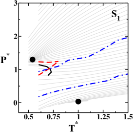
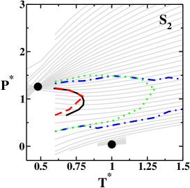
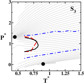
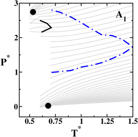
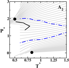
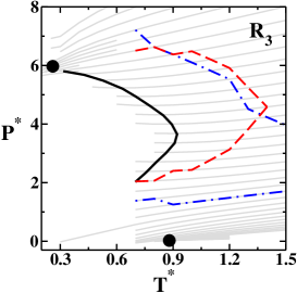
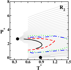
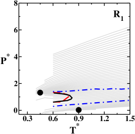
Figure 2: Pressure-temperature phase diagrams for the $S$, $A$ and $R$ families of potentials. The gray lines are isochores, the solid lines are the temperature of maximum density (TMD), the dashed lines are the extrema of diffusion and the dot-dashed line are the extrema of the translational order parameter. The filled circles are the liquid-gas (at high temperatures) and the liquid-liquid (low temperatures) critical points.

Fig. 2 presents the pressure versus temperature phase diagram obtained for the three families: $S$, $A$ and $R$. In all the nine cases the system exhibits at high temperatures a fluid phase, at intermediate temperatures and very low pressures a gas phase and at intermediate pressures a low density liquid phase (LDL) while at very high pressures a high density liquid phase (HDL). The coexistence line between the gas and the low density liquid phases (not shown) ends in a gas-LDL critical point illustrated as a filled circle in Fig. 2. The LDL-HDL coexistence line (not shown) ends in a LDL-HDL critical point also shown as a filled circle. The two critical points are located in the pressure and temperature phase diagram by the point in which the isochores meet. The critical pressures and the critical temperatures values are confirmed by analyzing the slope of the pressure versus density at constant temperature phase diagram. The maximum of these curves identify the critical point. For the other state points the slope of the pressure versus density phase diagram is also used as a check of stability.

The Table 2 and the Table 3 and the Fig 3 summarize the values of the first (liquid-gas) and second (liquid-liquid) critical points and their changes in the $p-T$ phase diagram for the three families studied.

Table 2: Liquid-gas critical point location for potentials $S$, $A$ and $R$.

Potential	$T_{c_{1}}^{*}$	$p_{c_{1}}^{*}$	Potential	$T_{c_{1}}^{*}$	$p_{c_{1}}^{*}$	Potential	$T_{c_{1}}^{*}$	$p_{c_{1}}^{*}$
$S_{1}$	$0.05$	$1.00$	$A_{1}$	$0.04$	$0.68$	$R_{1}$	$0.02$	$0.90$
$S_{2}$	$0.05$	$0.99$	$A_{2}$	$0.03$	$0.82$	$R_{2}$	$0.04$	$0.88$
$S_{3}$	$0.04$	$0.88$	$A_{3}$	$0.05$	$0.90$	$R_{3}$	$0.04$	$0.88$

Table 3: Liquid-liquid critical point location for potentials $S$, $A$ and $R$.

Potential	$T_{c_{2}}^{*}$	$p_{c_{2}}^{*}$	Potential	$T_{c_{2}}^{*}$	$p_{c_{2}}^{*}$	Potential	$T_{c_{2}}^{*}$	$p_{c_{2}}^{*}$
$S_{1}$	$1.31$	$0.54$	$A_{1}$	$2.75$	$0.53$	$R_{1}$	$1.34$	$0.44$
$S_{2}$	$1.26$	$0.48$	$A_{2}$	$1.98$	$0.50$	$R_{2}$	$2.67$	$0.37$
$S_{3}$	$1.34$	$0.44$	$A_{3}$	$1.33$	$0.44$	$R_{3}$	$6.01$	$0.26$

Fig. 2 shows that in the family of potentials $S$ the values of the pressure and temperature of the liquid-gas and the liquid-liquid critical points are not sensitive to the change of slope as predicted by Yan et al. [51]. For the $A$ family, also illustrated in Fig. 2 indicates that the temperature of the liquid-gas critical point increases with the increase of the range of the attractive scale, while the temperature and the pressure of the liquid-liquid critical point decrease. This result indicates that if the attractive scale increases the high density liquid requires less pressure to be formed while the gas phases exist for higher temperatures as predicted by Skibinstky et al. [8, 52]. In the case $R$, shown as well in the Fig. 2, the liquid-liquid critical pressure decreases with the increase of the range of the repulsive scale. This result indicates that as the repulsive scale becomes broader, it requires less pressure for the high density liquid to be formed while the repulsive scale has almost no effect in the low density liquid-gas coexistence line as predicted also by Skibinstky et al. [8, 52]. A summary of the liquid-gas and liquid-liquid critical pressures and temperatures are shown on Fig. 3.

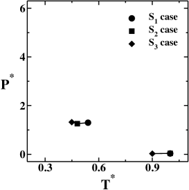
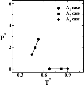
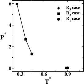
Figure 3: Location of the critical points on pressure-temperature phase diagram for cases $S$, $A$ and $R$.

III.2 Density, Diffusion and Translational Anomalies

Table 4: Limit values for density ($\rho^{*}$), temperature ($T^{*}$) and pressure ($p^{*}$) of the thermodynamics anomalies on pressure-temperature diagram. Here the point $p_{l}$ represents the density, temperature and pressure of the point of the lowest pressure in the TMD line, $p_{m}$ represents the point of the highest temperature and $p_{h}$ represents the point of the highest pressure of the TMD line.

case		$p_{l}$	$p_{m}$	$p_{h}$	case		$p_{l}$	$p_{m}$	$p_{h}$	case		$p_{l}$	$p_{m}$	$p_{h}$
	$\rho^{*}$	$0.34$	$0.35$	$0.38$		$\rho^{*}$	$0.32$	$0.34$	$0.39$		$\rho^{*}$	$0.31$	$0.34$	$0.39$
$S_{1}$	$T^{*}$	$0.70$	$0.73$	$0.60$	$S_{2}$	$T^{*}$	$0.68$	$0.80$	$0.60$	$S_{3}$	$T^{*}$	$0.60$	$0.82$	$0.61$
	$p^{*}$	$0.70$	$0.73$	$1.14$		$p^{*}$	$0.65$	$0.96$	$1.27$		$p^{*}$	$0.61$	$0.92$	$1.29$
	$\rho^{*}$	$0.42$	$0.43$	$0.45$		$\rho^{*}$	$0.37$	$0.39$	$0.42$		$\rho^{*}$	$0.31$	$0.34$	$0.39$
$A_{1}$	$T^{*}$	$0.61$	$0.71$	$0.59$	$A_{2}$	$T^{*}$	$0.51$	$0.79$	$0.69$	$A_{3}$	$T^{*}$	$0.60$	$0.82$	$0.61$
	$p^{*}$	$2.15$	$2.29$	$2.51$		$p^{*}$	$1.33$	$1.56$	$1.82$		$p^{*}$	$0.61$	$0.92$	$1.29$
	$\rho^{*}$	$0.31$	$0.34$	$0.39$		$\rho^{*}$	$0.33$	$0.37$	$0.42$		$\rho^{*}$	$0.34$	$0.39$	$0.47$
$R_{1}$	$T^{*}$	$0.60$	$0.82$	$0.61$	$R_{2}$	$T^{*}$	$0.77$	$0.92$	$0.50$	$R_{3}$	$T^{*}$	$0.70$	$0.92$	$0.32$
	$p^{*}$	$0.61$	$0.92$	$1.29$		$p^{*}$	$1.28$	$1.81$	$2.67$		$p^{*}$	$2.04$	$3.65$	$5.76$

Fig. 2 shows the temperature of maximum density (TMD) for all the nine studied cases as a solid thick lines. For all the potentials $S$, $A$ and $R$ the TMD lines are observed. The limits of the TMD in the pressure-temperature phase diagram are shown in the Table 4 where $p_{l}$ represents the values of $(\rho^{*},T^{*},p^{*})$ for the point of the lowest pressure in the TMD line, $p_{m}$ is the point with the highest temperature and $p_{h}$ is the point with the highest pressure.

The three top graphs in Fig. 2 show that the effect of decreasing the slope between the two length scales in the pair interaction potential is to move the TMD to higher temperatures. This result explains why the TMD is not observed in the discontinuous square well (DSW) model [8]. As the slope increases the TMD pressure and temperature approach the amorphous region and the system becomes unstable. For slopes higher than $S_{3}$ case no anomalous behavior is observed.

The middle graphs in Fig. 2 show that as the attractive scale increases, the TMD moves to higher temperatures and lower pressures as observed in potentials in which the attractive scale becomes dominant [53].

The bottom graphs in Fig. 2 show that as the repulsive scale becomes broader, the density anomaly region in the pressure temperature phase diagram goes to lower pressures and shrinks as observed in potentials in which the repulsive scale becomes dominant [54].

In addition in all the phase diagrams it is possible to observe that the TMD maximum pressure never exceeds the critical pressure [55]. Our results indicate that the location in the pressure temperature phase diagram of the density anomalous region depends on the distance between the two length scales [54, 53, 52].

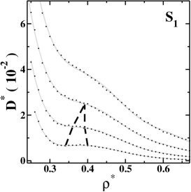
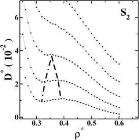
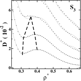
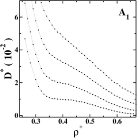
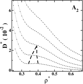
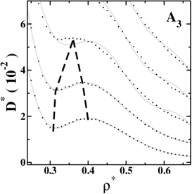
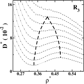
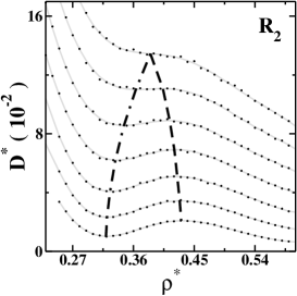
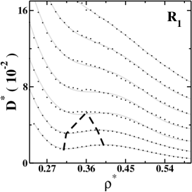
Figure 4: Diffusion coefficient as a function of density. The dots are the simulation data and the solid lines are polynomial fits. The dashed lines connect the densities of minimal and maximal diffusivity that limit the diffusion anomalous region.

The Fig. 4 shows the graphs of the dimensionless translational diffusion coefficient as function of density for all families, $S$, $A$ and $R$. The solid gray lines are a polynomial fits to the data obtained by the simulations (the dots in the Fig. 4). The diffusion coefficient follows the same trend of the TMD line. This result is not surprising since the hierarchy of the anomalies suggests that the mechanism for the presence of a TMD line is related to the mechanism for the existence of a maximum and minimum diffusion coefficient.

We also test the effects that changes in the two length scales have in the location in the pressure-temperature phase diagram of the structural anomalous region.

The translational order parameter is defined as [42, 56, 57]

$$t=\int_{0}^{\xi_{c}}\left|g(\xi)-1\right|d\xi$$ (4)

where $\xi=r\rho^{\frac{1}{3}}$ is the distance $r$ in units of the mean interparticle separation $\rho^{-\frac{1}{3}}$, $\xi_{c}$ is the cutoff distance set to half of the simulation box times [20] $\rho^{-\frac{1}{3}}$, $g(\xi)$ is the radial distribution function which is proportional to the probability of finding a particle at a distance $\xi$ from a referent particle. The translational order parameter measures how structured is the system. For an ideal gas it is $g=1$ and $t=0$, while for the crystal phase it is $g\neq 1$ over long distances resulting in a large $t$. Therefore for normal fluids $t$ increases with the increase of the density.

The graphs in Fig. 5 illustrate the translational order parameter versus density for the potentials studied. The dot-dashed lines show the maximum and minimum in the values of $t$ that limit the region of anomalous behavior. These extrema are also shown as dot-dashed lines in Figs. 2. The values at the pressure-temperature phase diagram for the different potentials follow the same trend as the TMD and diffusion anomalous regions.

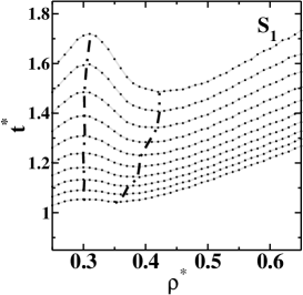
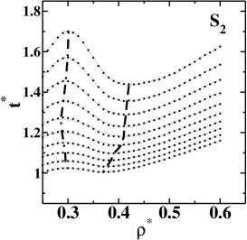
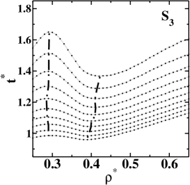
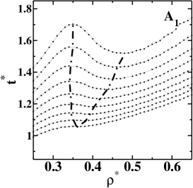
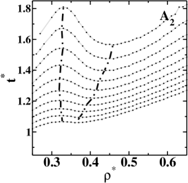
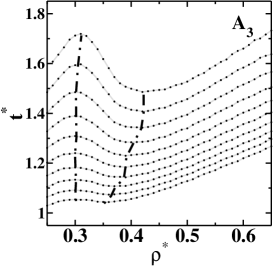
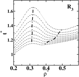
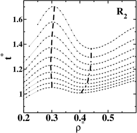
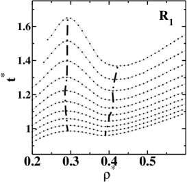
Figure 5: The translational order parameter a function of density for fixed temperatures $T^{*}=0.6,\,0.7,\,0.8,\,0.9,\,1.0,\,1.1,\,1.2,\,1.3,\,1.4,\,1.5$ (from top to bottom) for the families $S$ (on top), $A$ (on middle) and $R$ (on bottom). The dot-dashed lines locate the maximal and minimal in $t^{*}$.

III.3 Radial distribution function

The density anomaly can be related to the structure by analyzing the behavior of the radial distribution function. For a two length scales potential the $g(r)$ has two peaks: one at the closest scale, $r_{1}$, and another at the furthest scale, $r_{2}$ [20].

Recently it has been suggested that a signature of the presence of TMD line would be given by the radial distribution function as follows. At fixed temperature as the density is increased the radial distribution function of the closest scale, $g(r_{1})$, would increase its value while the radial distribution function of the furthest scale, $g(r_{2})$, would decrease. This can be represented by the rule [22, 48]

$$\Pi_{1,2}=\left.\frac{\partial g(r)}{\partial\rho}\right|_{r_{1}}\times\left.\frac{\partial g(r)}{\partial\rho}\right|_{r_{2}}<0\;\;.$$ (5)

The physical picture behind this condition [22] is that for a fixed temperature as density increases particles that are located at the attractive scale, $r_{2}$, move to the repulsive scale, $r_{1}$. Figures 6 illustrate a typical radial distribution functions for fixed $T^{*}$ as $\rho^{*}$ is varied. These graphs show that the picture of particles changing length scales due to pressure increase is valid for densities beyond a threshold density $\rho^{*}_{min}$.

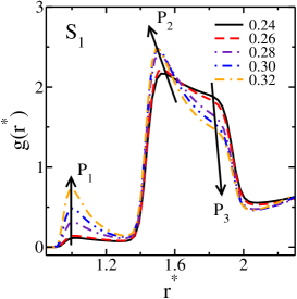
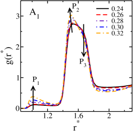
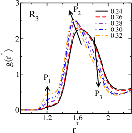
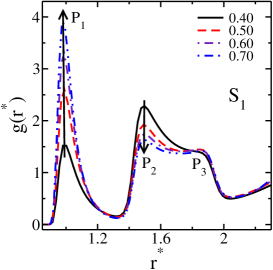
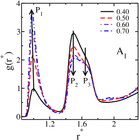
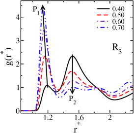
Figure 6: Radial distribution as a function of the reduced distance for selected cases in the three families of potentials for $T^{*}=0.8$. For all the families, for $\rho^{*}<0.40$ the first and second peaks of $g(r)$ increase with the increase of density. For $\rho^{*}\geq 0.40$ the first peak increases while second peak decreases with the increase of density.

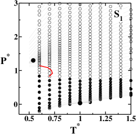
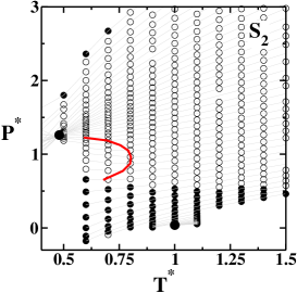
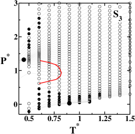
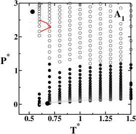
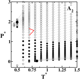
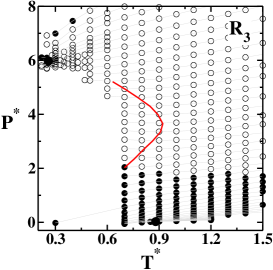
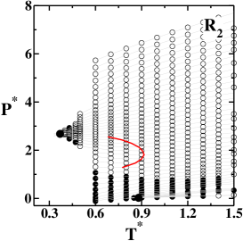
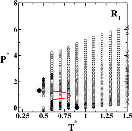
Figure 7: Pressure-temperature phase diagram for the $S$, $A$ and $R$ families of potentials, illustrating as opened circles the regions where the condition Eq. 5 is obeyed.

The regions identified by the radial distribution function as fulfilling the condition Eq. 5 are illustrated as opened circles in Fig. 7. The solid curve shows the TMD line. All the stable state points with density equal or higher the minimum density at the TMD line verify the relation $\Pi_{1,2}\left(\rho,T\right)<0$. This result gives support to our assumption that the presence of anomalies is related to particles moving from the furthest scale, $r_{2}$, to closest length scale, $r_{1}$.

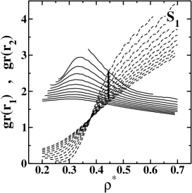
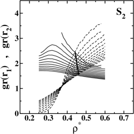
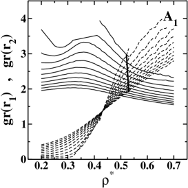
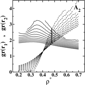
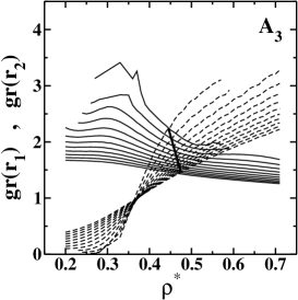
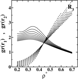
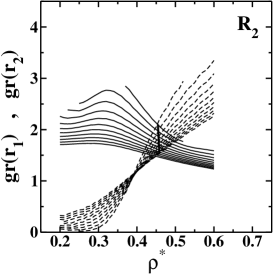
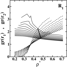
Figure 8: $g(r_{1})$ and $g(r_{2}$) for the $S$, $A$ and $R$ families of potentials as a function of the reduced density. The temperatures are $T^{*}=0.4\rightarrow 1.5$ (from top to bottom $\rho^{*}>0.6$). The solid line connects the points, for different temperatures, where $g(r_{1})=g(r_{2})$.

The Figs. 8 show the value of the radial distribution function at the closest, $g(r_{1})$ (dashed lines), and at the furthest scale, $g(r_{2})$ (solid lines), as a function of the reduced density, $\rho^{*}$. For the closest scale $g(r_{1})$ is monotonic with density while the value for the $g(r_{2})$ for a fixed temperature increases with the density for densities below the $\rho^{*}<\rho^{*}_{min}$ and decreases for densities above this threshold. This behavior, also shown in the Fig. 6, corroborates the condition stated in the Eq. 5 and supports the idea that particles move from one scale to the other by compression at $\rho>\rho_{min}$ [22].

Besides to the move of particles from the attractive scale to the repulsive scale for $\rho^{*}>\rho^{*}_{min}$ as the pressure (density) is increased, particles also move from one scale to the other due to the increase of temperature [54] for $\rho^{*}<\rho^{*}_{min}$. At constant density, $\rho^{*}<\rho^{*}_{min}$, the radial distribution function of the attractive scale, $g(r_{2})$, decreases with the increase of the temperature while $g(r_{1})$ increases with the increase of temperature, indicating that particles move from one scale to the other due to thermal effects. At the density $\rho^{*}_{min}$, the value of $g(r_{1})$ is independent of the temperature.

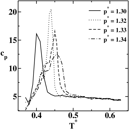
Figure 9: Isobaric specific heat for the $S_{1}$ potential for different temperatures for different pressures.

What is the meaning of the density $\rho_{min}$ in which $g(r_{1})$ is independent of temperature? As it was pointed in the previous paragraph, for $\rho^{*}<\rho^{*}_{min}$ particles move from the furthest scale, $r_{2}$, to the closest scale, $r_{1}$, using thermal energy as the temperature is increased. In this case $g(r_{1})$ increases with temperature. For $\rho^{*}>\rho^{*}_{min}$ particles move from $r_{2}$ to $r_{1}$, using the increase of pressure pressure (or density) as illustrated by the Eq. 5. From statistical point of view, the two mechanisms governing the behavior for $\rho^{*}>\rho^{*}_{min}$ and $\rho^{*}<\rho^{*}_{min}$ are quite different. While increasing temperature affects particles individually, increasing the density or the pressure affects the particles as clusters or networks. Then, as the potential becomes more soft, the threshold density $\rho^{*}_{min}$ beyond which the particles move form one scale to the other by compression should decrease as observed in Fig. 8. Therefore $\rho^{*}_{min}$ is the threshold between these two mechanisms present in systems that have density anomaly.

In addition to these low density limit, the density anomalous systems also have a high density threshold, $\rho^{*}_{max}(T)$. Fig. 8 illustrates as a solid thick line the temperatures and densities, $\rho^{*}_{max}(T)$, in which $g(r_{1})=g(r_{2})$. Since $g(r)$ is related with the number of particles at distance $r$, for $\rho^{*}<\rho^{*}_{max}(T)$ more particles are in the attractive scale, $r_{2}$, while for $\rho^{*}>\rho^{*}_{max}(T)$ more particles are at the repulsive scale $r_{1}$. Therefore, the thick solid line is a boundary between the high density liquid and the low density liquid. Analysis of the stability indicates that no real phase transition is observed across this line.

In order to understand what what happens in the region of the pressure-temperature phase diagram of the $\rho^{*}_{max}(T)$, the behavior of the specific heat in this region was analyzed. Fig. 9 shows the curves of isobaric specific heat, for different pressures as a function of the temperature for the potential $S_{1}$. The peak of $c_{p}$ for each one of the potentials analyzed in this manuscript coincide with the region $\rho^{*}_{max}(T)$ where $g(r_{1})=g(r_{2})$. This result indicates that the structure in the TMD region already build the liquid arrangements required for the liquid-liquid phase separation.

IV Conclusions

In this paper we have studied three families of core-softened potentials that exhibit two length scales, one repulsive, $r_{1}$, and another attractive, $r_{2}$.

We had observed that the region in the pressure-temperature phase diagram occupied by the TMD is quite sensitive to the slope between the two length scales. As the slope increases the region decreases. We also found that the region in the pressure-temperature phase diagram where the density, diffusion and structural anomalous behavior is observed shifts to lower pressures and shrinks the attractive scales or the repulsive scales become wider. Our results suggests the competition between two length scales are the relevant mechanism for the existence of the TMD.

In an attempt to confirm this assertion we showed in this family of potentials that the condition $\Pi_{1,2}<0$ seems to be associated with the presence of anomalous behavior. In addition we also observed that the peaks of the radial distribution function at each length scales exhibit very distinct behavior with density and temperature suggesting two complementary mechanisms for the competition between the two scales.

At low densities, $\rho^{*}<\rho^{*}_{min}$ particles move from $r_{2}$ to $r_{1}$ with the increase of temperature, using thermal energy. For densities above $\rho^{*}_{min}$ the increase of $g(r_{1})$ is associated with the increase in the pressure (density). In this interval of densities at a certain density and temperature the radial distribution function at the first length scale equals the value at the second scale, namely $g(r_{1})=g(r_{2})$. This point can be identified with the Widom line.

The relation between the radial distribution function and the Widom line, believed to be the onset of the liquid-liquid phase transition give the support to the idea that the Widom line separates two structural distinct regions that are also separated by a fragile-strong transition [18].

We expect that his result will not only shade some light in the definition of what is the shape an effective core-softened would have in order to held anomalies but also would serve to reinforce the ideas of linking dynamic transitions and thermodynamic properties.

References

- [1] P. G. Debenedetti, V. S. Raghavan, and S. S. Borick. J. Phys. Chem., 95:4540, 1991.
- [2] P. C. Hemmer and G. Stell. Phys. Rev. Lett., 24:1284, 1970.
- [3] A. Scala, M. R. Sadr-Lahijany, N. Giovambattista, S. V. Buldyrev, and H. E. Stanley. J. Stat. Phys., 100:97, 2000.
- [4] S. V. Buldyrev, G. Franzese, N. Giovambattista, G. Malescio, M. R. Sadr-Lahijany, A. Scala, A. Skibinsky, and H. E. Stanley. Physica A, 304:23, 2002.
- [5] P. Camp. Phys. Rev. E, 68:061506, 2003.
- [6] P. Camp. Phys. Rev. E, 71:031507, 2005.
- [7] C. Buzano and M. Pretti. J. Chem. Phys., 119:3791, 2003.
- [8] A. Skibinsky, S. V. Buldyrev, G. Franzese, G. Malescio, and H. E. Stanley. Phys. Rev. E, 69:061206, 2005.
- [9] G. Franzese, G. Malescio, A. Skibinsky, S. V. Buldyrev, and H. E. Stanley. Phys. Rev. E, 66:051206, 2002.
- [10] A. Balladares and M. C. Barbosa. J. Phys.: Cond. Matter, 16:8811, 2004.
- [11] A. B. de Oliveira and M. C. Barbosa. J. Phys.: Cond. Matter, 17:399, 2005.
- [12] V. B. Henriques and M. C. Barbosa. Phys. Rev. E, 71:031504, 2005.
- [13] V. B. Henriques, N. Guissoni, M. A. Barbosa, M. Thielo, and M. C. Barbosa. Mol. Phys., 103:3001, 2005.
- [14] E. A. Jagla. Phase behavior of a system of particles with core collapse. Phys. Rev. E, 58:1478, Aug. 1998.
- [15] N. B. Wilding and J. E. Magee. Phase behavior and thermodynamic anomalies of core-softened fluids. Phys. Rev. E, 66:031509, Sep. 2002.
- [16] S. Maruyama, K. Wakabayashi, and M.A. Oguni. Aip Conf. Proceedings, 708:675, 2004.
- [17] R. Kurita and H. Tanaka. Science, 206:845, 2004.
- [18] L. Xu, P. Kumar, S. V. Buldyrev, S.-H. Chen, P. Poole, F. Sciortino, and H. E. Stanley. Proc. Natl. Acad. Sci. U.S.A., 102:16558, 2005.
- [19] A. B. de Oliveira, P. A. Netz, T. Colla, and M. C. Barbosa. J. Chem. Phys., 124:084505, 2006.
- [20] A. B. de Oliveira, P. A. Netz, T. Colla, and M. C. Barbosa. J. Chem. Phys., 125:124503, 2006.
- [21] A. B. de Oliveira, M. C. Barbosa, and P. A. Netz. Physica A, 386:744, 2007.
- [22] A. B. de Oliveira, P. A. Netz, and M. C. Barbosa. Euro. Phys. J. B, 64:48, 2008.
- [23] A. B. de Oliveira, G. Franzese, P. A. Netz, and M. C. Barbosa. J. Chem. Phys., 128:064901, 2008.
- [24] A. B. de Oliveira, P. A. Netz, and M. C. Barbosa. Europhys. Lett., 85:36001, 2009.
- [25] N. V. Gribova, Y. D. Fomin, D. Frenkel, and V. N. Ryzhov. Phys. Rev. E, 79:051202, 2009.
- [26] E. Lomba, N. G. Almarza, C. Martin, and C. McBride. J. Chem. Phys., 126:244510, 2007.
- [27] D. Y. Fomin, , N. V. Gribova, V. N. Ryzhov, S. M. Stishov, and D. Frenkel. J. Chem. Phys, 129:064512, 2008.
- [28] G. S. Kell. J. Chem. Eng. Data, 20:97, 1975.
- [29] C. A. Angell, E. D. Finch, and P. Bach. J. Chem. Phys., 65:3063, 1976.
- [30] T. Tsuchiya. J. Phys. Soc. Jpn., 60:227, 1991.
- [31] C. A. Angell, R. D. Bressel, M. Hemmatti, E. J. Sare, and J. C. Tucker. Phys. Chem. Chem. Phys., 2:1559, 2000.
- [32] R. Waler. Essays of natural experiments. Johnson Reprint, New York, 1964.
- [33] R. J. Speedy and C. A. Angell. Journal of Chem. Phys., 65:851, 1976.
- [34] H. Kanno and Angell C. A. Water- anomalous compressibilities to 1.9 kbar and correlation with supercooling limits. J. Chem. Phys, 70(9):4008–4016, 1979.
- [35] C. A. Angell, M. Oguni, and W. J. Sichina. J. Phys. Chem., 86:998, 1982.
- [36] E Tombari, C Ferrari, and G Salvetti. Heat capacity anomaly in a large sample of supercooled water. Chem. Phys. Lett., 300:749–751, 1999.
- [37] H. Thurn and J. Ruska. J. Non-Cryst. Solids, 22:331, 1976.
- [38] Handbook of Chemistry and Physics. CRC Press, Boca Raton, Florida, 65 ed. edition, 1984.
- [39] G. E. Sauer and L. B. Borst. Science, 158:1567, 1967.
- [40] S. J. Kennedy and J. C. Wheeler. J. Chem. Phys., 78:1523, 1983.
- [41] R. Sharma, S. N. Chakraborty, and C. Chakravarty. J. Chem. Phys., 125:204501, 2006.
- [42] M. S. Shell, P. G. Debenedetti, and A. Z. Panagiotopoulos. Phys. Rev. E, 66:011202, 2002.
- [43] P. H. Poole, M. Hemmati, and C. A. Angell. Phys. Rev. Lett., 79:2281, 1997.
- [44] S. Sastry and C. A. Angell. Nature Mater., 2:739, 2003.
- [45] P. H. Poole, F. Sciortino, U. Essmann, and H. E. Stanley. Nature (London), 360:324, 1992.
- [46] O. Mishima and H. E. Stanley. Nature (London), 396:329, 1998.
- [47] G. Franzese, G. Malescio, A. Skibinsky, S. V. Buldyrev, and H. E. Stanley. Nature (London), 409:692, 2001.
- [48] P. Vilaseca and G. Franzese. J. Chem. Phys., 133:084507, 2010.
- [49] J. Y. Abraham, S. V. Buldyrev, and N. Giovambattista. J. Phys. Chem. B, 115:14229, 2011.
- [50] G. Malescio, G. Franzese, A. Skibinsky, S. V. Buldyrev, and H. E. Stanley. Phys. Rev. E, 71:061504, 2005.
- [51] Z. Y. Yan, S. V. Buldyrev, P. Kumar, N. Giovambattista, and H. E. Stanley. Phys. Rev. E, 77:042201, 2008.
- [52] N.M. Barraz Jr., E. Salcedo, and M.C. Barbosa. J. Chem. Phys., 135:104507, 2011.
- [53] J. da Silva, E. Salcedo, A. B. Oliveira, and M. C. Barbosa. J. Phys. Chem., 133:244506, 2010.
- [54] N.M. Barraz Jr., E. Salcedo, and M.C. Barbosa. J. Chem. Phys., 131:094504, 2009.
- [55] E. Salcedo, A. B. de Oliveira, N. M. Barraz Jr., C. Chakravarty, and M. C. Barbosa. J. Chem. Phys., 135:044517, 2011.
- [56] J. R. Errington and P. G. Debenedetti. Relationship between structural order and the anomalies of liquid water. Nature (London), 409:318, Jan. 2001.
- [57] J. E. Errington, P. G. Debenedetti, and S. Torquato. J. Chem. Phys., 118:2256, 2003.