Pulsatile Viscous Flows in Elliptical Vessels and Annuli: Solution to the Inverse Problem, with Application to Blood and Cerebrospinal Fluid Flow

Abstract

We consider the fully-developed flow of an incompressible Newtonian fluid in a cylindrical vessel with elliptical cross-section (both an ellipse and the annulus between two confocal ellipses). In particular, we address an inverse problem, namely to compute the velocity field associated with a given, time-periodic flow rate. This is motivated by the fact that flow rate is the main physical quantity which can be actually measured in many practical situations. We propose a novel numerical strategy, which is nonetheless grounded on several analytical relations. The proposed method leads to the solution of some simple ordinary differential systems. It holds promise to be more amenable to implementation than previous approaches, which are substantially based on the challenging computation of Mathieu functions. Some numerical results are reported, based on measured data for human blood flow in the internal carotid artery, and cerebrospinal fluid (CSF) flow in the upper cervical region of the human spine. As expected, computational efficiency is the main asset of our solution: a speed-up factor over $10^{3}$ was obtained, compared to more elaborate numerical approaches.

The main goal of the present study is to provide an improved source of initial/boundary data for more ambitious numerical approaches, as well as a benchmark solution for pulsatile flows in elliptical sections with given flow rate. The proposed method can be effectively applied to bio-fluid dynamics investigations (possibly addressing key aspects of relevant diseases), to biomedical applications (including targeted drug delivery and energy harvesting for implantable devices), up to longer-term medical microrobotics applications.

1 Introduction

Pulsatile flows, here intended as flows driven by a time-periodic force (generally the pressure gradient), are encountered in many contexts of practical interest. Amongst them, a remarkable case is that of heart-beat driven, human physiological flows, including blood circulation [50] and (less directly) cerebrospinal fluid (CSF) flow [31, 57]. Besides bio-fluid dynamics, time-periodic flows are widely studied with regard to e.g. chemical-physics applications, like species separation [30], as well as for mass and heat transfer problems [33, 58]. Furthermore, many studies can be found in the literature which address pulsatile flows in a more general (yet still application-driven) fluidic context, like peristaltic pumping [46], to name but one. However, in many cases of practical interest the pressure gradient is unknown or hardly measurable, and the only available datum is the time-dependent flux (hereafter, flux and flow rate are understood as synonyms). This is the most common measurement, for instance, in clinical settings regarding blood and CSF flow.

As for blood flow, it is difficult for many portions of the vasculature to keep an ideal, circular cross-section, due to the presence of surrounding organs (possibly activated by relevant muscles, or simply displaced by postural changes). Hence, while keeping some degree of abstractness, it is more appropriate to consider an elliptical cross-section to obtain a more accurate description of the flow (see e.g. [26]). As for CSF flow, the spinal sub-arachnoid space can be well approximated by an elliptical annulus [31]; CSF dynamics in such a domain is affected by pulsatility (mainly towards the upper cervical region) and plays a major role in the (still poorly understood) pathophysiology of many high-impact disease, like syringomyelia and Chiari malformation [15, 38]. Of course, in order to tackle realistic 3D flow conditions, for instance associated with patient-specific geometries, a fully numerical approach is mandatory (see e.g. [13, 28, 36, 37, 52] for the CSF case). This implies the exploitation of rather time-consuming approaches, even when adopting a classical Newtonian behavior for the working fluid (as surely appropriate for CSF [37], as well as for blood in large vessels [17, 48]). Nevertheless, it is possible to keep some degree of physical representativeness also by adopting the hypothesis of a fully-developed flow (see e.g. [24]), despite its inherent oversimplifications from a physical viewpoint. Such a position has been systematically adopted in many studies in order to obtain analytical flow solutions (see below), otherwise hardly achievable. However, even by considering a fully-developed flow, it is necessary to solve a non-standard, inverse problem in order to evaluate the velocity field (and the pressure gradient) by starting from a given flux across any cross-section of a vessel.

With reference to the above observations, we point out to expressly confine our attention to a special class of flow solutions, namely fully-developed flows of an incompressible Newtonian fluid in a straight cylinder with elliptical cross-section (either simply connected or not, see below). In particular, these assumptions permit to address a simplified linear problem, for which superposition principle holds. Nevertheless, the adopted positions aim at obtaining a benchmark solution for the inverse problem described below: this is the main target of the present work. More precisely, by virtue of the fully-developed flow hypothesis, we provide a numerical strategy which is substantially grounded on analytical relations, while being more amenable to implementation than previous ones proposed in literature. Hence, while laying no claims of generality (not even deliberately addressing realistic three-dimensional flows, e.g. within patient specific geometries and possibly involving complex rheological effects), the method we propose is credited to hold some value for obtaining at least an approximation to real flow conditions, while containing the computational cost, in the spirit of benchmark flow solutions. Furthermore, the obtained solution strategy can be used as an improved source of boundary data for more ambitious numerical approaches based on realistic data, up to serving as a debugging tool. It is worth stressing once again that we address the inverse problem, for which no straightforward approaches have been well established so far.

To better define the problem, we consider the motion of an incompressible (the constant density is here normalized to 1), Newtonian fluid in a semi-infinite straight pipe $P=E\times\mathbf{R}^{+}\subset\mathbf{R}^{3}$. In the sequel $E\subset\mathbf{R}^{2}$ will be either an ellipse or an elliptical annulus (even if results for circular cross-sections are also recalled, and some abstract results can be obtained for any smooth and bounded cross-section). The governing equations are therefore the incompressible Navier-Stokes equations which, in a reference frame with $z$ directed along the pipe axis (and $x:=(x_{1},x_{2})$ belonging to an orthogonal plane), read

$$\partial_{t}\vec{u}+(\vec{u}\cdot\nabla)\,\vec{u}-\nu\Delta\vec{u}+\nabla p=0 \qquad(x,z)\in E\times\mathbf{R}^{+},\;t\in\mathbf{R}^{+},$$

$$\nabla\cdot\vec{u}=0 \qquad(x,z)\in E\times\mathbf{R}^{+},\;t\in\mathbf{R}^{+},$$

$$\vec{u}=0 \qquad(x,z)\in\partial E\times\mathbf{R}^{+},\;t\in\mathbf{R}^{+},$$

where $\vec{u}(t,x,z)$ and $p(t,x,z)$ respectively denote velocity and pressure, and $\nu$ represents kinematic viscosity. Furthermore, as anticipated, we deliberately neglect turbulent effects by looking for a special class of solutions, namely fully-developed solutions (also named Poiseuille-type solutions) of the following form:

$$\vec{u}(t,x,z)=(0,0,w(t,x))\qquad\text{and}\qquad p(t,x,z)=-\lambda(t,x,z)+p_{0}(t),$$

where $p_{0}(t)$ denotes an arbitrary function which disappears from the equations, since pressure only enters through its spatial gradient in the formulation of the problem. In addition, the following flux condition is assumed to be satisfied:

$$\int_{E}w(t,x)\,dx=f(t),$$

for some given scalar function $f(t)$, only depending on the time variable. By standard arguments, the above Poiseuille-type ansatz implies that we may assume that the pressure has the form $p(t,z)=-\lambda(t)\,z$. Moreover, the dependence of $w$ on the space variables $x_{1}$ and $x_{2}$ allows us to consider a problem reduced to the cross-section $E$, with the given flux condition. This implies that we have to study the following problem: Find $(w(t,x),\lambda(t))$ such that

(1) $$\begin{cases}\partial_{t}w(t,x)-\nu\Delta_{x}w(t,x)=\lambda(t),&\qquad x\in E,\;t\in\mathbf{R}^{+},\\ w(t,x)=0&\qquad x\in\partial E,\;t\in\mathbf{R}^{+},\\ \int_{E}w(t,x)\,dx=f(t)&\qquad t\in\mathbf{R}^{+},\end{cases}$$

where $\Delta_{x}$ denotes the Laplacian with respect to the variables $x_{1}$ and $x_{2}$. This can be considered as an inverse problem since, if the axial pressure gradient $\lambda$ is known, one can evaluate $w$ (by solving a two-dimensional scalar heat equation) and thus the corresponding flux as well. Contrarily, in our problem the datum is the flux $f(t)$ and one wants to find the corresponding velocity and pressure associated with the fully-developed solution (such a problem is linked to one of the nowadays classical Leray’s problems [20]). For the sake of completeness, we recall that existence and uniqueness of the fully-developed solution in pipes with very general cross-sections (and with explicit but not exact expression in terms of the flux) have been recently obtained in [5, 7, 43], under reasonable regularity on the periodic $f(t)$.

The relevance of the cross-section shape on the solution process deserves some discussion at this stage. Indeed, when considering a circular cross-section, one can write an explicit solution in terms of special functions. In particular, the analytical solution of the direct problem was firstly obtained by Sexl [51] and Womersley [59] in terms of Bessel functions, while we recently derived in [6] an analytical solution to the inverse problem involving regularized confluent hyper-geometric functions. Such a fully analytical approach is made possible by the particularly simple expression taken by the Laplace operator in cylindrical coordinates. In fact, when considering an elliptical cross-section, in spite of the apparent similarity with the circular case, the situation drastically changes: an explicit solution can only be obtained for the stationary problem, while it is necessary to resort to numerical computations already when addressing the direct time-dependent problem [26, 32, 47, 55, 56]. In particular, current solutions in literature are based on involved tools like the Mathieu functions [40]. Nevertheless, some numerical approaches which also tackle the inverse problem have been recently proposed [24], still by invoking the Mathieu functions, also involving the determination of the Laplacian eigenvalues in an elliptical domain. Yet this is not a trivial task: there are several works emphasizing how instabilities can arise in the numerical computations when addressing such a problem by directly managing the Mathieu functions, especially when the ellipse eccentricity is small [26]. Indeed, computing the Mathieu functions has been recognized as the most critical issue in [24]; major efforts have been spent in order to define a wise algorithm for their evaluation.

In the light of these points, we propose an alternative numerical approach to the inverse problem of a pulsatile fully-developed flow in elliptical vessels. Our approach only indirectly addresses the Mathieu problem and therefore it does not suffer from the aforementioned limitations. Some numerical simulations are also reported, based on flow rates actually measured for human blood flow in the internal carotid artery, and CSF flow in the upper cervical region of the human spine. Corresponding results support the effective usability of our formulation (successfully coping with small eccentricities as well), by virtue of the dramatic reduction in computational time it allows, as compared to more elaborated finite element approaches. This, in turn, broadens the application spectrum of our solution, as highlighted in the last section of the present work.

Plan of the paper: In Section 2 we review relevant issues regarding stationary, fully-developed flows in elliptical cross-sections, either simply connected or not. Some results related to circular cross-sections are also recalled, for completeness. In Section 3 we propose a novel, computationally-efficient numerical strategy for solving the inverse time-dependent problem, by also exploiting an auxiliary, direct formulation. In particular, besides recalling recent results for the the circular cross-section, we discuss in detail the case of the simply connected elliptical section (being the annular case very similar). Furthermore, exemplificative numerical simulations are reported in Section 4, based on blood and CSF physiological flow data; computational cost of the proposed strategy is also compared to more elaborate, finite element numerical approaches. Concluding remarks are finally reported in Section 5, where the potential for effective application of our solution is highlighted, with explicit references to the biomedical and microrobotic research field.

2 Stationary problem

Despite being classical, the stationary solution in the elliptical cross-section is re-derived in a way that is functional to subsequent treatment. Classical results for the circular cross-section are recalled as well, for completeness. Such a stationary problem is formulated as a Poisson problem with Dirichlet boundary conditions (besides the flux condition), namely: Find $(w(x),\lambda)$ such that

(2) $$\begin{cases}-\nu\Delta_{x}w(x)=\lambda,&\qquad x\in E,\\ w(x)=0,&\qquad x\in\partial E,\\ \int_{E}w(x)\,dx=f,&\end{cases}$$

where $f\in\mathbf{R}$ is the given flux, while $\left(-\lambda\right)\in\mathbf{R}$ is the constant pressure gradient.

2.1 Stationary flow in a circular cross-section

The history of this problem dates back to the work of Hagen and Poiseuille (see e.g. [20] for details), who firstly derived the solution in a circular domain. Nonetheless, the interest for such a special solution (which can be easily derived thanks to complete separation of variables) is still considerable, as a benchmark flow also in applications to turbulence (see e.g. [44]), or for innovative biomedical applications (like magnetic particle targeting [27]). This is mainly due to the fact that Poiseuille flow represents one of the few examples of exact solution of fluid equations which are not space-periodic, yet with Dirichlet boundary conditions.

2.1.1 Flow in the circle

Let $E$ be a circle with radius $R>0$ and centered at the origin, namely: $E=\left\{(x_{1},x_{2})\in\mathbf{R}^{2}:\ |x|<R\right\}$, where $|x|=\sqrt{x_{1}^{2}+x_{2}^{2}}$. For such a case the solution to (2) is easily obtained, namely the well-known parabolic profile

(3) $$w(x)=\frac{2f}{\pi R^{2}}\left(1-\frac{|x|^{2}}{R^{2}}\right).$$

2.1.2 Flow in the circular annulus

Let $E$ be a circular annulus delimited by radii $R_{1}$ and $R_{2}>R_{1}$, namely: $E:=\left\{(x_{1},x_{2})\in\mathbf{R}^{2}:\ R_{1}<|x|<R_{2}\right\}$. In this case the solution of the Poisson problem (2) is

(4) $$w(x)=\frac{2f}{\pi\,R_{2}^{2}}\frac{\left(1-\frac{|x|^{2}}{R_{2}^{2}}\right)-\left(1-\frac{R_{1}^{2}}{R_{2}^{2}}\right)\frac{\log\left(\frac{|x|}{R_{2}}\right)}{\log\left(\frac{R_{1}}{R_{2}}\right)}}{\left(1-\frac{R_{1}^{4}}{R_{2}^{4}}\right)+\left(1-\frac{R_{1}^{2}}{R_{2}^{2}}\right)^{2}\frac{1}{\log\left(\frac{R_{1}}{R_{2}}\right)}}.$$

Notice the limiting behavior of (4) for $R_{2}=R$ and $R_{1}\to 0$.

2.2 Stationary flow in an elliptical cross-section

We review some well-known results, which will be needed later on to handle the time-dependent case. Relevant solutions for this problem originally appeared in the pioneering works of Khamrui [32] and Verma [56, 55] (besides earlier, preliminary contributions cited therein). Also in the present case it is possible to obtain an analytical solution, thanks to the particularly simple expression of the external force in the Poisson problem (2). Nonetheless, it is worth mentioning that numerical approximation of the aforementioned problem in an elliptical domain, yet with more general external forces, is the subject of ongoing research (see e.g. [35]).

2.2.1 Flow in the ellipse

Let $E=\left\{(x_{1},x_{2})\in\mathbf{R}^{2}:x^{2}_{1}/\alpha^{2}+x^{2}_{2}/\beta^{2}<1\right\}$ denote an ellipse, where $\alpha=a\cosh(b)$ and $\beta=a\sinh(b)$ respectively denote the length of the major ($x_{1}$-direction) and minor semi-axis ($x_{2}$-direction), while $2a$ represents the inter-focal distance. We preliminarily observe that the equality

(5) $$\cosh^{-1}\left(\frac{\alpha}{a}\right)=b=\sinh^{-1}\left(\frac{\beta}{a}\right)$$

implies $\log\left(\alpha/a+\sqrt{\alpha^{2}-a^{2}}/a\right)=\log\left(\beta/a+\sqrt{\beta^{2}+a^{2}}/a\right)$, from which $b=\log\left(\left(\alpha+\beta\right)/\sqrt{\alpha^{2}-\beta^{2}}\right)$ and $a=\sqrt{\alpha^{2}-\beta^{2}}$. Then, to construct the solution we introduce the natural change of variables

(6) $$\begin{cases}&x_{1}=a\cosh(\eta)\cos(\theta),\\ &x_{2}=a\sinh(\eta)\sin(\theta),\end{cases}$$

with Jacobian

(7) $$J(\eta,\theta)=a^{2}\big{[}\sinh^{2}(\eta)+\sin^{2}(\theta)\big{]}=\frac{a^{2}}{2}\left[-\frac{e^{-2i\theta}}{2}+\cosh(2\eta)-\frac{e^{2i\theta}}{2}\right].$$

By employing this change of variables we can reduce the problem in the rectangular domain

(8) $$E^{\prime}=\left\{(\eta,\theta)\in\mathbf{R}^{2}:\ 0<\eta<b\quad\text{and}\quad 0\leq\theta<2\pi\right\},$$

and it is well-known that the Laplace operator is separable with these coordinates. Furthermore, by applying the aforementioned change of variables, the Poisson equation (2) becomes

$$\left\{\begin{aligned} -\frac{\nu}{J(\eta,\theta)}\Bigg{(}\frac{\partial^{2}u}{\partial\eta^{2}}+\frac{\partial^{2}u}{\partial\theta^{2}}\Bigg{)}&=\lambda\qquad(\eta,\theta)\in E^{\prime},\\ u\text{ is $2\pi$-periodic in $\theta$}&\\ u(b,\theta)&=0\qquad\theta\in[0,2\pi[,\\ \int_{E^{\prime}}u(\eta,\theta)\,J(\eta,\theta)\,d\eta\,d\theta=f\end{aligned}\right.$$

where $u(\eta,\theta)$ simply represents $w(x)$ in the new variables (please also notice that $J>0$ for $\eta>0$). Moreover, we observe that an additional Neumann condition is needed at $\eta=0$, as detailed below. Due to periodicity in $\theta$, the solution can be written with the following complex Fourier series expansion with respect to $\theta$ (hereafter “hat” $\hat{\cdot}$ denotes a complex Fourier coefficient):

$$u(\eta,\theta)=\sum_{n\in\mathbf{Z}}\widehat{u}_{n}(\eta)\,e^{in\theta},\qquad\mathrm{where}\qquad\widehat{u}_{n}(\eta)=\frac{1}{2\pi}\int_{0}^{2\pi}u(\eta,\theta)\,e^{-in\theta}.$$

By virtue of linearity, we temporarily assume $\lambda=1$ and we recast the problem at hand as follows (for the function $u$ which is $2\pi$-periodic in $\theta$ and temporarily we do not assign the flux):

$$\left\{\begin{aligned} -{\nu}\Big{(}\frac{\partial^{2}u}{\partial\eta^{2}}+\frac{\partial^{2}u}{\partial\theta^{2}}\Big{)}&=J(\eta,\theta)\qquad&(\eta,\theta)\in E^{\prime},\\ u(b,\theta)&=0\qquad&\theta\in[0,2\pi[.\end{aligned}\right.$$

We then plug in the Poisson equation the Fourier series for both $u$ and $J(\eta,\theta)$, as given in (7), and we observe that, in order to have a real-valued solution, we need to impose as usual $\widehat{u}_{-n}=\overline{\widehat{u}_{n}}$ (hereafter “bar” $\bar{\cdot}$ denotes complex conjugacy). In particular, $\Im(\widehat{u}_{0})=0$ (hereafter $\Re$ and $\Im$ respectively denote the real and imaginary part). Moreover, by using the symmetries of the solution (reflections over the ellipse axes of symmetry) it follows that $\widehat{u}_{n}=0$ for $n$ odd. Furthermore, in order to have a smooth solution also at $\eta=0$, we need to impose $\partial_{\eta}u(0,\theta)=0$. As a result, by exploiting the above conditions, and by observing that $J$ only possesses three non-zero modes (namely those associated with $n=-2,0,2$), we obtain the following identity:

$$-\nu\sum_{n=-2,0,2}[\widehat{u}_{n}^{\prime\prime}(\eta)-n^{2}\widehat{u}_{n}(\eta)]\,e^{in\theta}=\frac{a^{2}}{2}\left[-\frac{e^{-2i\theta}}{2}+\cosh(2\eta)-\frac{e^{2i\theta}}{2}\right],$$

which corresponds to a system of three complex ordinary differential equations. In the above expression and in the sequel, “prime” $({\,\cdot\,}^{\prime})$ denotes derivative with respect to $\eta$. Then, by equating the terms corresponding to the same exponential, and by recalling the conditions at $\eta=0,b$ coming from the Dirichlet condition and from the symmetries of the solution, we have to solve the following boundary value problems:

$$\left\{\begin{aligned} &\widehat{u}_{\pm 2}^{\prime\prime}(\eta)-4\widehat{u}_{\pm 2}=\frac{a^{2}}{4\nu},\\ &\widehat{u}_{\pm 2}(b)=\Re(\widehat{u}_{\pm 2}^{\prime}(0))=\Im(\widehat{u}_{\pm 2}(0))=0,\end{aligned}\right.\qquad\text{and}\qquad\left\{\begin{aligned} &\widehat{u}_{0}^{\prime\prime}(\eta)=-\frac{a^{2}}{2\nu}\cosh(2\eta),\\ &\widehat{u}_{0}(b)=\widehat{u}_{0}^{\prime}(0)=0.\end{aligned}\right.$$

Hence, by explicitly solving these uncoupled linear differential equations we get

$$\widehat{u}_{0}(\eta)=-\frac{a^{2}}{8\nu}\left(\cosh(2\eta)-\cosh(2b)\right),\qquad\widehat{u}_{\pm 2}(\eta)=-\frac{a^{2}}{16\nu}\frac{1+e^{4b}-e^{2b-2\eta}-e^{2b+2\eta}}{1+e^{4b}}.$$

Then, by summing-up the solutions after multiplication by the corresponding complex exponential, and after some algebraic manipulations, the solution to the problem with $\lambda=1$ turns out to be

$$u(\eta,\theta)=\frac{a^{2}}{8\nu}\left(\cosh(2b)-\cos(2\theta)\right)\,\left(\cosh(2b)-\cosh(2\eta)\right)\,\text{sech}(2b),$$

being the corresponding flux

$$\int_{E^{\prime}}u(\eta,\theta)\,J(\eta,\theta)\,d\eta\,d\theta=a^{2}\,\int_{0}^{b}\left(\int_{0}^{2\pi}u(\eta,\theta)\,[\sinh^{2}(\eta)+\sin^{2}(\theta)]\,d\theta\right)\,d\eta=\frac{\pi a^{4}}{32\nu}\,\sinh^{2}(2b)\,\tanh(2b).$$

That said, the solution to the original problem (2) with given flux $f$ is finally obtained as $\left(\lambda u(\eta,\theta),\lambda\right)$, i.e. by scaling the function $u(\eta,\theta)$ computed right above by the following factor:

(9) $$\lambda=f\,\frac{{32\nu}}{\pi a^{4}}\left[\sinh^{2}(2b)\,\tanh(2b)\right]^{-1},$$

accounting for the actual flow rate. Finally, by mapping back to Cartesian coordinates, the sought solution reads

(10) $$w(x_{1},x_{2})=\frac{2f}{\pi\alpha\beta}\left[1-\frac{x^{2}_{1}}{\alpha^{2}}-\frac{x_{2}^{2}}{\beta^{2}}\right].$$

It is interesting to note how the solution (10) derives from Poiseuille solution (3) by a simple anisotropic scaling of the variables (as for obtaining the considered elliptical domain by starting from the unit circle). Thus, the elegant expression (10) (appearing in e.g. [26], yet missing in many related works) could have been obtained through simpler derivations. Nevertheless, we deliberately decided to introduce many details above, since they serve as useful references for the solution of the corresponding time-dependent problem. On regard, it should be noticed how, despite separation of variables (in elliptical coordinates), ellipticity per se creates a new situation already when considering stationary conditions: there appear 3 coupled modes in the solution (contrarily to the fully decoupled flow solution in the circle). Such a difference persists and it is somehow magnified in the time-dependent case, where more complex behaviors naturally appear (see Section 3).

2.2.2 Flow in the elliptical annulus

Given the inter-focal distance $2a$, it is straightforward to apply (6) in order to also map two confocal ellipses into a rectangular region. More precisely, given semi-axes $\alpha_{1},\beta_{1}$ and $\alpha_{2},\beta_{2}$, with $\beta_{2}>\beta_{1}$, the rectangle $E^{\prime}=\left\{(\eta,\theta)\in\mathbf{R}^{2}:\ b_{1}<\eta<b_{2}\quad\text{and}\quad 0\leq\theta<2\pi\right\}$ is obtained, where $b_{1}$ and $b_{2}>b_{1}$ are derived from the respective semi-axes through (5). For this problem we have Dirichlet boundary conditions at both $\eta=b_{1}$ and $\eta=b_{2}$. Hence, by enforcing the symmetries $\widehat{u}_{-n}=\overline{\widehat{u}_{n}}$ needed to have real-valued velocities, we end up with the following boundary value problems (for the auxiliary problem with $\lambda=1$):

$$\left\{\begin{aligned} &\widehat{u}_{\pm 2}^{\prime\prime}(\eta)-4\widehat{u}_{\pm 2}=\frac{a^{2}}{4\nu},\\ &\widehat{u}_{\pm 2}(b_{1})=\widehat{u}_{\pm 2}(b_{2})=0,\end{aligned}\right.\qquad\text{and}\qquad\left\{\begin{aligned} &\widehat{u}_{0}^{\prime\prime}(\eta)=-\frac{a^{2}}{2\nu}\cosh(2\eta)\\ &\widehat{u}_{0}(b_{1})=\widehat{u}_{0}(b_{2})=0,\end{aligned}\right.$$

whose solutions, by direct integration, read:

$$\widehat{u}_{0}(\eta) = \frac{a^{2}}{8\nu}\left[\frac{(\eta-b_{1})\cosh(2b_{2})-(\eta-b_{2})\cosh(2b_{1})}{(b_{2}-b_{1})}-\cosh(2\eta)\right],$$

$$\widehat{u}_{\pm 2}(\eta) = \frac{a^{2}}{16\nu}\left[\frac{e^{2(\eta-b_{2})}-e^{-2(\eta-b_{2})}-e^{2(\eta-b_{1})}+e^{-2(\eta-b_{1})}}{e^{2(b_{1}-b_{2})}-e^{-2(b_{1}-b_{2})}}-1\right],$$

so that the following stationary solution for the auxiliary problem is obtained (cf. [55]):

$$u(\eta,\theta) = \frac{a^{2}}{8\nu}\left[\frac{(\eta-b_{1})\cosh(2b_{2})-(\eta-b_{2})\cosh(2b_{1})}{(b_{2}-b_{1})}\;+\right.$$

$$\qquad\quad\left.\frac{\sinh(2(\eta-b_{1}))-\sinh(2(\eta-b_{2}))}{\sinh(b_{2}-b_{1})}\cos(2\theta)-(\cosh(2\eta)+\cos(2\theta))\right].$$

Finally, by reasoning as in Section 2.2.1, the solution to (2) with given flux $f$ is obtained as $\left(\lambda u(\eta,\theta),\lambda\right)$, with (cf. [24])

$$\lambda=f\,\frac{16\nu}{\pi a^{4}}\left[\frac{(\sinh(4b_{2})-\sinh(4b_{1}))}{4}-\frac{(\cosh(2b_{2})-\cosh(2b_{1}))^{2}}{2(b_{2}-b_{1})}-\frac{\cosh(2(b_{2}-b_{1}))-1}{\sinh(2(b_{2}-b_{1}))}\right]^{-1}.$$

Following [55], it is worth remarking that the solution in the (simply connected) ellipse cannot be obtained as a limit case of the one in the annulus, due to the constraint of confocality. Indeed, by allowing $b_{1}\to 0$, the inner boundary of the annulus (where the Dirichlet condition also applies) degenerates to the inter-focal segment. The resulting flow field is therefore that one associated with an ellipse with semi-axes $\alpha_{2}$ and $\beta_{2}$, yet also containing a plate having width equal to the inter-focal distance $2a$.

3 Time-dependent problem

We now address the time-periodic elliptical case, by proposing a novel numerical method for its solution (this is the main asset of the present study). More in detail, we firstly recall the solution of the inverse problem for the flow in the circle, so as to keep some degree of symmetry with Section 2. We then address the elliptical case, where we solve the inverse problem by exploiting relevant results, purposely introduced through an auxiliary, direct formulation. In particular, we accurately report the solution method for the simply connected elliptical cross-section. Conversely, we omit details for the flow in the elliptical annulus between two confocal ellipses, since it can be derived from the previous case by a straightforward modification of the boundary conditions, as mentioned in Section 2.2.2; corresponding numerical results are nonetheless reported in Section 4.2, for the sake of completeness.

3.1 Flow in the circle: the inverse problem

Let us preliminarily introduce the following $T$-periodic functions:

(11) $$\lambda(t)=\sum_{m\in\mathbf{Z}}\widehat{\lambda}_{m}e^{i\omega_{m}t},\quad f(t)=\sum_{m\in\mathbf{Z}}\widehat{f}_{m}e^{i\omega_{m}t},\quad w(x,t)=\sum_{m\in\mathbf{Z}}\widehat{w}_{m}(x)\,e^{i\omega_{m}t},\quad\quad\omega_{m}=\frac{2\pi m}{T}.$$

The aforementioned works by Sexl [51] and Womersley [59] addressed the direct problem, that is with assigned pressure gradient $\lambda(t)$. Corresponding solution can be constructed as an infinite series of Bessel functions $J_{0}$ of order zero (Womersley considered a single Fourier mode, yet superposition can be invoked under the assumptions in [5], since the corresponding sequence formally converges). As regards the inverse problem, an explicit map between the Fourier coefficients of the velocity $\widehat{w}_{m}$ and those of the flow rate $\widehat{f}_{m}$ has been recently obtained by the authors [6]. Relevant relations read

$$\widehat{f}_{m}=\pi R^{2}\,\left(1-\frac{\,{}_{0}\tilde{F}_{1}\left(;2;i\,\mathrm{Wo}^{2}_{R,m}\,/4\right)}{\,{}_{0}\tilde{F}_{1}\left(;1;i\,\mathrm{Wo}^{2}_{R,m}\,/4\right)}\right)\,\,\frac{\widehat{\lambda}_{m}}{i\omega_{m}},\qquad\widehat{w}_{m}=\left(1-\frac{J_{0}\left((-1)^{3/4}\,\mathrm{Wo}_{r,m}\right)}{J_{0}\left((-1)^{3/4}\,\mathrm{Wo}_{R,m}\right)}\right)\,\,\frac{\widehat{\lambda}_{m}}{i\omega_{m}},$$

where $\,{}_{0}\tilde{F}_{1}(;\cdot;\cdot)$ denotes the regularized confluent hyper-geometric function, and

(12) $$\mathrm{Wo}_{r,m}=r\,\sqrt{\frac{\omega_{m}}{\nu}},$$

is a non-dimensional parameter which generalizes the classical Womersley number.

3.2 Flow in the ellipse: the auxiliary direct problem

The explicit solution for the direct problem in an elliptical vessel was originally derived by Khamrui [32] (although some details were missing) and Verma [56], following the same approach of Womersley. In particular, given a single harmonic pressure gradient $\lambda=e^{i\omega_{m}t}$, with $m\in\mathbf{Z}$, the solution (in elliptical coordinates) is the following:

(13) $$u(\eta,\theta)=\sum_{n=0}^{\infty}C_{2n}\,\,{C\!e}_{2n}(\eta,-q)\,{ce}_{2n}(\theta,-q),\quad\mathrm{with}\quad q=\frac{i\,a^{2}\,\omega_{m}}{4\,\nu}.$$

The functions $C\!e_{2n}$ and ${ce}_{2n}$ in (13) respectively denote the ordinary and modified Mathieu functions [40], while $C_{2n}$ represent suitable constants, determined from the no-slip (i.e. Dirichlet) boundary condition. It must be remarked that, despite the aforementioned functions were originally introduced by Mathieu in the 19th century (to study the vibration of an elliptical membrane, and they are still applied in the field [12]), they still deserve attention from a computational viewpoint, since their evaluation is prone to numerical instabilities [53]. Moreover, in order to get a $\theta$-periodic solution through the Mathieu functions (as in the present case), one needs to evaluate the eigenvalues of the Laplacian: this involves infinite tridiagonal matrices and it is very expensive. Furthermore, practical limitations on the ellipticity $\epsilon=\beta/\alpha$ arise when directly using these special functions; see e.g. [26], where numerical instabilities are reported for $\epsilon<0.3$ (besides interesting expressions for $\epsilon\to 1$, that is for elliptical cross-sections degenerating to the circular geometry). In light of these points, the quest for robust numerical methods able to efficiently compute the Mathieu functions is still an open issue, and positive contributions are being provided. In particular, a stepwise procedure is proposed in [24], suitable for evaluating the Mathieu functions in correspondence to large complex arguments typically associated with viscous flows. Such a strategy exploits a proper blend of backward and forward recurrence techniques in order to enhance the convergence of the involved computations.

In order to circumvent the aforementioned limitations, we propose a novel numerical strategy, in the spirit of Fourier analysis, which only involves the Mathieu functions in an indirect way. In particular, we extend the approach introduced in [35] for the stationary case to the time-dependent one: our approach is based on a Fourier analysis in the variables $\theta$ and $t$, while the problem in the variable $\eta$ is kept in the physical space. More in detail, by applying the change of variables introduced in (6), we firstly recast the time-dependent problem as follows:

(14) $$u_{t}(t,\eta,\theta)\,J(\eta,\theta)-\nu\left(\frac{\partial^{2}u(t,\eta,\theta)}{\partial\eta^{2}}+\frac{\partial^{2}u(t,\eta,\theta)}{\partial\theta^{2}}\right)=J(\eta,\theta)\,\lambda(t).$$

Then, since we look for $T$-periodic solutions (besides needing $2\pi$-periodicity with respect to $\theta$), we make the following ansatz of separation of variables for the velocity:

(15) $$u(t,\eta,\theta)=\sum_{m,n\in\mathbf{Z}}\widehat{u}_{m,n}(\eta)\,e^{in\theta}e^{i\omega_{m}t},$$

hereafter considered in place of the corresponding one in (11). Furthermore, since we consider real-valued solutions, the following conditions immediately apply: $\widehat{\lambda}_{-m}=\overline{\widehat{\lambda}_{m}}$, $\widehat{f}_{-m}=\overline{\widehat{f}_{m}}$ and $\widehat{u}_{-m,-n}=\overline{\widehat{u}_{m,n}}$ (latter relation implies, in particular, $\Im(\widehat{u}(\eta)_{0,0})=0$).

We then start by deliberately addressing a direct problem, hence by assuming a given pressure gradient. In order to stress the fact that we temporarily turn our attention to a direct problem, we introduce a minor notation change (just within this section) by denoting the pressure gradient as $\sigma(t)=\sum_{m\in\mathbf{Z}}\widehat{\sigma}_{m}e^{i\omega_{m}t}$. By plugging (15) into (14), we arrive at the following problem: Solve, for each $m\in\mathbf{Z}$,

(16) $$\left\{\begin{aligned} \sum_{n\in\mathbf{Z}}i\,\omega_{m}\widehat{u}_{m,n}(\eta)\,e^{in\theta}J(\eta,\theta)-{\nu}\big{(}\widehat{u}_{m,n}^{\prime\prime}(\eta)-n^{2}\widehat{u}_{m,n}(\eta)\big{)}\,e^{in\theta}&=J(\eta,\theta)\,\widehat{\sigma}_{m}\\ \widehat{u}_{m,n}(b)&=0\qquad n\in\mathbf{Z},\end{aligned}\right.$$

with $(\eta,\theta)\in E^{\prime}$ and $E^{\prime}$ defined as in (8). The considered problem can be immediately simplified by invoking symmetry: velocity must be unchanged by the transformations $\theta\mapsto-\theta$ and $\theta\mapsto\pi-\theta$, i.e. by reflection over the ellipse axes of symmetry. This, by also recalling the above conditions on conjugacy, provides

(17) $$\widehat{u}_{m,n}=0\quad\text{for $n$ odd}\quad\text{and}\quad\widehat{u}_{m,-n}=\widehat{u}_{m,n},\,\,\widehat{u}_{-m,n}=\overline{\widehat{u}_{m,-n}}=\overline{\widehat{u}_{m,n}},\quad\text{for $n$ even, $m\in\mathbf{Z}$.}$$

Hence, we only need to solve the equations for the Fourier modes $\widehat{u}_{m,n}$, with $n,m\in\mathbf{Z}$ both greater or equal to zero, with $n$ even. This permits to reduce by a factor eight the computational burden. That said, by plugging into (16) the Fourier expansion of $J$ given in (7) and by equating the corresponding even $n$-modes (at fixed $m$), we obtain the following infinite family of ordinary differential equations

(18) $$\begin{array}[]{rcl}\widehat{u}^{\prime\prime}_{m,0}-\bigg{[}\frac{i\,\mathrm{Wo}^{2}_{a,m}}{2}\cosh(2\eta)\bigg{]}\,\widehat{u}_{m,0}+\frac{i\,\mathrm{Wo}^{2}_{a,m}}{2}\,\widehat{u}_{m,2}&=&-\frac{a^{2}}{2\nu}\cosh(2\eta)\,\widehat{\sigma}_{m}\\ \widehat{u}^{\prime\prime}_{m,2}-\bigg{[}2^{2}+\frac{i\,\mathrm{Wo}^{2}_{a,m}}{2}\cosh(2\eta)\bigg{]}\,\widehat{u}_{m,2}+\frac{i\,\mathrm{Wo}^{2}_{a,m}}{4}\,(\widehat{u}_{m,4}+\widehat{u}_{m,0})&=&\frac{a^{2}}{4\nu}\,\widehat{\sigma}_{m}\\ \widehat{u}^{\prime\prime}_{m,4}-\bigg{[}4^{2}+\frac{i\,\mathrm{Wo}^{2}_{a,m}}{2}\cosh(2\eta)\bigg{]}\,\widehat{u}_{m,4}+\frac{i\,\mathrm{Wo}^{2}_{a,m}}{4}\,(\widehat{u}_{m,6}+\widehat{u}_{m,2})&=&\ \ 0\\ \vdots&\vdots&\quad\vdots\\ \widehat{u}^{\prime\prime}_{m,2n}-\bigg{[}(2n)^{2}+\frac{i\,\mathrm{Wo}^{2}_{a,m}}{2}\cosh(2\eta)\bigg{]}\,\widehat{u}_{m,2n}+\frac{i\,\mathrm{Wo}^{2}_{a,m}}{4}\,(\widehat{u}_{m,2n+2}+\widehat{u}_{m,2n-2})&=&\ \ 0\\ \vdots&\vdots&\quad\vdots\end{array}$$

where we use $\widehat{u}_{m,n}$ in place of $\widehat{u}_{m,n}(\eta)$ for brevity, and $\mathrm{Wo}_{a,m}$ is a generalized Womersley number based on the semi-focal distance $a$, defined as in (12). Please also notice that $q=i\mathrm{Wo}^{2}_{a,m}/4$, with $q$ introduced in (13) (cf. e.g. [24, 26]). Furthermore, as in the stationary case, we need to assign an additional condition at $\eta=0$ (where the change of coordinates becomes singular) in order to have a well-posed mixed boundary value problems for $\widehat{u}_{m,n}$. In particular, for the solution to be smooth also near $\eta=0$, it is suitable to enforce symmetry for the velocity-profile, i.e. a vanishing velocity gradient normal to the inter-focal line. This reads (cf. [26, Eq. (9)]) $\partial_{\eta}u(0,\theta,t)=0$, that is $\widehat{u}^{\prime}(0)_{m,n}=0$.

The equations (18) represent an infinite system of non-homogeneous Mathieu ordinary differential equations. In order to get a computable system, one main idea is to approximate such a system with a finite dimensional (large enough) system of coupled ordinary differential equations. However, this cannot be achieved by simply neglecting all equations which involve modes $\widehat{u}_{m,n}$ for large enough $|n|$, since there is an infinite coupling (indeed, for each $n\in\mathbf{Z}$, the equation for $n$-th mode is coupled with those of the two closest modulo 2 $n$-modes, thus providing a tridiagonal system) and such a rough simplification would lead to a system without solutions. The main idea in the present study is that higher frequencies are asymptotically small, since they are terms of a convergent Fourier series. The fact that the series converges derives from the abstract results in [5, 21], which can be even simplified in the case of an assigned smooth and periodic pressure gradient. Hence, by assuming that $\widehat{f}_{m}$ vanishes fast enough as $|m|\to+\infty$ (and this is more than reasonable for realistic flows, see also Section 4), the assumed smallness of the higher modes is fully justified. Therefore, once chosen a cut-off index $N\in\mathbf{N}$ ($N\geq 2$ to keep at least the first equation having zero as right-hand-side), we neglect $\widehat{u}_{m,n}$ for all $n\in\mathbf{Z}$ such that $|n|>2N$ since, in light of the aforementioned assumption, this does not affect the solution in a significant manner. From a practical viewpoint and based on the symmetries highlighted above, this implies to drop off $\widehat{u}_{m,2N+2}$ in the differential equation satisfied by $\widehat{u}_{m,2N}$, and to only solve the equations for $\widehat{u}_{m,n}$ with $n=0,2,\ldots,2N$. In this way, for each $m\in\mathbf{N}\cup\{0\}$, we end up with a closed tridiagonal system of linear ordinary differential equations: it naturally represents the differential counterpart of the tridiagonal matrix which is obtained when evaluating the eigenvalues of the Mathieu functions by truncating the corresponding algebraic linear system (see e.g. [1, 24]).

Before stating the tridiagonal system we actually address, we remark that, by virtue of linearity, it is convenient for our purposes to directly assume $\widehat{\sigma}_{m}=1$. Moreover, we denote the unknown by $\widehat{v}_{m,n}$ in order to stress that, besides adopting a unitary pressure gradient, we are approximating $\widehat{u}_{m,n}$ by truncation. In light of the above arguments and derivations, for each $m\in\mathbf{N}\cup\{0\}$ we have to solve the following boundary value problem:

(19) $$\left\{\begin{array}[]{rcl}\widehat{v}^{\prime\prime}_{m,0}-\bigg{[}\frac{i\,\mathrm{Wo}^{2}_{a,m}}{2}\cosh(2\eta)\bigg{]}\,\widehat{v}_{m,0}+\frac{i\,\mathrm{Wo}^{2}_{a,m}}{2}\widehat{v}_{m,2}&=&-\frac{a^{2}}{2\nu}\cosh(2\eta)\\ \widehat{v}^{\prime\prime}_{m,2}-\bigg{[}2^{2}+\frac{i\,\mathrm{Wo}^{2}_{a,m}}{2}\cosh(2\eta)\bigg{]}\,\widehat{v}_{m,2}+\frac{i\,\mathrm{Wo}^{2}_{a,m}}{4}(\widehat{v}_{m,4}+\widehat{v}_{m,0})&=&\frac{a^{2}}{4\nu}\\ \widehat{v}^{\prime\prime}_{m,4}-\bigg{[}4^{2}+\frac{i\,\mathrm{Wo}^{2}_{a,m}}{2}\cosh(2\eta)\bigg{]}\,\widehat{v}_{m,4}+\frac{i\,\mathrm{Wo}^{2}_{a,m}}{4}(\widehat{v}_{m,6}+\widehat{v}_{m,2})&=&\ \ 0\\ \vdots&=&\quad\vdots\\ \widehat{v}^{\prime\prime}_{m,2n}-\bigg{[}(2n)^{2}+\frac{i\,\mathrm{Wo}^{2}_{a,m}}{2}\cosh(2\eta)\bigg{]}\,\widehat{v}_{m,2n}+\frac{i\,\mathrm{Wo}^{2}_{a,m}}{4}(\widehat{v}_{m,2n+2}+\widehat{v}_{m,2n-2})&=&\ \ 0\\ \vdots&=&\quad\vdots\\ \widehat{v}^{\prime\prime}_{m,2N-2}-\bigg{[}(2N-2)^{2}+\frac{i\,\mathrm{Wo}^{2}_{a,m}}{2}\cosh(2\eta)\bigg{]}\,\widehat{v}_{m,2N-2}+\frac{i\,\mathrm{Wo}^{2}_{a,m}}{4}(\widehat{v}_{m,2N}+\widehat{v}_{m,2N-4})&=&\ \ 0\\ \widehat{v}^{\prime\prime}_{m,2N}-\bigg{[}(2N)^{2}+\frac{i\,\mathrm{Wo}^{2}_{a,m}}{2}\cosh(2\eta)\bigg{]}\,\widehat{v}_{m,2N}+\frac{i\,\mathrm{Wo}^{2}_{a,m}}{4}(\widehat{v}_{m,2N-2})&=&\ \ 0\\ \\ \widehat{v}_{m,n}(b)=0\qquad n=0,2,\dots,2N,&&\\ \widehat{v}^{\prime}_{m,n}(0)=0\qquad n=0,2,\dots,2N.&&\end{array}\right.$$

It is worth remarking how, instead of truncating an infinite dimensional algebraic linear system in order to evaluate corresponding eigenvalues (as in [24]), we performed a Galerkin-type truncation of the system of ordinary differential equations which stems from the Fourier separation of variables. It is in this sense that we only indirectly referred to Mathieu functions, thus circumventing the numerical challenges associated therewith (indeed, we end up with a very simple tridiagonal system, which can be straightforwardly solved).

Remark 20.

An alternative pathway for solving the considered direct problem would be that of [21]: By considering real (i.e. sine and cosine) Fourier series functions, to solve the following system for the unknowns $(\phi_{m},\psi_{m})$: $-n\psi_{m}=\nu\Delta\phi_{m}+1$, $n\phi_{m}=\nu\Delta\psi_{m}$, coupled with vanishing Dirichlet conditions. Indeed, the above system can be used to prove the existence of time-periodic solutions in an abstract way. However, in view of our main objective of obtaining a benchmark solution for the flow in elliptical cross-sections, it seems less convenient to follow such a strategy, since it involves the bi-Laplacian operator, which seems not to be easily manageable by separation of variables in elliptical coordinates.

In a practical framework, it is necessary to only solve the system (19) for $m\in\mathcal{M}^{\star}$, where $\mathcal{M}^{\star}=\{0,1,\ldots,M^{\star}\}$, $M^{\star}$ denoting a sort of upper bound for the harmonic content of the given flow rate (i.e. its highest yet still relevant $t$-frequency is assumed to be $\omega_{M^{\star}}$). Moreover, once fixed the fluid (i.e. $\nu$) and the size of the cross-section (i.e. $a$ and $b$), the solution of (19) is only affected by the adopted cut-off index $N$. Let us stress this point by introducing the more descriptive notation $\widehat{v}^{(2N)}_{m,n}$, as an alternative to $\widehat{v}_{m,n}$. Hence, it is mandatory to choose $N$ large enough to get a proper approximation for all the modes $\widehat{v}^{(2N)}_{m,n}$, in particular for $m$ up to $M^{\star}$. Let us denote by $N^{\star}$ the sought value of $N$, to remind that it also depends on $M^{\star}$. Two assets can be introduced to the purpose: accuracy (magnitude of the cut modes must be negligible compared to that of the kept ones) and independence from $N$ (truncation must only affect the kept modes in a negligible way). As discussed above, higher frequencies are expected to be small than lower ones (by Fourier convergence); hence the accuracy asset can be formulated by introducing the following non-dimensional quantity:

(21) $$\mu(m,N)=\frac{\|\widehat{v}_{m,2N}^{(2N)}\|_{\infty}}{\|\widehat{v}_{m,0}^{(2N)}\|_{\infty}},$$

where $\|\widehat{v}\|_{\infty}=\max_{\eta\in E^{\prime}_{\eta}}|\widehat{v}(\eta)|$, $E^{\prime}_{\eta}=[0,b]$ denotes the considered $\eta$-range, and the $n=0$ mode is used to get a reference value. (Such a reference was used for the numerical tests in Section 4, turning out to be non-vanishing; otherwise, alternative choices can be introduced by exploiting larger $n$ values.) In particular, once chosen a threshold $\bar{\mu}$, let us define an index $N^{\star}_{\bar{\mu}}$ as the smallest integer $N$ such that $\mu(m,N)\leq\bar{\mu}$, for all $m\in\mathcal{M}^{\star}$. Hence, by choosing $N\geq N^{\star}_{\bar{\mu}}$ we are guaranteed that truncation only cuts negligible $n$-modes, for all relevant values of $m$. As regards independence from $N$, the following non-dimensional quantity is introduced:

(22) $$s(m,N)=\displaystyle\max_{n\in\mathcal{N}}\frac{\|\widehat{v}_{m,n}^{(2N)}-\widehat{v}_{m,n}^{(2N+2)}\|_{\infty}}{\|\widehat{v}_{m,0}^{(2N)}\|_{\infty}},$$

where $\mathcal{N}=\{0,2,\dots,2N-2\}$ (index $N$ is not considered, for obvious reasons). Then, once chosen a threshold $\bar{s}$, let us define an index $N^{\star}_{\bar{s}}$ as the smallest integer $N$ such that $s(m,N)\leq\bar{s}$, for all $m\in\mathcal{M}^{\star}$. Hence, by choosing $N\geq N^{\star}_{\bar{s}}$ we are guaranteed that truncation only negligibly affects the kept $n$-modes, for all relevant values of $m$. Finally, we naturally define $N^{\star}=\max\left(N^{\star}_{\bar{\mu}},N^{\star}_{\bar{s}}\right)$, so as to achieve both targeted assets.

3.3 Flow in the ellipse: the inverse problem

The interest in a benchmark solution for the inverse problem in elliptical cross-sections has been highlighted in Section 1. Nevertheless, some relevant results have been only recently provided in [24], grounded on the solution of the direct problem by direct computation of the Mathieu functions, as discussed in Section 3.2 (earlier attempts in [49] seem to be loosely grounded on a theoretical basis). In order to circumvent the aforementioned challenges related to such a computation, we propose an alternative method which is based on the fast-Fourier approach introduced in Section 3.2. Thanks to linearity, we simply need to link the Fourier coefficients of the flow rate with those of the pressure gradient (as in the stationary case, thus generalizing (9)). The relevant solution strategy is described below.

The flow rate associated with the ansatz (15) reads

$$f(t)=\sum_{m\in\mathbf{Z}}\widehat{f}_{m}\,e^{i\omega_{m}t}=\sum_{m\in\mathbf{Z}}\left[\,\sum_{n\in\mathbf{Z}}\int_{0}^{b}\widehat{u}_{m,n}(\eta)\left(\int_{0}^{2\pi}e^{in\theta}\,J(\eta,\theta)\,d\theta\right)d\eta\right]\,e^{i\omega_{m}t}.$$

Then, once substituted $J$ from (7), by explicit calculations we get

$$\frac{1}{a^{2}}\int_{0}^{2\pi}e^{in\theta}\,J(\eta,\theta)\,d\theta=\left\{\begin{aligned} &-\pi/2&n=\pm 2,\\ &\pi\cosh(2\eta)&n=0,\\ &0&n\in\mathbf{Z}\backslash\{0,\pm 2\},\end{aligned}\right.$$

so that the following relation can be easily obtained, for each $m\in\mathbf{Z}$:

(23) $$\widehat{f}_{m}=\frac{a^{2}\pi}{2}\int_{0}^{b}\Big{(}-\widehat{u}_{m,-2}(\eta)+2\cosh(2\eta)\,\widehat{u}_{m,0}(\eta)-\widehat{u}_{m,2}(\eta)\Big{)}\,d\eta.$$

Clearly, without an explicit knowledge of $\widehat{u}_{m,n}(\eta)$ (i.e. of the sought solution), it is not possible to evaluate the flux by means of (23). Nevertheless, by recalling from Section 3.2 the approximate solution $\widehat{v}_{m,n}$ (associated with a unitary pressure gradient), it is straightforward to exploit (23) in order to approximate the Fourier coefficients $\widehat{\lambda}_{m}$ (of the unknown pressure gradient) in terms of $\widehat{f}_{m}$. Indeed, thanks to linearity and by also recalling (17), the following relation is immediately obtained, for each $m\in\mathbf{N}\cup\{0\}$:

(24) $$\widehat{\lambda}_{m}\cong\widehat{f}_{m}\,\frac{1}{\pi a^{2}}\left[\int_{0}^{b}\big{(}\cosh(2\eta)\,\widehat{v}_{m,0}(\eta)-\widehat{v}_{m,2}(\eta)\big{)}\,d\eta\right]^{-1}.$$

Latter expression deserves a remark: the bracketed quantity must be non-vanishing for such an expression to be meaningful. If we consider the exact solution $\widehat{u}_{m,n}$ of the infinite dimensional system (based on explicit knowledge of the asymptotic behavior of appropriate Hilbertian norms of eigenfunctions of the bi-Laplace operator in the domain under consideration, as for the existence results proved in [5, 21]), then the map between $\widehat{f}_{m}$ and $\widehat{\lambda}_{m}$ is one-to-one. This, in turn, implies a non-vanishing denominator in the expression corresponding to (24). Yet such a condition is not perfectly guaranteed when considering an approximate solution $\widehat{v}_{m,n}$. Nonetheless, if the numerical approximation is accurate enough (i.e. for a cut-off index $N$ large enough), the approximate denominator is close enough to the exact one for the non-vanishing condition to be fulfilled. It must be pointed out that the same potentially critical issue occurs when directly using the Mathieu functions. For instance, in [24] the authors implicitly rely on a well-defined mapping between flow rate and pressure coefficients for obtaining their solution. In that case, the degree of the involved Mathieu functions must be large enough for the associated numerical method to be well-posed, in complete analogy with the present case.

Having introduced the main ingredients, it is now possible to summarize the basic steps we propose for solving the inverse problem:

• We start by choosing a fluid (thus the kinematic viscosity $\nu$) and the size (namely $a$ and $b$) of the considered vessel cross-section. We also assume a given flow rate $f(t)$ having period $T$;

• We determine an integer $M$ such that the Fourier spectrum of $f(t)$ is suitably approximated by considering $M$ modes; popular metrics (e.g. the Pearson correlation coefficient used in [49, 24]) can be used to the purpose. Practical constraints, due for instance to the experimental procedure implemented for measuring $f$, may come into play at this stage (for instance, the Nyquist limit is considered in [24]). Anyway, by the end of this step the Fourier components $\widehat{f}_{m}$, for $m=0,1,\ldots,M$, are known;

• We fix an index $M^{\star}$ such that $M^{\star}\geq M$ and, once fixed desired (small enough) thresholds $\bar{\mu}$ and $\bar{s}$, we determine $N^{\star}$ as detailed at the end of Section 3.2. By the end of this step, the (accurate and truncation-independent) computation of the modes $\widehat{v}_{m,n}$ is achieved, for $m=0,1,\ldots,M^{\star}$ and $n=0,2,\ldots,2N^{\star}$;

• By considering the modes $\widehat{v}_{m,n}$ with $m=0,1,\ldots,M$ (and $n=0,2,\ldots,2N^{\star}$), we compute $\widehat{\lambda}_{m}$ by means of (24), by also exploiting the relevant coefficient $\widehat{f}_{m}$ determined at step (S1). By the end of this step, the coefficients $\widehat{\lambda}_{m}$ are available, for $m=0,1,\ldots,M$;

• We finally compute the sought approximate solution by replacing (15) with the following summation:

  (25) $$u(t,\eta,\theta)\cong\sum_{m\in\bar{\mathcal{M}}}\widehat{\lambda}_{m}\,\varphi_{m}(\eta,\theta)\,e^{i\omega_{m}t},\quad\mathrm{with}\quad\varphi_{m}(\eta,\theta)=\sum_{n\in\bar{\mathcal{N}}^{\star}}\widehat{v}_{m,n}(\eta)\,e^{in\theta},$$

  where $\bar{\mathcal{M}}=\{-M,-M+1,\ldots,M-1,M\}$ and $\bar{\mathcal{N}}^{\star}=\{-2N^{\star},-2N^{\star}+2,\ldots,2N^{\star}-2,2N^{\star}\}$, having previously obtained the modes associated with negative values of $m$ and $n$ by conjugacy, as detailed in Section 3.2.

We conclude by adding two remarks on Step (S2). Firstly, to accomplish such a task, we need to solve the system (19) several times, namely for several $N$. However, this burden is not specifically introduced by our strategy: for instance, to iterate computations up to reaching an adequate level of accuracy is also compulsory when directly using the Mathieu functions (see e.g. [24]). Indeed, our strategy (which simply involves the solution of tridiagonal systems) holds potential for a more computationally-efficient procedure than direct management of the Mathieu functions. Latter remark regards the introduction of $M^{\star}$. In particular, if one is interested in a single flow rate it makes sense to directly choose $M^{\star}=M$, so as to minimize computations. However, it can be of interest to also address multiple flow rate conditions, e.g. to identify the effect of specific $m$-harmonics on the solution (this is of interest, for instance, for the development of pulsatility-based devices, as mentioned in Section 1). In such a case, it is convenient to choose $M^{\star}>M$ when taking step (S2), in particular by adopting an $M^{\star}$ large enough to account for all the foreseen $m$-harmonic contributions. Indeed, once built the corresponding $\widehat{v}_{m,n}$ “basis”, it is possible to immediately explore many solutions, by simply iterating steps (S3)-(S4) in correspondence of any given set of $\widehat{f}_{m}$ coefficients. This leads to a very computationally-cheap procedure, since it is only required to evaluate some integrals, besides trivial summations. This aspect further supports the effective exploitability of the solution strategy we propose.

4 Numerical results

The numerical strategy detailed in Section 3.3 is hereafter exemplified, based on measured data of blood and cerebrospinal fluid (CSF) flow under physiological conditions. As anticipated in Section 1, despite the exploitation of physiological flow conditions, the considered test-cases do not lay strong claims of being physiologically representative, due to the assumption of a fully-developed flow, which can be hardly fulfilled in real situations. Main aim of such simulations is to quantitatively assess the gain in computational efficiency which is enabled by the proposed Fourier-based numerical solution, as compared to more elaborate finite element solvers. This, in turn, renders our benchmark solution effectively usable for developing more ambitious numerical approaches, up to serving as a debugging tool for complex 3D codes.

We point out that, besides the simulations described below, which are associated with mild eccentricity values (above $0.5$), we successfully manage to also apply our numerical strategy to more idealized geometries with eccentricity e.g. below $0.1$, thus succeeding where previous approaches encountered difficulties [26]. However, corresponding numerical results are very similar to those reported in the sequel and therefore they are not reported, for ease of presentation.

4.1 Blood flow in the internal carotid artery

A flow rate waveform for blood flow within the human internal carotid artery (ICA) was adapted from [29], see Fig 1 (left); corresponding period and period-averaged flow rate are $T=0.95$ [s] and $f_{0}=4.11$ [cm³/s], respectively.

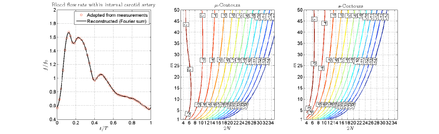
Fig. 1: Blood flow within ICA. (Left) Normalized flow rate $f/f_{0}$: data, adapted from [29], are plotted against Fourier reconstruction based on $M=15$ modes. (Middle) Contour plots for $\mu(m,N)$: e.g. it is necessary to choose $2N=34$ for the relative magnitude of discarded modes to be below $10^{-12}$, for all the considered $m$ values. (Right) Contour plots for $s(m,N)$: e.g. it is necessary to choose $2N=28$ to get a relative sensitivity to truncation below $10^{-12}$, for all the considered $m$ values.

An average radius for such a vessel is $0.25$ cm [34]. Hence, by assuming e.g. an eccentricity equal to $0.6$, we consistently introduced an elliptical cross-section with semi-axes $\alpha=0.25$ [cm] and $\beta=0.15$ [cm], being the corresponding $\eta$-range $E^{\prime}_{\eta}=[0,b]$, with $b=0.69$ (a more realistic vessel deformation, e.g. due to compression by the surrounding tissue, might imply some larger value for $\alpha$; however such a refined estimate is beyond the scope of the present simulations). Furthermore, a characteristic diameter for the considered section is $\tilde{\delta}=\alpha+\beta=0.4$ [cm], while the section-averaged speeds is $\bar{w}=f_{0}/A=34.9$ [cm/s], where $A=\pi\alpha\beta$ represents the cross-sectional area. The adopted flux was then approximated by $M=15$ modes; corresponding Fourier sum, also reported in Fig. 1, suitably replaces the data at hand (associated Pearson correlation coefficient differs from $1$ by less than $10^{-3}$). Moreover, once introduced a characteristic speed $\tilde{w}=A^{-1}\max_{t/T\in[0,1]}f(t)=58.36$ [cm/s] and by assuming $\nu=3.5\cdot 10^{-2}$ [cm²/s] [50], it is possible to label the considered blood flow with a Reynolds number $Re=\tilde{w}\tilde{\delta}/\nu\cong 670$. In addition, once defined a characteristic frequency $\widetilde{\omega}=\left(\sum_{m=0}^{M}|\widehat{f}_{m}|\,\omega_{m}\right)/\left(\sum_{m=0}^{M}|\widehat{f}_{m}|\right)$, it is possible to also introduce a characteristic Womersley number, namely $\mathrm{Wo}=(\tilde{\delta}/2)\sqrt{\widetilde{\omega}/\nu}\cong 1.5$. Despite the scarcity of results on stability for pulsatile flows (which seem to be often contradictory with one another already for the circular cross-section [54]), the above figures suggest that the flow at hand is laminar. This was derived by considering available experimental thresholds for the circular cross-section [11, 25], possibly defined through empirical fittings as in [42] (to the purpose, it may be appropriate to also define relevant Reynolds and Womersley numbers in a slightly different way [11], yet we verified that this does not affect the above statement on stability for the considered flow). That said, more detailed considerations on laminar stability cannot be drawn in the present scope: they certainly require more consolidated acquisitions, as expressly remarked e.g. in [11]. Step (S2) of the procedure proposed in Section 3.3 was then addressed, by choosing $M^{\star}=50$ for the sake of illustration. More in detail, the contours shown in Fig. 1 were firstly derived for both $\mu(m,N)$ and $s(m,N)$, respectively defined in (21) and (22), for $m=1,\ldots,M^{\star}$ and $N$ large enough. To the purpose, we coded the boundary value problem (19) within Matlab environment and we solved it by a shooting technique. As a result, by choosing e.g. $\bar{\mu}=\bar{s}=10^{-12}$, it is immediate to get $N^{\star}_{\bar{\mu}}=17$ and $N^{\star}_{\bar{s}}=14$ from the relevant plots in Fig. 1, so as to finally determine $N^{\star}=17$. Please also notice how, for any fixed $m$, $\|\widehat{v}_{m,n}\|_{\infty}\geq\|\widehat{v}_{m,n+2}\|_{\infty}$ for $n=0,...,2N-2$, thus confirming the expected relative less influence of higher $n$-modes. Relevant modes $\widehat{v}_{m,n}$ were thus obtained by solving (19) with $N=N^{\star}$; Fig 2 shows some solution components, including $\varphi_{1}$ defined in (25).

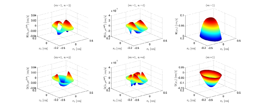
Fig. 2: Blood flow within ICA. Real part (upper row) and imaginary part (lower row) of selected solution components, computed with $2N=34$: $\widehat{v}_{1,2}(\eta)e^{i2\theta}$ (left column), $\widehat{v}_{1,4}(\eta)e^{i4\theta}$ (middle column) and $\varphi_{1}(\eta,\theta)$ (right column). Latter quantity, defined in (25), accounts in particular for all the $m=1$ modes.

We then compared our numerical results with those achieved by means of the commercial finite element (FE) solver ADINA 8.8.1 (ADINA R$\&$D Inc., MA, USA), available to the group. Such a solver uses a standard Galerkin formulation (stabilized by upwinding for higher Reynolds numbers [4]), while time-advancing is implemented by a first-order Euler backward method. As for FE simulations, a pipe with length $\ell=160\tilde{\delta}$ was defined, in order to obtain a fully-developed flow in the central portion of the domain (such a condition was a posteriori checked). Furthermore, the flow rate shown in Fig 1 was imposed (by software coding) at the inlet cross-section, the no-slip (i.e. Dirichlet) boundary condition was enforced on vessel wall, and a reference pressure value was imposed at the outlet cross-section (such value is immaterial, due to the incompressible formulation). In addition, as regards simulation set-up, both space- and time-discretization were incrementally refined, up to obtain discretization-independent results. In particular, pipe domain was discretized by nearly $8.2\cdot 10^{5}$ second-order accurate brick elements, and $7$ pulsation periods were simulated (time-periodicity was obtained after $4$ periods). Finally, all simulations were run on a single core of a PC with Intel Core i7-960 3.20 GHz CPU and 24 GB RAM. Obtained results are shown in Fig 3; as expected, a very good agreement is achieved between the considered approaches, main difference residing in computational times. Indeed, once accomplished in roughly $3$ minutes the preliminary step (S2) (see Section 3.3) so as to get truncation-independent results, the computation is finalized in a very few seconds. Conversely, runtime for the FE simulation was about $9$ days; additional days were necessary to set-up the simulation (namely to get grid-independence, periodicity and fully-developed flow conditions), so that the overall computational time for the FE run can be estimated over $20$ days. Corresponding speed-up factor is close to $10^{4}$.

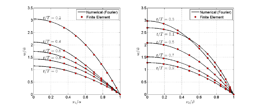
Fig. 3: Blood flow within ICA. Normalized velocity profiles $w/\bar{w}$ along the major (left) and minor (right) semi-axes of the ellipse, for selected non-dimensional times $t/T$. Results obtained by the proposed Fourier-based approach (solid curves) are compared with those achieved by a commercial FE solver (filled circles).

4.2 Cerebrospinal fluid flow in the spine

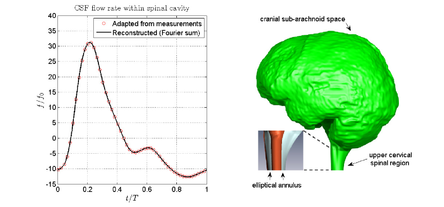
Fig. 4: CSF flow in the spine. (Left) Normalized flow rate $f/f_{0}$: data, adapted from [24], are plotted against Fourier reconstruction based on $M=15$ modes. (Right) 3D Reconstruction of the CSF domain, as obtained from patient-specific magnetic resonance imaging (MRI). Cranial sub-arachnoid space [31] and upper cervical spinal region are shown; location of the considered annulus is shown in the inset.

A flow rate waveform for cerebrospinal fluid (CSF) in the upper cervical region of the human spine [31]) was adapted from [24], see Fig 4; corresponding period-averaged flow rate is $f_{0}=-0.11$ [cm³/s] (negative sign here indicates that it is directed towards the lumbar region). Corresponding period was assumed equal to that one of the cardiac cycle, reported in Section 4.1. The considered cross-section can be approximated by the annulus between two confocal ellipses with $\alpha_{2}=1.11$ [cm], $\beta_{2}=0.93$ [cm] (from which $a=0.61$ [cm]) and $\beta_{1}=0.43$ [cm], being the corresponding $\eta$-range $E^{\prime}_{\eta}=[b_{1},b_{2}]$, with $b_{1}=0.66$ and $b_{2}=1.21$. Furthermore, a characteristic thickness for the considered section is $\tilde{\tau}=\left(\alpha_{2}-\alpha_{1}+\beta_{2}-\beta_{1}\right)/2=0.43$ [cm], while the section-averaged speeds is $\bar{w}=f_{0}/A=-0.47$ [cm/s], where $A$ represents the cross-sectional area. Such a flux was then approximated by $M=15$ modes; corresponding Fourier sum, also reported in Fig. 4, suitably replaces the data at hand (associated Pearson correlation coefficient differs from $1$ by less than $10^{-6}$). Moreover, by reasoning as in Section 4.1 with $\tilde{\tau}$ in place of $\tilde{\delta}$, and by assuming $\nu=10^{-2}$ [cm²/s] [37], it is possible to label the considered blood flow with a Reynolds number $Re=\tilde{w}\tilde{\tau}/\nu\cong 64$ and a Womersley number $\mathrm{Wo}=(\tilde{\tau}/2)\sqrt{\widetilde{\omega}/\nu}\cong 5.5$. In light of the relevant references introduced in Section 4.1, the above figures suggest that the flow at hand is laminar. However, also in this case more consolidated results are needed for a stronger statement on stability (available data for the circular cross-section [54, 11] better describe almost purely oscillating flows like the present one, yet not in an annular section); such a study is clearly beyond the present scope. By proceeding as for the ICA, we then determined $N^{\star}$ by considering $M^{\star}=50$ $m$-modes: once chosen $\bar{\mu}=\bar{s}=10^{-12}$ we got $N^{\star}=17$ (associated contours are not shown for brevity, being similar to those in Fig 1). Relevant modes $\widehat{v}_{m,n}$ were thus obtained by solving (19) with $N=N^{\star}$; Fig 5 shows some solution components, including $\varphi_{1}$ defined in (25).

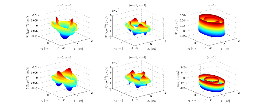
Fig. 5: CSF flow in the spine. Real part (upper row) and imaginary part (lower row) of selected solution components, computed with $2N=34$: $\widehat{v}_{1,2}(\eta)e^{i2\theta}$ (left column), $\widehat{v}_{1,4}(\eta)e^{i4\theta}$ (middle column) and $\varphi_{1}(\eta,\theta)$ (right column). Latter quantity, defined in (25), accounts in particular for all the $m=1$ modes.

As for the ICA test-case, we compared our numerical results with those achieved by the commercial solver ADINA (relevant details can be recalled from Section 4.1). For such FE simulations, a pipe with length $\ell\cong 100\bar{\tau}$ was defined, in order to obtain a fully-developed flow in the central portion of the domain (such a condition was a posteriori checked). Furthermore, the flow rate shown in Fig 4 was imposed (by software coding) at the inlet cross-section, the no-slip (i.e. Dirichlet) boundary condition was enforced on vessel walls, and a reference pressure value was imposed at the outlet cross-section (such value is immaterial, due to the incompressible formulation). In addition, as regards simulation set-up, both space- and time-discretization were incrementally refined, up to obtain discretization-independent results. In particular, pipe domain was discretized by nearly $3.8\cdot 10^{5}$ second-order accurate brick elements, and $7$ pulsation periods were simulated (time-periodicity was obtained after $2$ periods). Obtained results are shown in Fig 6 (they are obviously identical to those reported in [24]). As expected, a very good agreement is achieved between the proposed Fourier-based solution and that provided by the finite element solver, main difference residing in computational times for the present case as well. Indeed, once accomplished in roughly $3$ minutes the preliminary step (S2) (see Section 3.3) so as to get truncation-independent results, the computation is finalized in a very few seconds. Conversely, runtime for the FE simulation was about $4$ days (less than for ICA thanks to the lower average speeds); additional days were necessary to set-up the simulation (namely to get grid-independence, periodicity and fully-developed flow conditions), so that the overall computational time for the FE run can be estimated over $10$ days. Corresponding speed-up factor is well over $10^{3}$ also in the present case.

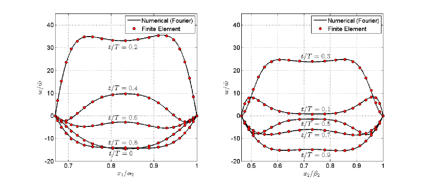
Fig. 6: CSF flow in the spine. Normalized velocity profiles $w/\bar{w}$ along the major (left) and minor (right) semi-axes of the annulus, for selected non-dimensional times $t/T$. Results obtained by the proposed Fourier-based approach (solid curves) are compared with those achieved by a commercial FE solver (filled circles).

5 Concluding remarks

We proposed a novel numerical method for solving the inverse problem of pulsatile viscous flows in elliptical vessels and annuli. In particular, we addressed a fully-developed flow of an incompressible Newtonian fluid, so as preliminarily derive some analytical relations (otherwise hardly achievable) upon which to build our numerical solution. We are therefore aware of the fact that the solution we propose is hardly applicable to 3D finite-length complex domains (such a limitation, despite being obvious, is often understated by the many authors who also assumed a fully-developed flow). On regard, under quite general assumptions (yet still adopting an incompressible Newtonian fluid), many valuable approaches for problems with flow rate conditions have been proposed in the literature (see e.g. [18]), and they are the subject of ongoing research. Moreover, a fully numerical approach is the only viable when also considering non-Newtonian fluids, already when tackling stationary problems (possibly within curved or non-straight vessels as in [2]). Nevertheless, and in spite of the linear context within which it was derived, our solution to the considered inverse problem is original and non-trivial. Indeed, it provides an easily computable benchmark (as well as an approximation) for such a problem. In particular, by invoking separation of variables (in elliptical coordinates) we obtained a tridiagonal system of linear, ordinary differential equations and we obtained the sought solution by means of a Galerkin-type truncation. This method seem to theoretically corroborate the early attempts in [49] (in which proper references to the inverse problem are missing). Moreover, it represents an alternative to the numerical approach in [24], heavily based on a wise computation strategy of the Mathieu functions. Indeed, truncation of the aforementioned system represents the differential counterpart of the truncation of the infinite dimensional algebraic linear system in [24], which is performed in order to evaluate corresponding eigenvalues. In this sense, we only indirectly referred to Mathieu functions, thus circumventing the numerical challenges associated therewith (see [24, 26, 53]). As a consequence, even if the considered differential system is not completely integrable (due to the coupling between Fourier modes which is implied by the elliptical cross-section already when addressing the stationary problem), our solution can be easily computed, even for small ellipticity values. Such an asset was shown through the numerical simulations reported in Section 4, based on measured flow rates for blood in the internal carotid artery (ICA), and cerebrospinal fluid (CSF) flow in the upper cervical region of the human spine. Indeed, despite being expected, the main advantage of the proposed method, as compared to fully numerical approaches, resides in computational efficiency: a speed-up over $10^{3}$ was obtained for both the aforementioned test-cases. Such a gain is comparable with the one reported in [24], even if simulation set-up times seem to be slightly understated therein (in particular, computation of the Mathieu functions was recognized as the most critical part, and several related convergence results are reported in such a valuable paper, yet at the same time corresponding computational burden was judged as inexpensive [24]). An additional, potential advantage of the proposed Fourier-based approach resides in the possibility of an extensive and detailed control over numerical implementation (as opposite to black-box libraries usually exploited for computing special functions), which could be further optimized e.g. by using consolidated techniques for Fast Fourier solvers [23].

These results effectively support the exploitation of the proposed method in a wider research scope, e.g. as a debugging tool and/or an improved source of boundary data for more ambitious numerical approaches, possibly based on more realistic data. On regard and with reference to the study of blood flow, the proposed solution could provide an enhanced inflow condition for those approaches which merely scale a (steady) parabolic solution by a factor accounting for flow rate variability (see e.g. [22]). Moreover, the proposed solution can be directly used for computing wall shear stress distribution along the adopted cross-section boundary. Indeed, vessel ellipticity affects such a stress [26], which in turn has been identified as a key player in the onset and development of relevant pathologies likes atherosclerosis, even if several acquisitions needs to be consolidated (see e.g. [49, 10]). Furthermore, still within the context of bio-fluid dynamics, many investigations are being carried out for elucidating the role of CSF dynamics within human spine, in relation to the onset and progression of relevant diseases like syringomyelia. The proposed benchmark flow holds potential for application to such studies as well, in particular for assigning more accurate inflow/initial conditions in the cervical portion of the spinal fluid domain (which is usually described as a circular annulus between two finite-length, compliant cylinders [8, 14, 16]; wave propagation is usually studied therein). It is worth mentioning that relevant investigations for such fluid-structure interaction problems are being performed in the context of hemodynamics as well (see e.g. [9]). Furthermore, besides studies purely focusing on fluid dynamics, the proposed solution can be effectively applied to additional biomedical applications (as anticipated, the biomedical field is an elective application domain, since flow rate is a main available physical datum), e.g. to targeted delivery problems. For instance, the effect of flow pulsatility on magnetic particle targeting was originally exemplified in [6], in order to highlight peculiar effects with respect to the stationary case [27] widely adopted when addressing particle targeting in blood capillaries. Such an enhancement straightforwardly applies to magnetoresponsive carriers at large, e.g. to the controlled navigation of MRI-guided microrobots in the vasculature [3]. Indeed, there is a growing interest in the robotic field for the development of micro/miniaturized interventional tools to be navigated (e.g. through magnetic fields) within bodily fluids. These systems, currently defined as microrobots  [41] despite their intrinsic simplicity (system compartmentalization is indeed almost inapplicable at the micro scale), hold potential for effective application to medical fields, and both blood flow and CSF flow were identified as elective carrying fluids. To further support this point, it is worth mentioning that, besides carrier transport along the mainstream, active microrobot navigation was also proposed, e.g. in the CSF flow. More precisely, magnetic navigation of helical microrobots was proposed for application in the spinal CSF [19] (being the helical shape inspired by the propulsion strategy of bacterial flagella, well suited for low-Reynolds-number regimes). Interestingly, relevant CSF velocity profile, together with corresponding fluidic actions on the microrobot, seem to be slightly overlooked in these studies (while attention is payed to other physical aspects, up to gravity, in spite of its minor effects at the micro scale [39]). This seems to be partly due to the lack of easily computable - yet physically derived - flow conditions; such an issue might be mitigated by our benchmark flow solution, thus contributing to better assess the feasibility of such long-term approaches in bodily fluids, even if still in a simplified context. Finally, an additional, remarkable application field has been recently identified, namely the one of energy harvesting from bodily fluids. Indeed, use of magnetic fields was proposed as a key powering strategy for most of the aforementioned microrobots, mainly in response to the impossibility of using on-board batteries at the micro scale (alternative approaches based on harnessing the power of biological entities like bacteria were also proposed, yet their discussion is out of the present scope). In fact, powering (closely linked to actuation) appears as the real bottleneck currently hampering microrobotic applications, and energy harvesting holds promise to solve such a major issue. In this spirit yet in the wider context of implantable miniaturized electronic devices for biomedical applications, an implantable fuel cell has been recently proposed [45], powered through energy scavenging from the CSF. Relevant estimates are reported in the cited reference in order to assess powering effective sustainability (they address oxygen and glucose transport within the CSF domain, mainly in the brain region but also encompassing the spinal one). However, it is expressly recognized in [45] that a deeper insight into the actual CSF dynamics is required to accurately assess the performance of the proposed system. Such a quest further supports the development of modeling strategies for the CSF flow (yet such a point can be immediately extended to other fluid conditions), and the benchmark flow solution we propose, despite the inherent simplifications we repeatedly pointed out above, could contribute to take a leap ahead in many of the aforementioned applications areas.

To conclude, while developing the proposed numerical method we deliberately sacrificed some degree of physiological representativeness, yet in the name of direct and efficient computability, and thus wider usability of the obtained benchmark flow solution. The many applications discussed above encourage to exploit our solution in an wide interdisciplinary context, so as to further push the corresponding scientific and technological frontiers.

References

- [1] F. A. Alhargan, A complete method for the computations of Mathieu characteristic numbers of integer orders, SIAM Rev., 38 (1996), pp. 239–255.
- [2] N. Arada, M. Pires, and A. Sequeira, Viscosity effects on flows of generalized Newtonian fluids through curved pipes, Comput. Math. Appl., 53 (2007), pp. 625–646.
- [3] L. Arcese, M. Fruchard, F. Beyeler, A. Ferreira, and B. J. Nelson, Adaptive backstepping and MEMs force sensor for an MRI-guided microrobot in the vasculature, in Proceedings of 2011 IEEE International Conference on Robotics and Automation, Shanghai, China, May 2011, pp. 4121–4126.
- [4] K. J. Bathe, H. Zhang, and M. H. Wang, Finite element analysis of incompressible and compressible fluid flows with free surfaces and structural interactions, Comput. Struct., 56 (1995), pp. 193–213.
- [5] H. Beirão da Veiga, Time periodic solutions of the Navier-Stokes equations in unbounded cylindrical domains—Leray’s problem for periodic flows, Arch. Ration. Mech. Anal., 178 (2005), pp. 301–325.
- [6] L. C. Berselli, P. Miloro, A. Menciassi, and E. Sinibaldi, Exact solution to the inverse Womersley problem for pulsatile flows in cylindrical vessels, with application to magnetic particle targeting, Appl. Math. Comput. (doi: 10.1016/j.amc.2012.11.071), (2012, in press).
- [7] L. C. Berselli and M. Romito, On Leray’s problem for almost periodic flows, J. Math. Sci. Univ. Tokyo, 19 (2012), pp. 69–130.
- [8] C. D. Bertram, A numerical investigation of waves propagating in the spinal cord and subarachnoid space in the presence of a syrinx, J. Fluids Struct., 25 (2009), pp. 1189–1205.
- [9] S. Čanić, J. Tambaca, G. Guidoboni, A. Mikelic, C. Hartley, and D. Rosenstrauch, Modeling viscoelastic behavior of arterial walls and their interaction with pulsatile blood flow, SIAM J. Appl. Math., 67 (2006), pp. 164–193.
- [10] C. G. Caro, Discovery of the role of wall shear in atherosclerosis, Arterioscler Thromb Vasc Biol., 29 (2009), pp. 158–161.
- [11] M. Ö. Çarpinlioglu and M. Y. Gündogdu, A critical review on pulsatile pipe flow studies directing towards future research topics, Flow Meas. Instrum., 12 (2001), pp. 163–174.
- [12] G. Chen, P. J. Morris, and J. Zhou, Visualization of special eigenmode shapes of a vibrating elliptical membrane, SIAM Rev., 36 (1994), pp. 453–469.
- [13] S. Cheng, M. A. Stoodley, J. Wong, S. Hemley, D. F. Fletcher, and L. E. Bilston, The presence of arachnoiditis affects the characteristics of CSF flow in the spinal subarachnoid space: a modelling study, J. Biomech., 45 (2012), pp. 1186–91.
- [14] S. Cirovic and M. Kim, A one-dimensional model of the spinal cerebrospinal-fluid compartment, J. Biomech. Eng., 134 (2012), p. 021005.
- [15] C. Di Rocco, P. Frassanito, L. Massimi, and S. Peraio, Hydrocephalus and Chiari type I malformation, Childs Nerv. Syst., 27 (2011), pp. 1653–64.
- [16] N. S. J. Elliott, Syrinx fluid transport: Modeling pressure-wave-induced flux across the spinal pial membrane, J. Biomech. Eng., 134 (2012), p. 31006.
- [17] L. Formaggia, A. Quarteroni, and A. Veneziani, The circulatory system: from case studies to mathematical modeling, in Complex systems in biomedicine, Springer Italia, Milan, 2006, pp. 243–287.
- [18] L. Formaggia, A. Veneziani, and C. Vergara, Flow rate boundary problems for an incompressible fluid in deformable domains: formulations and solution methods, Comput. Methods Appl. Mech. Engrg., 199 (2010), pp. 677–688.
- [19] T. W. R. Fountain, P. V. Kailat, and J. J. Abbott, Wireless control of magnetic helical microrobots using a rotating-permanent-magnet manipulator, in Proceedings of 2010 IEEE International Conference on Robotics and Automation, Anchorage, AK, USA, May 2010, pp. 576–581.
- [20] G. P. Galdi, An introduction to the mathematical theory of the Navier-Stokes equations. Vol. I, vol. 38 of Springer Tracts in Natural Philosophy, Springer-Verlag, New York, 1994. Linearized steady problems.
- [21] G. P. Galdi and A. M. Robertson, The relation between flow rate and axial pressure gradient for time-periodic Poiseuille flow in a pipe, J. Math. Fluid Mech., 7 (2005), pp. S215–S223.
- [22] A. Gizzi, M. Bernaschi, D. Bini, C. Cherubini, S. Filippi, S. Melchionna, and S. Succi, Three-band decomposition analysis of wall shear stress in pulsatile flows, Phys. Rev. E, 83 (2011), p. 031902.
- [23] L. Greengard and J.-Y. Lee, Accelerating the nonuniform fast Fourier transform, SIAM Rev., 46 (2004), pp. 443–454.
- [24] S. Gupta, D. Poulikakos, and V. Kurtcuoglu, Analytical solution for pulsatile viscous flow in a straight elliptic annulus and application to the motion of the cerebrospinal fluid, Phys. Fluids, 20 (2008), p. 093607.
- [25] K. Haddad, O. Ertunç, M. Mishra, and A. Delgado, Pulsating laminar fully developed channel and pipe flows, Phys. Rev. E, 81 (2010), p. 016303.
- [26] M. Haslam and M. Zamir, Pulsatile flow in tubes of elliptic cross sections, Ann. Biomed. Eng., 26 (1998), p. 780.
- [27] J. W. Haverkort, S. Kenjere, and C. R. Kleijn, Magnetic particle motion in a Poiseuille flow, Phys. Rev. E, 80 (2009), p. 016302.
- [28] S. Hentschel, K.-A. Mardal, A. E. Lovgren, S. Linge, and V. Haughton, Characterization of Cyclic CSF Flow in the Foramen Magnum and Upper Cervical Spinal Canal with MR Flow Imaging and Computational Fluid Dynamics, Am. J. Neuroradiol., 31 (2010), pp. 997–1002.
- [29] Y. Hoi, B. A. Wasserman, Y. Y. J. Xie, S. S. Najjar, L. Ferruci, E. G. Lakatta, G. Gerstenblith, and D. A. Steinman, Characterization of volumetric flow rate waveforms at the carotid bifurcations of older adults, Physiol. Meas., 31 (2010), pp. 291–302.
- [30] H.-F. Huang and C.-L. Lai, Enhancement of mass transport and separation of species by oscillatory electroosmotic flows, Proc. R. Soc. Lond. Ser. A Math. Phys. Eng. Sci., 462 (2006), pp. 2017–2038.
- [31] D. N. Irani, Cerebrospinal Fluid in Clinical Practice, Saunders, 2008.
- [32] S. R. Khamrui, On the flow of a viscous liquid through a tube of elliptic section under the influence of a periodic pressure gradient, Bull. Calcutta Math. Soc., 49 (1957), pp. 57–60.
- [33] A. Korichi, L. Oufer, and G. Polidori, Heat transfer enhancement in self-sustained oscillatory flow in a grooved channel with oblique plates, Int. J. Heat Mass Transfer, 52 (2009), pp. 1138–1148.
- [34] J. Krejza, M. Arkuszewski, S. E. Kasner, J. Weigele, A. Ustymowicz, R. W. Hurst, B. L. Cucchiara, and S. R. Messe, Carotid Artery Diameter in Men and Women and the Relation to Body and Neck Size, Stroke, 37 (2006), pp. 1103–5.
- [35] M.-C. Lai, Fast direct solver for Poisson equation in a 2D elliptical domain, Numer. Methods Partial Differential Equations, 20 (2004), pp. 72–81.
- [36] A. A. Linninger, M. Xenos, B. Sweetman, S. Ponkshe, X. Guo, and R. Penn, A mathematical model of blood, cerebrospinal fluid and brain dynamics, J. Math. Biol., 59 (2009), pp. 729–759.
- [37] F. Loth, M. A. Yardimci, and N. Alperin, Hydrodynamic modeling of cerebrospinal fluid motion within the spinal cavity, J. Biomech. Eng., 123 (2001), pp. 71–79.
- [38] M. Loukas, B. J. Shayota, K. Oelhafen, J. H. Miller, J. J. Chern, R. S. Tubbs, and W. J. Oakes, Associated disorders of Chiari Type I malformations: a review, Neurosurg Focus, 31 (2011), p. E3.
- [39] A. W. Mahoney, J. C. Sarrazin, E. Bamberg, and J. J. Abbott, Velocity control with gravity compensation for magnetic helical microswimmers, Advanced Robotics, 25 (2011), pp. 1007–1028.
- [40] N. W. McLachlan, Theory and application of Mathieu functions, Clarendon Press, 1947.
- [41] B. J. Nelson, I. K. Kaliakatsos, and J. J. Abbott, Microrobots for minimally invasive medicine, Annu. Rev. Biomed. Eng., 12 (2010), pp. 55–85.
- [42] J. Peacock, T. Jones, C. Tock, and R. Lutz, The onset of turbulence in physiological pulsatile flow in a straight tube, Exp. Fluids, 24 (1998), pp. 1–9.
- [43] K. Pileckas, The Navier-Stokes system in domains with cylindrical outlets to infinity. Leray’s problem, in Handbook of mathematical fluid dynamics, Vol. IV, North-Holland, Amsterdam, 2007, pp. 445–647.
- [44] S. B. Pope, Turbulent flows, Cambridge University Press, Cambridge, 2000.
- [45] B. I. Rapoport, J. T. Kedzierski, and R. Sarpeshkar, A glucose fuel cell for implantable brainmachine interfaces, PLoS ONE, 7 (2012), p. e38436.
- [46] Y. V. K. Ravi Kumar, P. S. V. H. N. Krishna Kumari, M. V. Ramana Murthy, and S. Sreenadh, Unsteady peristaltic pumping in a finite length tube with permeable wall, J. Fluids Eng., 132 (2010), p. 101201.
- [47] S. Ray and F. Durst, Semianalytical solutions of laminar fully developed pulsating flows through ducts of arbitrary cross sections, Phys. Fluids, 16 (2004), p. 4371.
- [48] A. M. Robertson, A. Sequeira, and R. G. Owens, Rheological models for blood, in Cardiovascular mathematics, vol. 1 of MS&A. Model. Simul. Appl., Springer Italia, Milan, 2009, pp. 211–241.
- [49] M. B. Robertson, U. Köhler, P. R. Hoskins, and I. Marshall, Flow in elliptical vessels calculated for a physiological waveform, J. Vasc. Res., 38 (2001), pp. 73–82.
- [50] K. Rogers, Blood: Physiology and Circulation, Human Body, Rosen Publishing Group, 2010.
- [51] T. Sexl, Uber den von E. G. Richardson entdeckten “Annulareffekt”, Z. Phys, 61 (1930), pp. 179–221.
- [52] N. Shaffer, B. Martin, and F. Loth, Cerebrospinal fluid hydrodynamics in type I Chiari malformation, Neurol. Res., 33 (2011), pp. 247–260.
- [53] J. Shen and L.-L. Wang, On spectral approximations in elliptical geometries using Mathieu functions, Math. Comp., 78 (2009), pp. 815–844.
- [54] R. Trip, D. J. Kuik, J. Westerweel, and C. Poelma, An experimental study of transitional pulsatile pipe flow, Phys. Fluids, 24 (2012), p. 014103.
- [55] P. D. Verma, The pulsating viscous flow superposed on the steady laminar motion of incompressible fluid between two co-axial cylinders, Proc. Indian Acad. Sci. Math. Sci., 26 (1960), pp. 447–458.
- [56] , The pulsating viscous flow superposed on the steady laminar motion of incompressible fluid in a tube of elliptic section, Proc. Indian Acad. Sci. Math. Sci., 26 (1960), pp. 282–297.
- [57] M. E. Wagshul, P. K. Eide, and J. R. Madsen, The pulsating brain: A review of experimental and clinical studies of intracranial pulsatility, Fluids Barriers CNS, 8 (2011), p. 5.
- [58] X. Wang and N. Zhang, Numerical analysis of heat transfer in pulsating turbulent flow in a pipe, Int. J. Heat Mass Transfer, 48 (2005), pp. 3957–3970.
- [59] J. R. Womersley, Method for the calculation of velocity, rate of flow and viscous drag in arteries when the pressure gradient is known, J. Physiol., 127 (1955), pp. 553–563.