Dynamics of the Bianchi I model with non-minimally coupled scalar field near the singularity

Abstract

Dynamical systems methods are used to study the evolution of the Bianchi I model with a scalar field. We show that inclusion of the non-minimal coupling term between the scalar field and the curvature changes evolution of the model compared with the minimally coupled case. In the model with the non-minimally coupled scalar field there is a new type of singularity dominated by the non-minimal coupling term. We examine the impact of the non-minimal coupling on the anisotropy evolution and demonstrate the existence of its minimal value in the generic case.

1 Introduction

In the simplest cosmological model with a scalar field one can introduce a term modelling its coupling with the curvature. Such a term appears naturally if we understand the General Relativity as an effective field theory of gravity Donoghue (1994). To answer the question how stable effects of the non-minimal coupling are, we consider the simplest anisotropic space of Bianchi I type which represents the simplest flat model with anisotropy.

In the model under consideration we assume a universe filled with a non-minimally coupled scalar field with the curvature and an unknown coupling constant $\xi$. The action assumes the following form

$$\begin{split}S=&\frac{1}{2\kappa^{2}}\int\mathrm{d}^{4}x\sqrt{-g}R\\ &-\frac{1}{2}\int\mathrm{d}^{4}x\sqrt{-g}\left\{\varepsilon\nabla^{\alpha}\phi\,\nabla_{\alpha}\phi+\varepsilon\xi R\phi^{2}+2U(\phi)\right\}\end{split}$$ (1)

where $\kappa^{2}=8\pi G$, $\varepsilon=\pm 1$ corresponds to a canonical and phantom scalar field, respectively, the metric signature is $(-,+,+,+)$ and $U(\phi)$ is the scalar field potential function assumed in a polynomial form.

2 Bianchi I metric

We assume the following form of the metric

$$\mathrm{d}s^{2}=-\mathrm{d}t^{2}+a^{2}(t)\Big{(}g_{1}^{2}(t)\mathrm{d}x^{2}+g_{2}^{2}(t)\mathrm{d}y^{2}+g_{3}^{2}(t)\mathrm{d}z^{2}\Big{)}\,,$$ (2)

together with the condition

$$g_{1}g_{2}g_{3}=1\,.$$ (3)

The energy conservation condition we obtain from variation of the action (1) with respect to the metric components

$$\begin{split}3H^{2}-\Sigma=\kappa^{2}\Big{(}&\varepsilon\frac{1}{2}\dot{\phi}^{2}+U(\phi)\\ &+\varepsilon\xi(3H^{2}-\Sigma)\phi^{2}+\varepsilon 3\xi H(\phi^{2})\dot{}\Big{)}\end{split}$$ (4)

where the anisotropy is measured by

$$\begin{split}\Sigma&=\frac{1}{2}\left(\left(\frac{\dot{g_{1}}}{g_{1}}\right)^{2}+\left(\frac{\dot{g_{2}}}{g_{2}}\right)^{2}+\left(\frac{\dot{g_{3}}}{g_{3}}\right)^{2}\right)\\ &=\frac{1}{2}\left(q_{1}^{2}+q_{2}^{2}+q_{3}^{2}\right)\,,\end{split}$$ (5)

the Hubble function is given by $H=\frac{\dot{a}}{a}$ and the space volume is $V=a^{3}$.

The acceleration equation is

$$\begin{split}\dot{H}=&-2H^{2}-\frac{1}{3}\Sigma+\\ &+\frac{\kappa^{2}}{6}\frac{-\varepsilon(1-6\xi)\dot{\phi}^{2}+4U(\phi)-6\xi\phi U^{\prime}(\phi)}{1-\varepsilon\xi(1-6\xi)\kappa^{2}\phi^{2}}\,.\end{split}$$ (6)

From space-space Einstein’s equations we have additional equations of motion for anisotropy

$$(1-\varepsilon\xi\kappa^{2}\phi)\dot{q_{i}}=\varepsilon\xi\kappa^{2}q_{i}(\phi^{2})\dot{}-3Hq_{i}(1-\varepsilon\xi\kappa^{2}\phi^{2})\,.$$ (7)

When the non-minimal coupling is present one can write the right hand sides of Einstein field equations in several possible inequivalent ways Faraoni (2004). In the case adopted here the energy momentum tensor of the scalar field is covariantly conserved, which may not be true for different approaches. For example, one can redefine the gravitational constant $\kappa_{\text{eff}}^{-2}=\kappa^{-2}-\varepsilon\xi\phi^{2}$ making it time dependent, then the effective gravitational constant can diverge for a critical value of the scalar field $\phi_{c}=\pm 1/\sqrt{\varepsilon\kappa^{2}\xi}$ and the model is unstable there with respect to arbitrary small anisotropy perturbations which become infinite there Starobinsky (1981).

In what follows we introduce the energetic (expansion normalised) variables

$$x\equiv\frac{\kappa}{\sqrt{6}}\frac{\dot{\phi}}{H}\,,\quad y\equiv\frac{\kappa}{\sqrt{3}}\frac{\sqrt{U_{0}}}{H}\,,\quad z\equiv\frac{\kappa}{\sqrt{6}}\phi\,,\quad\Omega_{\Sigma}=\frac{\Sigma}{3H^{2}}\,,$$

and $U(\phi)\to f(z)$, then the energy conservation condition can be expressed as

$$\begin{split}1=&\hskip 2.84526pty^{2}f(z)+\varepsilon(1-6\xi)x^{2}+\varepsilon 6\xi(x+z)^{2}+\\ &+(1-\varepsilon 6\xi z^{2})\Omega_{\Sigma}\,,\end{split}$$ (8)

and the acceleration equation

$$\begin{split}\frac{\dot{H}}{H^{2}}=&-2-\Omega_{\Sigma}-\\ &-\frac{\varepsilon(1-6\xi)x^{2}-y^{2}\big{(}2f(z)-3\xi zf^{\prime}(z)\big{)}}{1-\varepsilon 6\xi(1-6\xi)z^{2}}\,.\end{split}$$ (9)

The equations of motion for the anisotropy are

$$(1-\varepsilon 6\xi z^{2})\frac{1}{H}\frac{\dot{q_{i}}}{q_{i}}=\varepsilon 12\xi xz-3(1-\varepsilon 6\xi z^{2})$$ (10)

Note that for the minimally coupled scalar field $\xi=0$ equations (7) and (10) can be directly integrated and the evolution of the anisotropy does not depend whether the universe is filled with a canonical or phantom scalar field. In general case of the non-minimal coupling this is not possible because these equations depend on the phase space variables.

The dynamical system is in the following form

$$\begin{split}\frac{\mathrm{d}x}{\mathrm{d}\ln{a}}&=-x(1-\Omega_{\Sigma})-\varepsilon\frac{1}{2}y^{2}f^{\prime}(z)-\\ &\quad-(x+6\xi z)\Big{(}\frac{\dot{H}}{H^{2}}+2+\Omega_{\Sigma}\Big{)}\,,\\ \frac{\mathrm{d}y}{\mathrm{d}\ln{a}}&=-y\frac{\dot{H}}{H^{2}}\,,\\ \frac{\mathrm{d}z}{\mathrm{d}\ln{a}}&=x\,.\end{split}$$ (11)

where using equations (8) and (9) we eliminate $\Omega_{\Sigma}$ and $\dot{H}/H^{2}$. One can see that right hand sides of the dynamical system (11) are rational functions of their arguments. In order to use standard dynamical systems methods we need to make the following time transformation

$$(1-\varepsilon 6\xi z^{2})(1-\varepsilon 6\xi(1-6\xi)z^{2})\frac{\mathrm{d}}{\mathrm{d}\ln{a}}=\frac{\mathrm{d}}{\mathrm{d}\tau}\,$$ (12)

which removes singularities of the system at $z^{2}=\frac{1}{\varepsilon 6\xi}$ and $z^{2}=\frac{1}{\varepsilon 6\xi(1-6\xi)}$.

In this work we concentrate our attention at the following critical point

$$(x^{*}=-6\xi z^{*},\quad y^{*}=0,\quad(z^{*})^{2}=\frac{1}{\varepsilon 6\xi(1-6\xi)})$$

which for the isotropic case corresponds to the finite scale factor singularity Hrycyna and Szydlowski (2010). The existence of this critical point depends on the value of the coupling constant $\xi$ only. For the canonical scalar field $\varepsilon=+1$ it exists for $0<\xi<\frac{1}{6}$ while for the phantom scalar field $\varepsilon=-1$ for $\xi<0$ or $\xi<\frac{1}{6}$.

Eigenvalues of the linearization matrix at this critical point are

$$\lambda_{1,2}=-\frac{36\xi^{2}}{1-6\xi}\,,\quad\lambda_{3}=-\frac{72\xi^{2}}{1-6\xi}\,.$$

Stability, in time $\tau$, of this critical point depends on the value of the coupling constant $\xi$. For $\xi<\frac{1}{6}$ the eigenvalues are negative indicating a stable critical point, while for $\xi>\frac{1}{6}$ the eigenvalues are positive which indicates an unstable critical point.

The solutions of the linearised system in the vicinity of the critical point under investigation are

$$\begin{split}x(\tau)&=x^{*}+\big{(}\Delta x+2(1-3\xi)\Delta z\big{)}\exp{(\lambda_{1}\tau)}-\\ &\quad-2(1-3\xi)\Delta z\exp{(\lambda_{3}\tau)}\,\\ y(\tau)&=y^{*}+\Delta y\exp{(\lambda_{2}\tau)}\,,\\ z(\tau)&=z^{*}+\Delta z\exp{(\lambda_{3}\tau)}\,.\end{split}$$ (13)

where $\Delta x=x^{(i)}-x^{*}$, $\Delta y=y^{(i)}-y^{*}$ and $\Delta z=z^{(i)}-z^{*}$ are displacements of the initial conditions with respect to coordinates of the critical point.

From (8) we see that at this critical point $\Omega_{\Sigma}^{*}=0$, and using the linearised solutions we have

$$\Omega_{\Sigma}(\tau)=\varepsilon 2(1-6\xi)^{2}z^{*}\Delta z\exp{(\lambda_{3}\tau)}\,.$$ (14)

On the other hand the anisotropy parameter $\Sigma=3H^{2}\Omega_{\Sigma}$ and in the energy phase space variables $\frac{1}{\kappa^{2}U_{0}}\Sigma=\frac{\Omega_{\Sigma}}{y^{2}}$. Using linearised solutions in the vicinity of this critical point we have

$$\frac{1}{\kappa^{2}U_{0}}\Sigma(\tau)=\frac{\Omega_{\Sigma}(\tau)}{(y(\tau))^{2}}=\varepsilon 2(1-6\xi)^{2}z^{*}\frac{\Delta z}{(\Delta y)^{2}}=\text{const.}$$ (15)

As long as the linear solutions are considered, one can see, that the anisotropy function is strictly constant and the value of anisotropy in the vicinity of the critical point representing the finite scale factor singularity depends on the value of the non-minimal coupling constant $\xi$ and initial conditions in the linear approximation. Of course one can feel bad about the square value of $\Delta y$ in the denominator which should vanish in the linear approximation, but in the dynamical system (11) the phase space variable $y$ appears only in a polynomial form of the second degree and one can make the following change of variables $\widetilde{y}=y^{2}$ and then the same results hold.

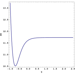
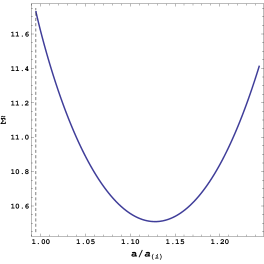
Figure 1: Evolution of the anisotropy function $\tilde{\Sigma}=\frac{\Sigma}{\kappa^{2}U_{0}}$ calculated from (8) and using $3H^{2}=\frac{\kappa^{2}U_{0}}{y^{2}}$. The initial conditions taken in the vicinity of the critical point under investigations, and $U(\phi)\propto\phi^{2}$, $\varepsilon=+1$, $\xi=\frac{1}{8}$. We observe that the anisotropy is constant at the critical point then approaches a minimal value and next grows as the universe expands. A dashed vertical line denotes value of the scale factor of the singularity.

In Figure 1 we plotted evolution of the anisotropy. At the first plot we present evolution of $\tilde{\Sigma}$ with respect to time $\tau$ and the critical point representing a finite scale factor singularity is approached at $\tau\to\infty$. At the second plot we present evolution of the anisotropy with respect to the scale factor $a/a_{(i)}$ rescaled to the value of the scale factor taken at the initial conditions.

3 Kasner metric

In this section in (2) we assume

$$g_{1}=t^{p_{1}}\,,\quad g_{2}=t^{p_{2}}\,,\quad g_{3}=t^{p_{3}}\,,$$

and the metric is

$$\mathrm{d}s^{2}=-\mathrm{d}t^{2}+a^{2}(t)\Big{(}t^{2p_{1}}\mathrm{d}x^{2}+t^{2p_{2}}\mathrm{d}y^{2}+t^{2p_{3}}\mathrm{d}z^{2}\Big{)}\,,$$ (16)

where from (3) we have constraint equation

$$p_{1}+p_{2}+p_{3}=0\,.$$

The assumed form of the metric represents a special case of the general Bianchi I metric which can be recast into the standard Kasner solution for an empty space.

Now the anisotropy function is

$$\Sigma=\frac{1}{2}(p_{1}^{2}+p_{2}^{2}+p_{3}^{2})\frac{1}{t^{2}}=3\frac{\sigma^{2}}{t^{2}}$$ (17)

and the energy conservation condition expressed in the energetic variables is

$$\begin{split}1=&\hskip 2.84526pty^{2}f(z)+\varepsilon(1-6\xi)x^{2}+\varepsilon 6\xi(x+z)^{2}+\\ &+(1-\varepsilon 6\xi z^{2})\sigma^{2}h^{2}\,,\end{split}$$ (18)

where we defined

$$h=\frac{1}{Ht}\,.$$

From (10) we obtain

$$(1-\varepsilon 6\xi z^{2})h=3(1-\varepsilon 6\xi z^{2})-\varepsilon 12\xi xz\,.$$ (19)

The dynamical system is in the following form

$$\begin{split}\frac{\mathrm{d}x}{\mathrm{d}\ln{a}}&=-x(1-\sigma^{2}h^{2})-\varepsilon\frac{1}{2}y^{2}f^{\prime}(z)-\\ &\quad-(x+6\xi z)\Big{(}\frac{\dot{H}}{H^{2}}+2+\sigma^{2}h^{2}\Big{)}\,,\\ \frac{\mathrm{d}y}{\mathrm{d}\ln{a}}&=-y\frac{\dot{H}}{H^{2}}\,,\\ \frac{\mathrm{d}z}{\mathrm{d}\ln{a}}&=x\,.\end{split}$$ (20)

where using equations (18) and (9) (after substitution $\Omega_{\Sigma}=\sigma^{2}h^{2}$) we eliminate terms containing $\sigma^{2}h^{2}$ and $\dot{H}/H^{2}$. The dynamical system describing evolution in the Kasner metric is exactly in the same form as in the case of the general Bianchi I model. One exception is the existence of the additional constraint equation (19). Using this equation we find that at the critical point under investigations $h^{*}=1$ this indicates that while a sample trajectory approaches a critical point and $H\to\infty$ then $t\to 0$.

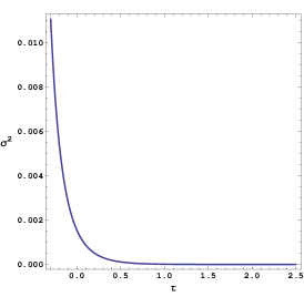
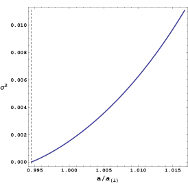
Figure 2: Evolution of the anisotropy parameter $\sigma^{2}$ calculated from (21), and $U(\phi)\propto\phi^{2}$, $\varepsilon=+1$, $\xi=\frac{1}{8}$. In the Kasner metric anisotropy vanishes at the critical point representing the finite scale factor singularity. As the universe expands anisotropy grows indicating that this critical point is unstable with respect to anisotropy perturbations. A dashed vertical line denotes value of the scale factor of the singularity.

The energy conservation condition (18) can be rewritten into the following form

$$\sigma^{2}=\frac{1-y^{2}f(z)-\varepsilon(1-6\xi)x^{2}-\varepsilon 6\xi(x+z)^{2}}{(1-\varepsilon 6\xi z^{2})h^{2}}$$ (21)

where $h$ is given by (19) and using the linearised solutions obtained in the previous section we find

$$\sigma^{2}=\varepsilon 2(1-6\xi)^{2}z^{*}\Delta z\exp{(\lambda_{3}\tau)}\,.$$ (22)

In Figure 2 we plotted evolution of the anisotropy parameter $\sigma^{2}$ for the Kasner metric. In evolution in time $\tau$ (first plot) critical point under investigations is approached as $\tau\to\infty$. At the second plot we presented evolution of $\sigma^{2}$ with respect to the scale factor $a/a_{(i)}$. Both plots show that during the contraction of universe the anisotropy for the Kasner metric decreases and vanishes at the finite scale factor singularity.

4 Conclusions

Dynamics of the simple anisotropic cosmological model with non-minimally coupled scalar field was investigated near the singularity. The critical point representing the finite scale factor singularity exists only for non-minimal $\xi\neq 0$ and non-conformal $\xi\neq\frac{1}{6}$ values of the coupling constant. We have shown that for the most general form of the metric anisotropy of the universe reaches minimal value and then model starts to anisotropies. Moreover in the finite scale factor singularity the value of the anisotropy tends to a constant value which depends on the non-minimal coupling. On the other hand, if we consider only small anisotropies, the universe isotropises during the contracting phase and reaches an isotropic flat cosmological model in the finite scale factor singularity. As the universe expands small anisotropies grow indicating instability with respect to arbitrary small anisotropy perturbations.

References

Donoghue (1994)
J. F. Donoghue, Phys.Rev.D50, 3874–3888 (1994),
gr-qc/9405057.
Faraoni (2004)
V. Faraoni, Cosmology in Scalar–Tensor Gravity, vol. 139 of
Fundamental Theories of Phsics, Kluwer Academic Publishers,
Dordrecht/Boston/London, 2004.
Starobinsky (1981)
A. A. Starobinsky, Sov. Astron. Lett.7, 36–38 (1981).
Hrycyna and Szydlowski (2010)
O. Hrycyna, and M. Szydlowski, JCAP12, 016 (2010),
1008.1432.