Variability of Water and Oxygen Absorption Bands
in the Disk-Integrated Spectra of the Earth

Abstract

We study the variability of major atmospheric absorption features in the disk-integrated spectra of the Earth with future application to Earth-analogs in mind, concentrating on the diurnal timescale. We first analyze observations of the Earth provided by the EPOXI mission, and find 5-20% fractional variation of the absorption depths of H₂O and O₂ bands, two molecules that have major signatures in the observed range. From a correlation analysis with the cloud map data from the Earth Observing Satellite (EOS), we find that their variation pattern is primarily due to the uneven cloud cover distribution. In order to account for the observed variation quantitatively, we consider a simple opaque cloud model, which assumes that the clouds totally block the spectral influence of the atmosphere below the cloud layer, equivalent to assuming that the incident light is completely scattered at the cloud top level. The model is reasonably successful, and reproduces the EPOXI data from the pixel-level EOS cloud/water vapor data. A difference in the diurnal variability patterns of H₂O and O₂ bands is ascribed to the differing vertical and horizontal distribution of those molecular species in the atmosphere. On the Earth, the inhomogeneous distribution of atmospheric water vapor is due to the existence of its exchange with liquid and solid phases of H₂O on the planet’s surface on a timescale short compared to atmospheric mixing times. If such differences in variability patterns were detected in spectra of Earth-analogs, it would provide the information on the inhomogeneous composition of their atmospheres.

1. Introduction

Determining the nature of the atmospheres and surfaces of exoplanets is of primary importance in probing not only their formation history but also in identifying possible signatures of life. While it is very challenging, and perhaps only feasible through direct photometric/spectroscopic observations of the planetary light resolved from that of the host star, there are several proposals for eventual astrobiological investigations of potentially habitable, rocky exoplanets (e.g., Levine et al., 2009; Savransky et al., 2010; Matsuo & Tamura, 2010).

The available exoplanetary light would be disk-integrated, i.e., that of a point source without any spatial resolution. Deciphering the exoplanetary light properly, therefore, is inevitably a highly difficult task, in particular for those planets with diverse surface types and atmospheres like our own Earth.

Indeed, habitable planets are likely to exhibit a variety of complex patterns of their surfaces and atmospheres, intrinsically dependent on their climatology and geology. According to the global water cycle, liquid water on the planetary surface vaporizes, forms clouds, is carried by atmospheric circulation, and precipitates as rainfall/snowfall. Depending on the total amount of water and the atmospheric circulation pattern, the surface of the habitable planets may be partially covered by ocean (e.g. Abe et al., 2011), and be observed only through atmospheres with highly inhomogeneous and variable cloud cover patterns.

Given these complexities, techniques to properly decipher the disk-integrated light of exoplanets need to be developed. Towards that goal, the time variation of planetary light due to spin rotation and orbital revolution is a powerful tool, and several authors have computed the expected variation patterns and proposed the reconstruction methods (Ford et al., 2001; Tinetti et al., 2006a, b; Cowan et al., 2009; Oakley & Cash, 2009; Kawahara & Fujii, 2010; Robinson et al., 2010; Cowan et al., 2011; Robinson et al., 2011; Kawahara & Fujii, 2011; Fujii et al., 2010, 2011; Fujii & Kawahara, 2012; Sanromá & Pallé, 2012).

The variation of the continuum level in the visible to near-infrared (NIR) range mainly reflects the distribution of landmass, ocean, cloud cover, and possibly vegetation. The peak-to-trough diurnal variability for 0.1$\mu$m-wide photometry of the Earth in the visible/NIR range is found to be 10-30% (Livengood et al., 2011). Thermal emission of the Earth also shows a few percent of diurnal variation in the mid-infrared (Gómez-Leal et al., 2012), which primarily originates from the uneven cloud cover and humidity.

In addition to the light-curve in broad-band photometry mentioned above, molecular absorption depths exhibit diurnal variation. Since atmospheric absorption depths of molecules are determined by the column density of the corresponding molecules along the optical path, they are sensitive to the presence of highly reflective cloud cover in the atmosphere that effectively blocks the spectral influence of molecules in the lower atmosphere. For idealized uniformly mixed atmospheres, the diurnal variation of molecular absorption features should be strongly linked to the spatial distribution of clouds.

In reality, the distribution of molecules itself is not entirely uniform and may be time-dependent. Moreover, the spatial and time variations are not the same for different molecular species comprising the atmosphere. In particular, the local column density of water vapor is known to vary widely on a timescale of $\sim$ 1 hr (Blake & Shaw, 2011), while other molecules, such as N₂ and O₂, are well-mixed in the troposphere and thus show no significant variations on short timescales.

This paper extends our previous work on photometric light-curves in visible/NIR bands (Fujii et al., 2010, 2011), and examines the diurnal variation of molecular absorption signatures in the disk-integrated reflection spectra of the Earth with future application to Earth-analogs in mind. We focus on the absorption bands of H₂O at 1.13$\mu$m and O₂ at 1.27$\mu$m, which are among the most prominent absorption bands in NIR and are an indicator of habitability and a biosignature molecule, respectively. We first analyze data from space-based NIR spectroscopy of the Earth by NASA’s EPOXI mission. Then we consider a simple model (referred to as opaque cloud model) that reasonably reproduces the observed variation pattern, if the cloud pattern data are provided separately. Our model implies that the different behavior of water vapor and oxygen in their absorption band variations can be ascribed to their intrinsically different spatial distribution patterns, rather than to the common cloud coverage. We discuss how this difference can be used to probe signatures of surface and atmospheric inhomogeneity of exoplanets with next-generation direct imaging.

The organization of this paper is as follows. Section 2 introduces the EPOXI data used in this paper and analyses the correlation between absorption depths and pixel-to-pixel climatological data obtained with Earth Observing Satellites. Section 3 describes our model to reproduce the variation pattern of absorption depths and compares the simulation results with observation. Section 4 further discusses the different behavior between H₂O variation and O₂ variation. Finally, Section 5 draws our main conclusions and discusses the implication for future observation of exoplanets. An analysis of CO₂, a molecule with properties intermediate between those of H₂O and O₂ in some ways, is presented in Appendix A.

2. Analysis of EPOXI Data

2.1. EPOXI observation

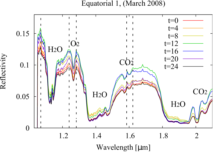
Figure 1.— Examples of NIR reflection spectra of the Earth observed by EPOXI in March of 2008 (Earth 1: equinox) (Livengood et al., 2011; Robinson et al., 2011) . Different lines represent different short exposures obtained at 2-hour intervals and labeled by the time $t$[hr] from the start of the observations on that date (see Figure 2). Three vertical dashed lines indicate the wavelength ranges that we adopt to compute the equivalent widths (H₂O: 1.07-1.24$\mu$m, O₂: 1.24$\mu$m-1.283$\mu$m, CO₂: 1.59-1.62$\mu$m).

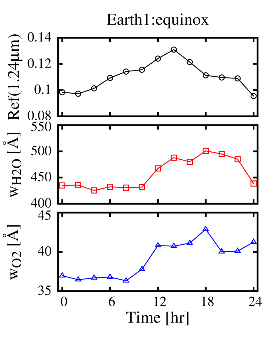
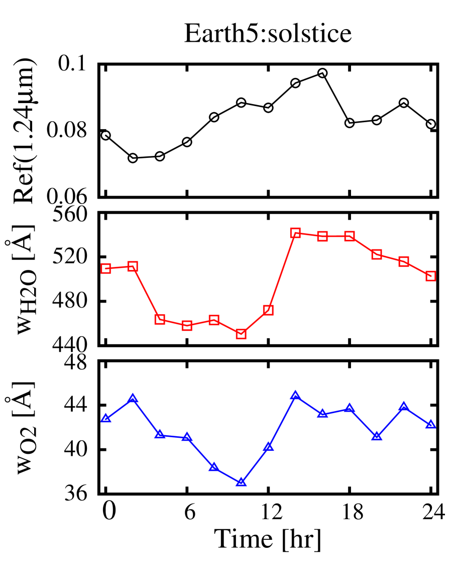
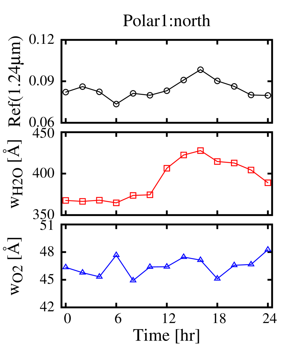
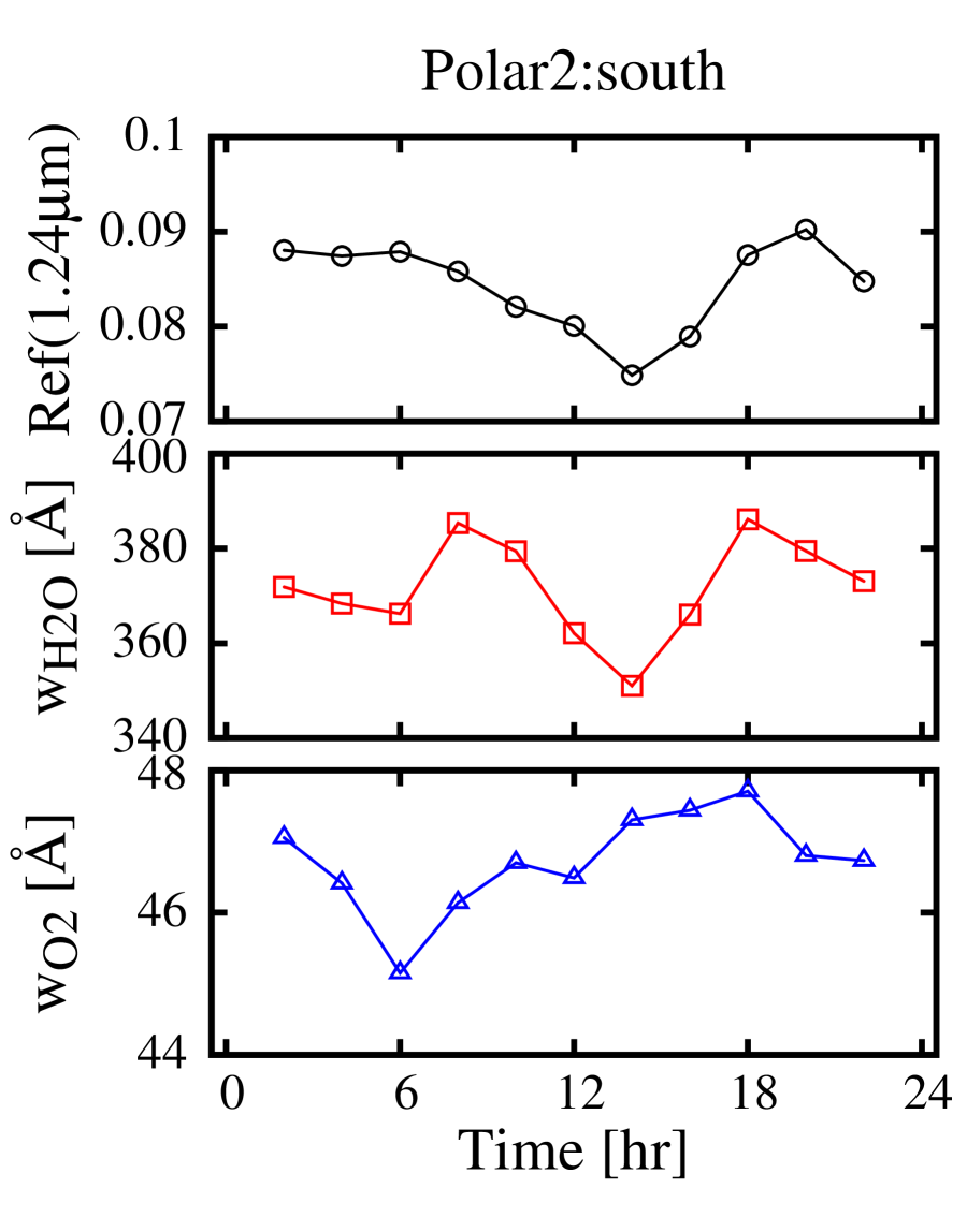
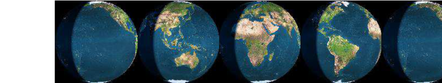
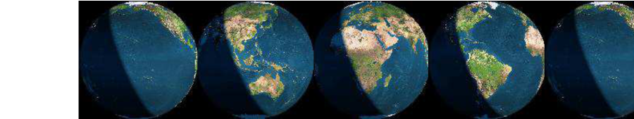
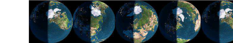
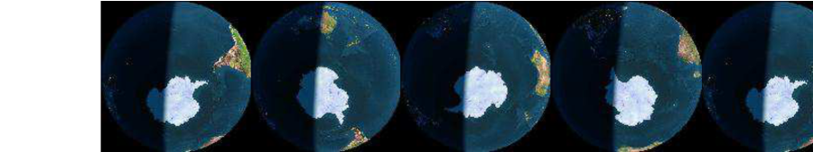
Figure 2.— Diurnal variations of continuum level (top), equivalent width of H₂O absorption centered at 1.13$\mu$m (middle), and that of O₂ centered at 1.27$\mu$m (bottom). Symbols indicate observed data points and the connecting lines are drawn only to guide the eyes. Snapshots at corresponding times were generated at http://www.fourmilab.ch/cgi-bin/uncgi/Earth are attached.

Table 1Diurnal Variation of Continuum Level, Equivalent Width of H₂O at 1.13$\mu$m and that of O₂ at 1.27$\mu$m.

	Reflectivity at 1.24$\mu$m		H2O at 1.13$\mu$m		O2 at 1.27$\mu$m
	ave.	(max-min)/ave	ave.[Å]	(max-min)/ave	ave.[Å]	(max-min)/ave
Earth1:equinox (Mar.2008)	0.111	32.1%	457	16.5%	39	16.8%
Earth5:solstice (Jun.2008)	0.084	30.6%	499	18.2%	42	18.7%
Polar1:north (Mar.2009)	0.084	29.5%	392	16.1%	46	7.2%
Polar2:south (Oct.2009)	0.084	18.2%	372	9.4%	47	5.5%

The EPOXI mission (Livengood et al., 2011) performed photometric and spectroscopic monitoring of the Earth and the Moon from space as a benchmark for future characterization of terrestrial exoplanets. A part of the observations were devoted to spectroscopy of the disk-integrated scattered light of the Earth over the wavelength of 1.10-4.54$\mu$m. These observations were carried out on 2008 March 18-19, 2008 June 4-5, 2009 March 27-28, and 2009 October 4-5, with 12 exposures every two hours of the day (integration time for each exposure is less than 2 sec). The sub-observer latitudes (the latitude of the intersection between the Earth’s surface and the line connecting the center of the Earth and the detector) are 1^∘.7 N, 0^∘.3 N, 61^∘.7 N, and $73^{\circ}$.8 S, respectively. Following Cowan et al. (2011), we henceforth refer to these 4 observations as Earth1:equinox, Earth5:solstice, Polar1:north, and Polar2:south.

Figure 1 displays the 1-2$\mu$m portion of the observed reflection spectra of the Earth in Earth1. The broad absorption features at 1.08-1.18, 1.30-1.53, and 1.75-1.99$\mu$m are mostly due to H₂O, and the narrower feature around 1.27$\mu$m is due to O₂ plus oxygen collision complexes O${}_{2}\cdot$O₂ and O${}_{2}\cdot$N₂ (Pallé et al., 2009, and references therein). Absorptions at 1.6$\mu$m and 2.0$\mu$m are signatures of CO₂ (e.g. Robinson et al., 2011).

We measure the equivalent widths of H₂O ($w_{\rm H_{2}O}$) and O₂ ($w_{\rm O_{2}}$) for each exposure. For $w_{\rm H_{2}O}$, we focus on the spectral features centered at $\sim 1.13\mu$m and consider the absorption from 1.07$\mu$m to 1.24$\mu$m. For $w_{\rm O_{2}}$, we use the spectral features centered at $\sim 1.27\mu$m and consider the absorption from 1.24$\mu$m to 1.283$\mu$m. In each case, the continuum line is assumed to connect the data points at both boundaries linearly. Additionally, we consider the variation of reflectivity at 1.24$\mu$m as a measure of the continuum level.

Figure 2 shows the diurnal fluctuations of $w_{\rm H_{2}O}$ and $w_{\rm O_{2}}$, as well as the variation of the reference continuum level (1.24 $\mu$m). Table 1 summarizes the average and the fractional variation amplitudes of continuum level, $w_{\rm H_{2}O}$ and $w_{\rm O_{2}}$. The variation amplitude defined by (maximum-minimum)/average is typically 5-20%. Figure 2 clearly indicates that the diurnal patterns of $w_{\rm H_{2}O}$ and $w_{\rm O_{2}}$ significantly differ from that of the continuum level which primarily traces the continental distribution on the Earth (see e.g. Cowan et al., 2009, 2011; Fujii et al., 2011). Although not shown here in detail, we also confirmed that absorption features of H₂O at other wavelengths (centered at $\sim 1.4\mu$m and $\sim 1.85\mu$m) exhibit variation patterns matching those at the 1.13$\mu$m band. For equatorial observations, the general trend that the depth is weaker in the first half of the day and becomes stronger in the second half is evident, and is shared by both H₂O and O₂. Referring to the snapshots shown in the bottom panels in Figure 2, the weaker absorption corresponds to the time when the Indonesia, a persistently cloudy region, dominates the field-of-view (see also Gómez-Leal et al., 2012). This already demonstrates the strong relation between the absorption bands and cloud cover. In the next subsection, we investigate this connection in more detail.

2.2. Correlation between diurnal variabilities and ocean/cloud parameters

As mentioned in Section 2.1, the variation pattern in Figure 2 is likely correlated with the extent and nature of cloud cover. In order to confirm the correlation between the absorption features and clouds, we collect daily global maps of atmospheric parameters for the corresponding days from Terra/MODIS Atmosphere Level 3 Product, which is available online. Each global map is derived on a pixel-to-pixel basis from the Remote Sensing data obtained with MOderate Resolution Imaging Spectroradiometer (MODIS) onboard the Earth Observing Satellites Terra and Aqua (Dorothy et al., 2006). Among the various parameters reported, we choose four which we suspect will influence the diurnal absorption variations strongly, including Atmospheric Water Vapor Mean, Cloud Top Pressure Mean ($P_{\rm ctp}$), Cloud Fraction Mean ($f_{\rm cld}$), and Cloud Optical Thickness Combined Mean ($\tau_{\rm cld}$). We further add the ocean fraction as a fifth parameter.

We compute the weighted average of each parameter for each EPOXI exposure. We adopt the geometric weight as ${\rm Max}\{\mu_{0}\mu_{1},0\}$, where $\mu_{0}$/$\mu_{1}$ denote the cosine between the normal direction of the surface and the direction toward the Sun/observer. We adopt this factor because each surface pixel would contribute to the total reflectivity with that weight if the scattering were isotropic (Lambert’s Law) (e.g. Lester et al., 1979); while this is not strictly the case, it is a reasonable approximation for these purposes.

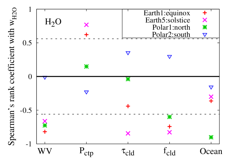
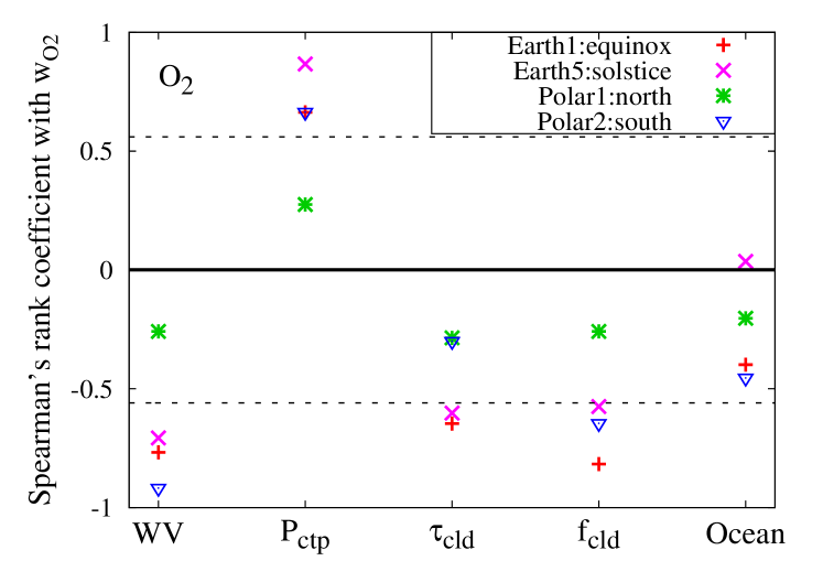
Figure 3.— Spearman’s rank correlation coefficient between absorption depth (left:H₂O, right:O₂) and Atmospheric Water Vapor (WV), Cloud Top Pressure ($P_{\rm ctp}$), Cloud Optical Thickness ($\tau_{\rm ftp}$), Cloud Cover Fraction ($f_{\rm cld}$), and Ocean Fraction (Ocean), respectively. Horizontal dotted lines show the significance level of 0.05 for 13 samples (# of exposures per observation).

Figure 3 displays Spearman’s rank correlation coefficients between absorption depths of H₂O (left) and O₂ (right) measured by EPOXI observation and parameters taken from MODIS. Spearman’s rank coefficient $r_{s}$ is calculated by converting each value $x_{i}$ ($i$:index for exposures in one series of observation) to the rank $X_{i}$. If $x_{j}$ is the $n$-th largest value of all possible values of $x_{i}$, the rank is defined as $X_{j}=n$. Then we calculate the correlation coefficient of the ranks of two different parameters $x_{i}$ and $y_{i}$ as

$$r_{s} = \frac{\displaystyle\sum_{i}(X_{i}-\bar{X})(Y_{i}-\bar{Y})}{\sqrt{\displaystyle\sum_{i}{(X_{i}-\bar{X})^{2}}}{\sqrt{\displaystyle\sum_{i}{(Y_{i}-\bar{Y})^{2}}}}},$$ (1)

$$\bar{X} = \sum_{i}X_{i},\qquad\bar{Y}=\sum_{i}Y_{i}.$$ (2)

Since the chosen parameters do not necessarily follow a gaussian distribution, we adopt Spearman’s rank correlation coefficients instead of Pearson’s correlation coefficients.

In most cases, the absorption depths are positively correlated with the cloud top pressure (or equivalently, anti-correlated with the cloud altitude), while anti-correlated with both cloud optical thickness and the cloud cover fraction. These trends are plausibly understood as follows: For cloud top pressure, the incident light is scattered at the altitude of the upper cloud layer without absorption by molecules in the atmosphere below the cloud. Since molecules are abundant in the lower atmosphere, the higher cloud altitude reduces the absorption depth more effectively. As for cloud optical thickness, thicker clouds scatter the incident light more completely and thus reduce absorptions below that layer. Additionally, the higher reflectivity of the thicker cloud increases the contribution of the region to the disk-integrated spectra. Similarly, the absorption depths become weaker as the cloud cover fraction increases.

Although more weakly, the absorption depths appear to be slightly anti-correlated with the ocean fraction. The lower reflectivity of ocean reduces the absorption depths of the disk-integrated spectra.

We should emphasize here, however, that the above interpretation requires some caution because the five parameters we adopted are not necessarily independent. In the equatorial region, for instance, there exists a positive correlation between cloud optical thickness and cloud top altitude. There is also generally positive correlation between cloud cover and atmospheric water vapor, likely leading to the counter-intuitive anti-correlation between the atmospheric water vapor and the absorption depths.

Figure 3 also shows that the correlation of the H₂O band with clouds varies more significantly than that of O₂, depending on the location of the sub-observer’s latitude. In particular, the correlation of H₂O for Polar2 observation even changes its sign compared to the other three cases. This is not the case for O₂. We will discuss this behavior in detail in Section 4.

3. A Simple Opaque Cloud Model

In the previous section, we discussed the influence of clouds on absorption features by considering the correlation between the absorption depths and individual cloud/surface parameter. In this section, we try to interpret the observed variation in absorption depths more quantitatively. For that purpose, we consider a simple opaque cloud model (see also e.g. Harrison & Coombes, 1988), which assumes that the cloud cover totally blocks the influence of the lower atmosphere and that the incident light is completely scattered at the cloud top.

3.1. Model Description

The equivalent width of an atmospheric absorption band in the disk-integrated scattered light of the planet can be expressed as

$$w_{\rm model}=\int_{\lambda_{0}-\Delta\lambda}^{\lambda_{0}+\Delta\lambda}d\lambda~{}\frac{\int_{S_{\rm IV}}c_{\lambda}(\theta,\phi)\left[1-e^{-\tau_{\lambda}}\right]g(\theta,\phi)\;d\Omega}{\int_{S_{\rm IV}}c_{\lambda}(\theta,\phi)g(\theta,\phi)\;d\Omega},$$ (3)

$$d\Omega\equiv\sin\theta d\theta d\phi,\qquad g(\theta,\phi)\equiv\mu_{0}\mu_{1},$$ (4)

where $(\theta,\phi)$ represents the polar-coordinate of the surface point on the planet, $\mu_{0}=\mu_{0}(\theta,\phi)$ and $\mu_{1}=\mu_{1}(\theta,\phi)$ are the directional cosines between the normal direction of the surface point and the direction toward the Sun and the observer, respectively. The wavelength-dependent continuum level (i.e., reflectivity) and optical depth are denoted by $c_{\lambda}(\theta,\phi)$ and $\tau_{\lambda}$. The interval of integration over $\lambda$ is centered at the center of the absorption band, $\lambda_{0}$. The integral over solid angle of planetary surface is performed over the illuminated and visible portion, $S_{\rm IV}$. The above expression is based on the approximations that 1) the lower boundary scatters the light according to the Lambert Law, i.e. the scattered intensity is independent of the emergent direction, and 2) scattering by the atmosphere is negligible.

We further neglect the wavelength-dependence of the continuum level, and assume that the wavelength dependence of $c_{\lambda}(\theta,\phi)$ can be factored out, i.e., $c_{\lambda}(\theta,\phi)=h(\lambda)c(\theta,\phi)$ with $h(\lambda)$ being a function of wavelength alone. Then, equation (3) may be approximated as

$$w_{\rm model} = \frac{\int_{S_{\rm IV}}c(\theta,\phi)W(N;\theta,\phi)g(\theta,\phi)d\Omega}{\int_{S_{\rm IV}}c(\theta,\phi)g(\theta,\phi)d\Omega},$$ (5)

$$W(N;\theta,\phi) \equiv \int d\lambda\;\left(1-\exp\{-\tau_{\lambda}(N;\theta,\phi)\}\right),$$ (6)

$$\tau_{\lambda}(N;\theta,\phi) = \int_{z_{0}}^{\infty}n(z)\sigma_{\lambda}\left(\frac{1}{\mu_{0}}+\frac{1}{\mu_{1}}\right)dz$$ (7)

$$\sim \left(\frac{1}{\mu_{0}}+\frac{1}{\mu_{1}}\right)\frac{\int n(z)dz\cdot\int n_{0}(z)\sigma_{\lambda}dz}{\int n_{0}(z)dz}$$

$$= \frac{N_{\rm eff}}{N_{0}}\tau_{\lambda,0}\;,$$

$$N_{\rm eff} \equiv \left(\frac{1}{\mu_{0}}+\frac{1}{\mu_{1}}\right)\int_{z_{0}}^{\infty}n(z)dz\;,$$ (8)

where $W(N;\theta,\phi)$ is the equivalent width at each surface patch, $\sigma_{\lambda}$ is the absorption coefficient, $N_{0}$ is the total column density of molecules under the canonical atmospheric model, $N_{\rm eff}$ is the effective column density obtained by integrating $n(z)$ along the optical path from the top of atmosphere down to the boundary at altitude $z=z_{0}$, and $\tau_{\lambda,0}$ is the absorption depth of the canonical model. Equation (7) is only approximately valid because in reality the absorption coefficient $\sigma_{\lambda}$ depends on the T-P profile of atmosphere. Nevertheless, we employ this approximation for the sake of simplicity.

In practice, we divide the planetary surface into $2^{\circ}\times 2^{\circ}$ pixels, and treat the cloudless and cloudy portions in each pixel separately for convenience, as described below. Then, equation (5) is discretized as

$$w_{\rm model}=\frac{\displaystyle\sum_{i}\left\{(1-f_{\rm cld}^{i})\,W_{\rm nocld}^{i}c_{\rm nocld}^{i}+f_{\rm cld}^{i}\,W_{\rm cld}^{i}c_{\rm cld}^{i}\right\}g^{i}\delta\Omega^{i}}{\displaystyle\sum_{i}\left\{(1-f_{\rm cld}^{i})\,c_{\rm nocld}^{i}+f_{\rm cld}^{i}\,c_{\rm cld}^{i}\right\}g^{i}\delta\Omega^{i}},$$ (9)

where $i$ is the index for the surface pixels, $f_{\rm cld}$ is the cloud cover fraction, and the suffix _nocld/_cld indicates the value at the cloudless/cloudy portion. The position-dependent parameters in equation (9) are determined on the basis of daily global maps which are extracted from the same MODIS data product used in Section 2.2. For instance, the value for $f_{\rm cld}$ is adopted from Cloud Fraction Mean. Input data for other parameters are described below.

The effective column density $N_{\rm eff}$ of H₂O at each patch is determined by Atmospheric Water Vapor Mean ($w$) and Cloud Top Pressure Mean ($P_{\rm ctp}$) as well as the geometric factors $\mu_{0}$ and $\mu_{1}$. For the cloudless portion, $N_{\rm eff}$ is identical to $(1/\mu_{0}+1/\mu_{1})w$ because we can safely set $z_{0}=0$. For cloudy portions of a pixel, however, we need to define the boundary height $z_{0}$ in equation (7) that is essentially the layer below which the the molecule in question does not influence the emergent spectra. In the present opaque cloud model, we assume that the synthetic absorption depth is completely unaffected by the atmosphere below the cloud top altitude $z_{\rm ctp}$, and thus set $z_{0}=z_{\rm ctp}$. According to this opaque cloud assumption, $N$ is determined once the vertical profile of water vapor and the altitude of the cloud top layer are given. In what follows, we simply assume that the vertical profile of water vapor is proportional to that of the US Standard Model, and determine the proportionality coefficient so that the total column density matches the value of $w$. The altitude of the cloud top layer is derived from $P_{\rm ctp}$ assuming the US Standard Temperature-Pressure (T-P) profile. The total column density $N_{\rm eff}$ for O₂ is estimated in the same way except that we neglect the horizontal inhomogeneity, and determine it only from $P_{\rm ctp}$ and the geometric factor.

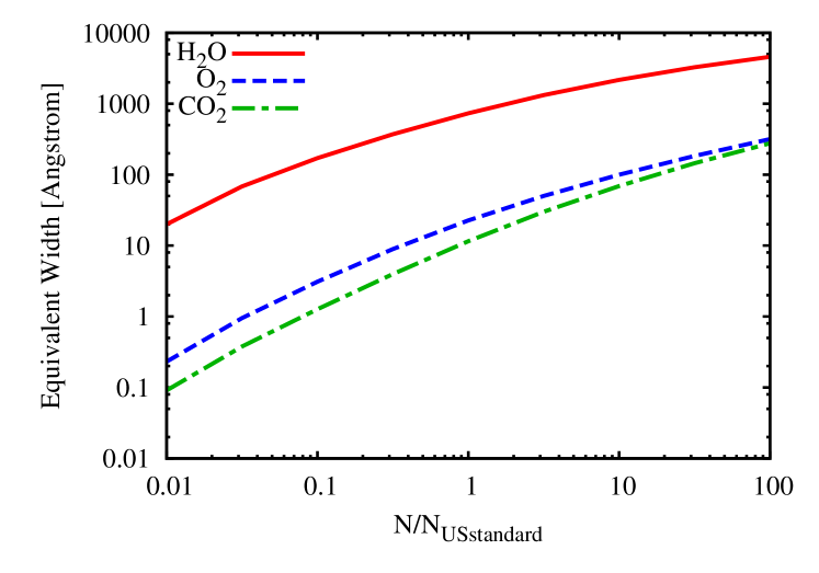
Figure 4.— Curve of growth for the equivalent width of the water vapor absorption band at 1.13$\mu$m-1.24$\mu$m, oxygen at 1.24$\mu$m-1.283$\mu$m, and carbon dioxide at 1588$\mu$m-1.622$\mu$m calculated by lbl2od with GEISA 2011 database under the no-cloud condition with surface albedo 0.3.

The remaining task is to compute the equivalent width $W$ as a function of the effective column density. For this purpose, we compute line-by-line optical depths $\tau_{\lambda,0}$ under the US Standard Atmosphere with the GEISA 2011 molecule spectroscopic database and the public code lbl2od. Then we calculate $\int_{\lambda_{0}-\Delta\lambda}^{\lambda_{0}+\Delta\lambda}e^{-\kappa\tau_{\lambda,0}}d\lambda$ with varying $\kappa$. Figure 4 shows the resultant curve of growth of the equivalent widths of H₂O measured at $1.06-1.24\mu$m, O₂ at $1.235-1.310\mu$m as well as CO₂ at $1.560-1.630\mu m$ used in Appendix A. Based on these calculations, the normalized effective column density of each patch, $N^{i}_{\rm eff}/N_{\rm USstandard}$, is translated into the equivalent width $W^{i}$ by equating $N^{i}_{\rm eff}/N_{\rm USstandard}$ to $\kappa$ in Figure 4.

Finally, the continuum level $c$ in equation (9) is estimated using the 2-stream approximation (e.g. Liou, 1980). We consider a non-absorbing atmosphere with optical thickness $\tau_{\rm cld}$ and asymmetry factor $\beta$. Denoting the reflectivity at the surface by $r_{g}$, the net reflectivity at the top of the atmosphere is:

$$c(\tau_{\rm cld})=\alpha\left[1-\frac{1-r_{g}}{1+(\sqrt{3}/2)(1-r_{g})(1-\beta)\tau_{\rm cld}}\right],$$ (10)

where we adopt the optical thickness of the cloud (Cloud Optical Thickness Combined Mean) for $\tau_{\rm cld}$. The typical value for $\beta$ of Earth’s clouds at the relevant wavelengths is $\beta=0.85$ (e.g. Liou, 1980). The overall scaling factor $\alpha$ is introduced here to empirically incorporate the anisotropic scattering due to the bulk cloud cover. We determine the value of $\alpha$ by hand so as to match the disk-averaged continuum level to the observed data.

According to the procedures described above, we compute $W^{i}$ and $c^{i}$ at each pixel, and then obtain the predicted absorption depth in the disk-averaged spectra of the Earth from equation (9). The model prediction is compared with the EPOXI data in Section 3.2.

3.2. Comparison of the opaque cloud model and the EPOXI Data

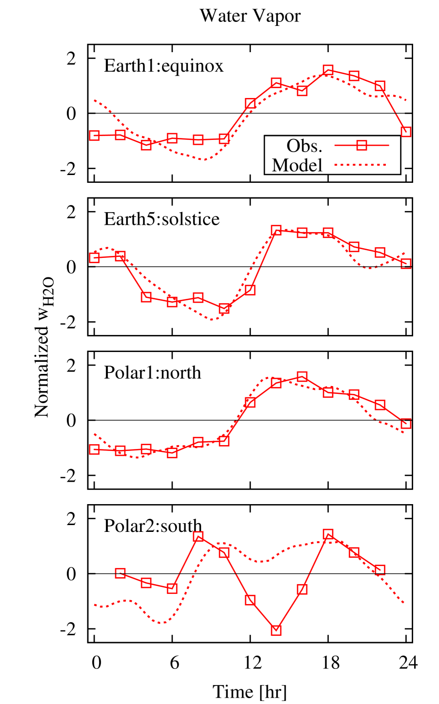
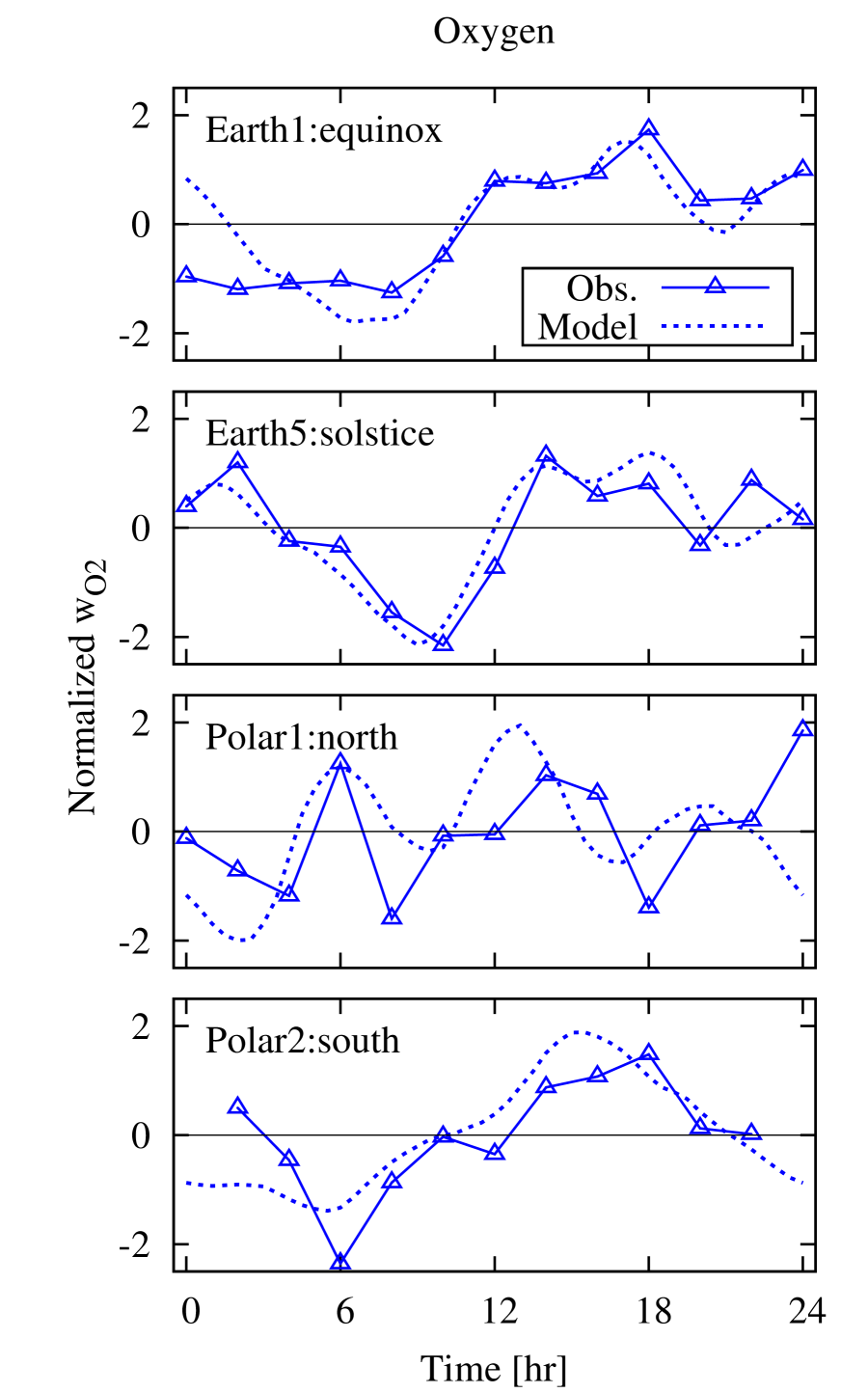
Figure 5.— Comparison between the EPOXI data (symbols) and simulations (dashed lines) in terms of continuum level measured at 1.24$\mu$m (left), water vapor absorption (middle), and oxygen absorption (right).

Figure 5 compares the EPOXI data (symbols) to our model predictions (dotted lines). The left, middle and right panels correspond to the disk-integrated continuum level, H₂O absorption, and O₂ absorption, respectively. The anisotropic parameter for bulk cloud scattering $\alpha$ in equation (10) is determined so that the disk-averaged continuum level matches the observed value (Table 2).

Table 2Normalization Parameters and Comparison in Daily Average and Standard Deviation between Simulations and Observations.

	Earth1	Earth5	Polar1	Polar2
$\alpha$	0.61	0.64	0.73	0.79
$\bar{w}_{\rm H2O,model}/\bar{w}_{\rm H2O,obs}$	0.85	0.87	0.88	0.88
$\bar{w}_{\rm O2,model}/\bar{w}_{\rm O2,obs}$	0.65	0.66	0.64	0.63
$\sigma_{\rm H2O,model}/\sigma_{\rm H2O,obs}$	1.32	1.73	0.70	0.92
$\sigma_{\rm O2,model}/\sigma_{\rm O2,obs}$	0.57	0.77	0.61	0.88

We first consider the comparison between the simulation and the observation in terms of the daily average, $\bar{w}$, and the standard deviation, $\bar{\sigma}$. Table 2 summarizes the ratio of the daily average of the simulated $\bar{w}_{\rm model}$, to the observed one, $\bar{w}_{\rm obs}$, $\bar{w}_{\rm model}/\bar{w}_{\rm obs}$, and that of standard deviation $\bar{\sigma}_{\rm model}/\bar{\sigma}_{\rm obs}$. The daily simulation average typically results in a 10-15% underestimation for H₂O and 35% underestimation for O₂. The underestimation is likely due to our “opaque cloud” assumption which tends to diminish the absorption depth; in reality cloud cover does not completely prevent the light from going through the lower atmosphere. Uncertainty can also come from the difficulty in determining the continuum level because the absorption bands we are considering are surrounded by other absorption features.

The variation pattern, which is of our primary interest in this paper, is less sensitive to those uncertainties. The absorption depths normalized so that the daily average is 0 and the standard deviation is unity are exhibited in the middle and right panels of Figure 5. In most cases, the overall variation patterns of both H₂O and O₂ are well reproduced by our opaque cloud model. In particular, the equatorial data (Earth1, Earth5) exhibit striking agreement with the model predictions. For polar observations, the agreement is somewhat degraded, especially for H₂O variations in the Polar2 data. This may be partly ascribed to the fact that there is a slight mismatch between the time of the EPOXI observation and that of the input atmospheric data of our simulation; the local time of MODIS observation is 10:30am for Terra and 12:10pm for Aqua, while the disk-integrated spectra observed by EPOXI reflects the information of slices with different local times. In addition, the assumed vertical profile for H₂O (the US standard atmosphere) is not expected to be as accurate for the equatorial/polar regions. While our model is admittedly rough in this regard, it is encouraging that such a simple model reproduces the general trends and features observed by EPOXI fairly well.

4. Different Variation Patterns of H₂O and O₂ Absorption Depths

We now focus on the intriguing differences in behavior between H₂O and O₂. In the Earth1 and Earth5 data, for instance, note the small deviation of the H₂O pattern from the O₂ pattern, including the sharper bump of $w_{\rm O2}$ at $t=18$[hr] than $w_{\rm H2O}$. Polar1 observations show the variation of $w_{\rm H2O}$ rising at $11\leq t{\rm[hr]}\leq 19$, which is not present in the variation of $w_{\rm O2}$. In addition, only $w_{\rm O2}$ has a local peak at $t=6$. Significantly and reassuringly, these divergences are reproduced by our simulations, which allows us to isolate the origin of this difference.

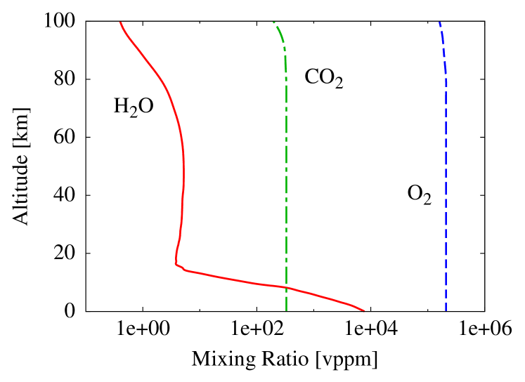
Figure 6.— Vertical profiles of H₂O (red solid) and O₂ (blue dashed) taken from US standard model.

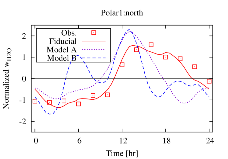
Figure 7.— Comparison in H₂O band variation between observation and simulations with different assumption for water vapor distribution. Model A adopts the water vapor vertical profile of US standard model but neglect the horizontal inhomogeneity. Model B assumes constant mixing ratio in the troposphere as is the case for O₂.

Let us discuss the possible causes of the different diurnal pattern of H₂O and O₂ bands. Given that the absorption depth in our model is directly linked to the total number of molecules above the cloud layers, the different behaviors of H₂O and O₂ exhibited in Figure 5 can only be ascribed to the differences in their column number density distribution in the planetary atmosphere.

In the case of the Earth, the distribution of water vapor differs from that of O₂ in at least two ways. Firstly, the total column density of atmospheric water vapor is, unlike O₂, a strong function of latitude (highly concentrated in the equatorial region) with additional local/temporal fluctuations. Secondly, the vertical profile of water vapor mixing ratio typically decreases as a function of altitude due to condensation, in contrast to the constant mixing ratio (volume fraction of the molecule) of O₂ in the troposphere (Figure 6).

In order to evaluate these effects quantitatively, we run simulations of H₂O band variation with different assumptions for its atmospheric distribution. We consider two model distributions in addition to our fiducial model described in Section 3.1: Model A adopts the water vapor vertical profile of the US Standard Model everywhere, and thus the mixing ratio decreases with altitude (red solid line in Figure 6). Model B instead assumes a constant mixing ratio of H₂O in the troposphere as is the case for O₂ (blue dashed line in Figure 6). Both Models A and B neglect the inhomogeneity of water vapor over the surface of the planet.

These three simulations and observations in the Polar1:north case are plotted in Figure 7. The observed variation of H₂O agrees well with fiducial model, while the other two models that neglect the horizontal or surface inhomogeneity and/or peculiar vertical profiles fail to match the observed data. We also note that the Model B (blue line in Figure 7) prediction of $w_{\rm H_{2}O}$ is very close to that of the simulation for O₂ in the Polar1 case (solid line in the third panel of O₂ in Figure 5). This indeed implies that that the differences in variation patterns basically reflect their differing spatial distributions in the atmosphere.

Both of the above-mentioned properties of water vapor distribution are consequences of the coexistence of multiple phases of water on Earth. The horizontal inhomogeneity of water vapor originates from the temperature gradient over the surface (since the vaporization rate is basically determined by the surface temperature) and/or the inhomogeneous distribution of liquid/solid reservoirs on the surface. The water vapor distribution is not mixed well since the mean residence time (MRT) of atmospheric H₂O ($\sim$10 days) is much shorter than the time scale of the vertical and global mixing times of the atmosphere (both $\sim$ 1 year). In contrast, the MRT of O₂ is $\sim$4000 years, thus insuring that O₂ is well mixed and only very slowly changing, if at all.

The short MRT of water vapor implies that there is a non-negligible flux of H₂O into/out of atmosphere and the existence of a substantial water reservoir (compared to the abundance in the atmosphere), such as the oceans on the Earth. Figure 7 also indicates that the difference in the vertical profile alone may lead to differences in the variation of absorption bands, but this is also related to the condensation of water in the atmosphere. In either case, the deviation of absorption features of H₂O from the well-mixed gas like O₂ may serve as an indicator of phases transitions happening in the atmosphere or on the surface of a planet. This signature of the Earth’s “water cycle” could be an observable indicator of a similar climate on a terrestrial exoplanet.

5. Summary and Discussion

In this paper we examined the diurnal variability of the absorption depths of the two important molecules, H₂O and O₂, in the disk-integrated spectra of the Earth. We analyzed the H₂O band centered at $\sim 1.13\mu$m and O₂ band centered at $\sim 1.27\mu$m observed by EPOXI and found that these absorption bands show diurnal variations correlated with uneven cloud cover. A simple opaque cloud model, which assumes that the cloud completely blocks the atmospheric signatures below the cloud top layer, is able to reproduce the basic variation patterns of the H₂O and O₂ bands using pixel-level cloud data obtained with Earth Observing Satellite. Thus we conclude that the non-uniform cloud cover distribution dominates the observed diurnal variations of those molecular absorption depths.

However, we also found that the diurnal variability patterns of H₂O and O₂ bands are not identical, and the differences originate from the inhomogeneous distribution of water vapor in the atmosphere. The variability pattern of O₂ is basically explained by the the cloud cover distribution because it is well mixed in the troposphere of the Earth. In contrast, the variability pattern of H₂O is well reproduced only with additional information on the vertical profile and spatial inhomogeneity of atmospheric water vapor as a model input. The nature of the water vapor distribution in the atmosphere is linked to the fact that H₂O circulates in the planetary surface layer changing its phase among water vapor, liquid water (ocean/lake/pond/river) and/or water ice. Therefore, different behavior in the variability patterns of O₂ and H₂O absorptions may carry information on the inhomogeneous phase distribution of H₂O in the surface layer.

Our study of the Earth demonstrates the possible role of the variability of absorption bands in characterizing the surface environments of Earth-analogs. If future instruments eventually succeed in detecting scattered light from such exoplanets, their time-resolved measurements of the absorption bands will reveal the uneven cloud cover and/or inhomogeneous spatial distribution of atmospheric constituents. Our current results suggest that the comparison in variation pattern between presumably well-mixed gases (such as O₂) and H₂O may indicate frequent phase transitions of water in the surface layer and thus serve as a probe of habitability, in a complementary fashion to the direct detection of liquid water (e.g. Williams & Gaidos, 2008; Oakley & Cash, 2009; Robinson et al., 2010; Zugger et al., 2010) and the search for other potential biosignatures (e.g. Kaltenegger et al., 2010; Kawahara et al., 2012).

While we focused on absorption bands in the NIR range where the EPOXI data are available, it is natural to expect that other bands also exhibit similar variation patterns at wavelengths dominated by scattering of the primary star’s light, rather than planetary thermal emission. In the visible range, there are O₂ bands at 0.69$\mu$m (equivalent width $\sim$13.5Å) and at 0.76$\mu$m (equivalent width $\sim$47.8Å) (e.g. Pallé et al., 2009) as well as several H₂O bands.

Inhomogeneity of an atmospheric constituent becomes appreciable when its MRT is short compared to the time-scale of the atmosphere mixing. This is equivalent to there being a substantial flux of the molecular species in question between the atmosphere and some surface reservoir, i.e., substantial compared to the total amount residing in the atmosphere. Besides vaporization, photochemical production (e.g. O₃) or biotic production (e.g. N₂O, CH₄) could lead to such a situation. If sufficiently accurate data become available in the future, we may be able to interpret implied inhomogeneous distributions in terms of those or other specific mechanisms.

Appendix A Variation of CO₂

We also examine the variability of CO₂, another absorption feature imprinted in the observed spectra. Absorption bands of CO₂ exist around 1.6$\mu$m and 2$\mu$m (Figure 1). These CO₂ bands override the wings of H₂O absorption, making it harder to determine the continuum level. We pick up the absorption band at 1.59-1.62$\mu$m, which is likely to be least affected by H₂O absorption. The peak-to-throat variation amplitude of four observations are 5-20%(Table 3), on the same level of O₂ and H₂O.

Figure 8 shows the diurnal variation patterns of CO₂ band at 1.59-1.62$\mu$m extracted from EPOXI data as well as those of our simulation following the same procedure as H₂O/O₂ and assuming the uniform distribution (the assumed growth curve of this band is displayed in Figure 4). The normalization factors are summarized in Table 4. We see the clear similarity in variation patterns to O₂ rather than H₂O. For instance, the clearer bumps at $t=18$ of Earth1 and Earth5 observations and the gradient in Polar2 observation. This result is consistent with our discussion in Section 4, since the MRT of CO₂ is 3-5 years and slightly longer than the tropospheric mixing timescale. The behavior of Polar1 is less conclusive and the observation does not match the simulation so well . Although we do not identify the cause, it might be related to some level of inhomogeneity of CO₂ due to the intermediate MRT.

Table 3Diurnal Variation of Continuum Level, Equivalent Width of CO₂ at 1.6$\mu$m.

	CO2 at 1.6$\mu$m
	ave.[Å]	(max-min)/ave
Earth1:equinox (Mar.2008)	12.1	80.1%
Earth5:solstice (Jun.2008)	17.8	17.4%
Polar1:north (Mar.2009)	17.4	11.3%
Polar2:south (Oct.2009)	17.9	5.4%

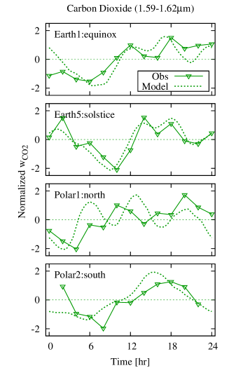
Figure 8.— Diurnal Variations of CO₂ absorption bands around 1.59-1.62 $\mu$m. EPOXI data (symbols) and simulations (dashed lines) are compared.

Table 4Normalization Parameters and Comparison in Daily Average and Standard Deviation between Simulations and Observations.

	Earth1	Earth5	Polar1	Polar2
$\bar{w}_{\rm CO2,model}/\bar{w}_{\rm CO2,obs}$	1.14	0.85	0.95	0.90
$\sigma_{\rm CO2,model}/\sigma_{\rm CO2,obs}$	0.23	1.23	0.74	1.75

References

- Abe et al. (2011) Abe, Y., Abe-Ouchi, A., Sleep, N. H., & Zahnle, K. J. 2011, Astrobiology, 11, 443
- Blake & Shaw (2011) Blake, C. H., & Shaw, M. M. 2011, PASP, 123, 1302
- Cowan et al. (2009) Cowan, N. B., et al. 2009, ApJ, 700, 915
- Cowan et al. (2011) Cowan, N. B., et al. 2011, ApJ, 731, 76
- Dorothy et al. (2006) Dorothy, K. H., George A. Riggs, A. G., & Salomonson, V. V. 2006, updated daily, MODIS/Terra Aerosol Cloud Water Vapor Ozone Daily L3 Global 1Deg CMG, Boulder, Colorado USA: National Snow and Ice Data Center. Digital media.
- Ford et al. (2001) Ford, E. B., Seager, S., & Turner, E. L. 2001, Nature, 412, 885
- Fujii & Kawahara (2012) Fujii, Y., & Kawahara, H. 2012, arXiv:1204.3504
- Fujii et al. (2011) Fujii, Y., Kawahara, H., Suto, Y., Fukuda, S., Nakajima, T., Livengood, T. A., & Turner, E. L. 2011, ApJ, 738, 184
- Fujii et al. (2010) Fujii, Y., Kawahara, H., Suto, Y., Taruya, A., Fukuda, S., Nakajima, T., & Turner, E. L. 2010, ApJ, 715, 866
- Gómez-Leal et al. (2012) Gómez-Leal, I., Pallé, E., & Selsis, F. 2012, ApJ, 752, 28
- Harrison & Coombes (1988) Harrison, A. W., & Coombes, C. A. 1988, Solar Energy, 41, 387
- Kaltenegger et al. (2010) Kaltenegger, L., et al. 2010, Astrobiology, 10, 89
- Kawahara & Fujii (2010) Kawahara, H., & Fujii, Y. 2010, ApJ, 720, 1333
- Kawahara & Fujii (2011) Kawahara, H., & Fujii, Y. 2011, ApJ, 739, L62
- Kawahara et al. (2012) Kawahara, H., Matsuo, T., Takami, M., Fujii, Y., Kotani, T., Murakami, N., Tamura, M., & Guyon, O. 2012, arXiv:1206.0558
- Lester et al. (1979) Lester, T. P., McCall, M. L., & Tatum, J. B. 1979, JRASC, 73, 233
- Levine et al. (2009) Levine, M., et al. 2009, ArXiv e-prints
- Liou (1980) Liou, K. N. 1980, New York, NY (USA): Academic Press
- Livengood et al. (2011) Livengood, T. A., et al. 2011, Astrobiology, 11, 907
- Matsuo & Tamura (2010) Matsuo, T., & Tamura, M. 2010, in the Society of Photo-Optical Instrumentation Engineers (SPIE) Conference, Vol. 7735, Society of Photo-Optical Instrumentation Engineers (SPIE) Conference Series
- Mayer & Kylling (2005) Mayer, B., & Kylling, A. 2005, Atmospheric Chemistry & Physics, 5, 1855
- Oakley & Cash (2009) Oakley, P. H. H., & Cash, W. 2009, ApJ, 700, 1428
- Pallé et al. (2009) Pallé, E., Zapatero Osorio, M. R., Barrena, R., Montañés-Rodríguez, P., & Martín, E. L. 2009, Nature, 459, 814
- Palmer & Williams (1974) Palmer, K. F., & Williams, D. 1974, Journal of the Optical Society of America (1917-1983), 64, 1107
- Robinson et al. (2010) Robinson, T. D., Meadows, V. S., & Crisp, D. 2010, ApJ, 721, L67
- Robinson et al. (2011) Robinson, T. D., et al. 2011, Astrobiology, 11, 393
- Sanromá & Pallé (2012) Sanromá, E., & Pallé, E. 2012, ApJ, 744, 188
- Savransky et al. (2010) Savransky, D., Spergel, D. N., Kasdin, N. J., Cady, E. J., Lisman, P. D., Pravdo, S. H., Shaklan, S. B., & Fujii, Y. 2010, in the Society of Photo-Optical Instrumentation Engineers (SPIE) Conference, Vol. 7731, Society of Photo-Optical Instrumentation Engineers (SPIE) Conference Series
- Tinetti et al. (2006a) Tinetti, G., Meadows, V. S., Crisp, D., Fong, W., Fishbein, E., Turnbull, M., & Bibring, J. 2006a, Astrobiology, 6, 34
- Tinetti et al. (2006b) Tinetti, G., Meadows, V. S., Crisp, D., Kiang, N. Y., Kahn, B. H., Fishbein, E., Velusamy, T., & Turnbull, M. 2006b, Astrobiology, 6, 881
- Williams & Gaidos (2008) Williams, D. M., & Gaidos, E. 2008, Icarus, 195, 927
- Zugger et al. (2010) Zugger, M. E., Kasting, J. F., Williams, D. M., Kane, T. J., & Philbrick, C. R. 2010, ApJ, 723, 1168