Current in coherent quantum systems connected to mesoscopic Fermi reservoirs

Abstract

We study particle current in a recently proposed model for coherent quantum transport. In this model a system connected to mesoscopic Fermi reservoirs (meso-reservoir) is driven out of equilibrium by the action of super reservoirs thermalized to prescribed temperatures and chemical potentials by a simple dissipative mechanism described by the Lindblad equation. We compare exact (numerical) results with theoretical expectations based on the Landauer formula.

I Introduction

Particle current trough a coherent mesoscopic conductor connected at its left and right hand side to reservoirs is usually described in the non-interacting case by a formula, due to Landauer, based on the following physical picture: Electrons in the left (right) reservoir which are Fermi distributed with chemical potential $\mu_{L}$ ($\mu_{R}$) and inverse temperature $\beta_{L}$ ($\beta_{R}$) can come close to the conductor and feed a scattering state that can transmit it to the right (left) reservoir. All possible dissipative processes such as thermalization occur in the reservoirs while the system formed by the conductor and the leads is assumed to be coherent. The probability of being transmitted is a property of the conductor connected to the leads which is treated as a scattering system. In this picture, the probability that an outgoing electron comes back to the conductor before being thermalized is neglected, the contact is said to be reflectionless. This description of the non-equilibrium steady state (NESS) current through a finite system has been rigorously proved in some particular limiting situations needref , such as infinite reservoirs, but several difficulties prevail the understanding of non-equilibrium states in general and the description of current in more general situations, for instance in the case of interacting particles. Two frameworks are usually considered to study these open quantum systems: one deals with the properties of the state of the total (infinite) system Rue00 ; tasaki where reservoirs are explicitly considered as part of the system. The other is based on the master equation of the reduced density operator, obtained by tracing out the reservoirs’ degrees of freedom and is better suited to be applied to different systems and to compute explicitly some averaged NESS properties, at the price of several approximations such as e.g., Born-Markov (see e.g. Wichterich07 ).

In this paper we explore particle current in a model where we mimic the leads that connect the reservoirs with the system, as a finite non-interacting system with a finite number of levels (which we call meso-reservoir). The reservoirs (called here super-reservoirs) are modeled by local Lindblad operators representing the effect that a Markovian macroscopic reservoirs have over the meso-reservoirs. In Sec. II we introduce the model and briefly review the method we use to solve it. In Sec. III we analyze the particle current operator and indicate the quantities that should be computed for a full description of the current. In Sec. III.1 we briefly present the Landauer formula that is expected to apply in some appropriate limits to our model and in Sec. III.2 we analyze the numerical results we obtained with our model and compare them with the current predicted by the Landauer formula, validating the applicability of our model but also going beyond by computing the full probability distribution function (PDF) of the current. In Sec. IV we present some conclusions and discuss interesting perspectives of our study.

II Description of the model

We consider a one-dimensional quantum chain of spinless fermions coupled at its boundaries to meso-reservoirs comprising a finite number of spinless fermions with wave number $k$ ($k\in\{1,\ldots,K\}$). The Hamiltonian of the total system can be written as $H=H_{S}+H_{L}+H_{R}+V$, where

$$H_{S}=-\sum_{j=1}^{N-1}\Big{(}t_{j}c_{j}^{\dagger}c_{j+1}+({\rm h.c.})\Big{)}+\sum_{j=1}^{N}Uc_{j}^{\dagger}c_{j}$$ (1)

is the Hamiltonian of the chain with $\{t_{j}\}$ the nearest neighbor hopping, $U$ the onsite potential and $c_{j},c_{j}^{\dagger}$ the annihilation/creation operator for the spinless fermions on the site $j$ of the chain (conductor). The chain interacts through the term

$$V=\sum_{k=1}^{K}\left(v^{L}_{k}a_{kL}^{\dagger}c_{1}+v^{R}_{k}a_{kR}^{\dagger}c_{n}\right)+({\rm h.c.}),$$ (2)

with the meso-reservoirs $H_{\alpha}=\sum_{k=1}^{K}\varepsilon_{k}a_{k\alpha}^{\dagger}a_{k\alpha}$. Here $\alpha\!=\!\{L,R\}$ denotes the left and right meso-reservoir. They share the same spectrum with a constant density of states $\theta_{0}$ in the band $[E_{\rm min},E_{\rm max}]$ described by $\varepsilon_{k}\equiv\theta_{0}(k-k_{0})$ and $a_{k,\alpha},a^{\dagger}_{k,\alpha}$ are annihilation/creation operator of the left and right meso-reservoirs. The system is coupled to the leads only at the extreme sites of the chain with coupling strength $v_{k}^{\alpha}$ that we choose $k$-independent  $v_{k}^{\alpha}=v_{\alpha}$.

We assume that the density matrix of the chain - meso-reservoirs system evolves according to the many-body Lindblad equation

$$\frac{{\rm d}}{{\rm d}t}\rho = -i[H,\rho]+\sum_{k,\alpha,m}\left(2L_{k,\alpha,m}\rho L_{k,\alpha,m}^{\dagger}-\{L_{k,\alpha,m}^{\dagger}L_{k,\alpha,m},\rho\}\right),$$ (3)

where $m\in\{1,2\}$ and $L_{k,\alpha,1}=\sqrt{\gamma(1-F_{\alpha}(\varepsilon_{k}))}a_{k\alpha},\quad L_{k,\alpha,2}=\sqrt{\gamma F_{\alpha}(\varepsilon_{k})}a_{k\alpha}^{\dagger}$ are operators representing the coupling of the meso-reservoirs to the super-reservoirs, $F_{\alpha}(\varepsilon)=(e^{\beta_{\alpha}(\varepsilon-\mu_{\alpha})}+1)^{-1}$ are Fermi distributions, with inverse temperatures $\beta_{\alpha}$ and chemical potentials $\mu_{\alpha}$, and $[\cdot,\cdot]$ and $\{\cdot,\cdot\}$ denote the commutator and anti-commutator, respectively. The parameter $\gamma$ determines the strength of the coupling to the super-reservoirs and to keep the model as simple as possible we take it constant. The form of the Lindblad dissipators is such that in the absence of coupling to the chain (i.e. $v_{\alpha}=0$), when the meso-reservoir is only coupled to the super-reservoir, the former is in an equilibrium state described by Fermi distribution. prosen08 ; Kosov11 .

To analyze our model we use the formalism developed in Prosen10 . There it is shown that the spectrum of the evolution superoperator is given in terms of the eigenvalues $s_{j}$ (so-called rapidities) of a matrix $X$ which in our case is given by

$${\bm{X}} = -\frac{\rm i}{2}{\bm{H}}\otimes\sigma_{y}+\frac{\gamma}{2}\begin{pmatrix}{\bm{E}}_{K}&{\bm{0}}_{K\times N}&{\bm{0}}_{K\times K}\\ {\bm{0}}_{N\times K}&{\bm{0}}_{n\times N}&{\bm{0}}_{N\times K}\\ {\bm{0}}_{K\times K}&{\bm{0}}_{K\times N}&{\bm{E}}_{K}\end{pmatrix}\otimes{\bm{E}}_{2},$$

where ${\bm{0}}_{i\times j}$ and $E_{j}$ denote $i\times j$ zero matrix and $j\times j$ unit matrix, $\sigma_{y}$ is the Pauli matrix, and ${\bm{H}}$ is a matrix which defines the quadratic form of the Hamiltonian, as $H={\bm{d}}^{\dagger}{\bm{H}}{\bm{d}}$ in terms of fermionic operators ${\bm{d}}^{T}\equiv\{a_{1L},\cdots a_{KL},c_{1},\cdots,c_{N},a_{1R},\cdots a_{KR}\}$.

The NESS average of a quadratic observable like $d^{\dagger}_{j}d_{i}$ is given Prosen10 in terms of the solution ${\bm{Z}}$ of the Lyapunov equation ${\bm{X}}^{T}{\bm{Z}}+{\bm{Z}}{\bm{X}}\equiv{\bm{M}}_{i}$ with ${\bm{M}}_{i}\equiv-\frac{i}{2}{\rm diag}\{m_{1L},\cdots,m_{KL},{\bm{0}}_{1\times N},\,m_{1R},\cdots,m_{KR}\}\otimes{\bm{\sigma}_{y}}$ and $m_{k\alpha}=\gamma\{2F_{\alpha}(\varepsilon_{k})-1\}$ as follows: Consider the change of variables $w_{2j-1}\equiv d_{j}+d_{j}^{\dagger},\ \ w_{2j}\equiv i(d_{j}-d_{j}^{\dagger})$, the NESS average of the quadratic observable $w_{j}w_{k}$ is determined by the matrix ${\bm{Z}}$ through the relation $\langle w_{j}w_{k}\rangle=\delta_{j,k}-4i{\bm{Z}}_{j,k}$. Wick’s theorem can be used to obtain expectations of higher-order observables and in fact, the full probability distribution for these expectation values in some cases.

III Particle current

The operator representing the current flowing from the $k$-th level of the meso-reservoir to the chain is given by

$$j^{L}_{k}=iv^{L}_{k}(a_{k}^{\dagger}c_{1}-c_{1}^{\dagger}a_{k}),$$ (4)

while the current trough the site $l$ of the chain is

$$J_{l}=it_{l}(\hat{c}_{l}^{\dagger}\hat{c}_{l+1}-\hat{c}_{l+1}^{\dagger}\hat{c}_{l}).$$ (5)

In the steady state the average current is conserved in this model mariborg ; Shigeru and thus $\langle J_{l}\rangle$ is independent of $l$. Moreover, if we define the current from the left meso-reservoir as $J=\sum_{k=1}^{K}j^{L}_{k}$, we have that $\langle J_{l}\rangle=\langle J\rangle$.

It is not difficult to note that current satisfies

$$J_{l}^{n}=\left\{\begin{array}[]{cc}t_{l}^{n-1}J_{l}&\,{\rm if}\,n\,{\rm odd,}\\ t_{l}^{n-2}J_{l}^{2}&\,{\rm if}\,n\,{\rm even}\\ \end{array}\right.$$ (6)

with $J_{l}^{0}=1.$ Now we are in a position to compute the full non equilibrium current distribution in terms of $\langle J_{l}\rangle$ and $\langle J_{l}^{2}\rangle$. For this we consider the generating function

$$\langle e^{ikJ_{l}}\rangle=\sum_{n=0}^{\infty}\frac{(ik)^{n}}{n!}\langle J_{l}^{n}\rangle,$$ (7)

which, using Eq.(6), gives

$$\langle e^{ikJ_{l}}\rangle=\left(1-\frac{\langle J_{l}^{2}\rangle}{t_{l}^{2}}\right)+\frac{\langle J_{l}^{2}\rangle}{t_{l}^{2}}\cos kt+\frac{\langle J_{l}\rangle}{t_{l}}i\sin kt.$$ (8)

The probability distribution $p(J_{l})$ is the inverse Fourier transform of $\langle e^{ikJ_{l}}\rangle$, thus we get

$$p(J_{l})=\left(1-\frac{\langle J_{l}^{2}\rangle}{t_{l}^{2}}\right)\delta(J_{l})+\left(\frac{\langle J_{l}^{2}\rangle}{2t_{l}^{2}}+\frac{\langle J_{l}\rangle}{2t_{l}}\right)\delta(J_{l}-t_{l})+\left(\frac{\langle J_{l}^{2}\rangle}{2t_{l}^{2}}-\frac{\langle J_{l}\rangle}{2t_{l}}\right)\delta(J_{l}+t_{l}),$$ (9)

which is normalized.

We note that normality and positivity of probability lead an interesting inequality: $\frac{\langle J_{l}\rangle}{2t_{l}}<\frac{\langle J_{l}^{2}\rangle}{2t_{l}^{2}}<1-\frac{\langle J_{l}\rangle}{2t_{l}}.$ An equivalent result holds for the current from the $k$-level of the meso-reservoir to the system:

$$p(j_{k}^{L})=\left(1-\frac{\langle(j^{L}_{k})^{2}\rangle}{(v^{L}_{k})^{2}}\right)\delta(j^{L}_{k})+\left(\frac{\langle(j^{L}_{k})^{2}\rangle}{2(v^{L}_{k})^{2}}+\frac{\langle j^{L}_{k}\rangle}{2v^{L}_{k}}\right)\delta(j^{L}_{k}-v^{L}_{k})+\left(\frac{\langle(j^{L}_{k})^{2}\rangle}{2(v^{L}_{k})^{2}}-\frac{\langle j^{L}_{k}\rangle}{2v^{L}_{k}}\right)\delta(j^{L}_{k}+v^{L}_{k}).$$ (10)

These expressions are expected because $\pm t_{l}$ and $0$ are the possible eigenvalues of the operator $J_{l}$ (similarly for $j_{k}^{L}$), but they show that $\langle J_{l}\rangle$ and $\langle J_{l}^{2}\rangle$ contains all the information about the current. We will study these quantities numerically, thus we need to solve the above mentioned Lyapunov equation and note that in the $w_{j}$ variables (we use the primed variables to indicate indices as they appear in variable ${\bf d}$, i.e. if $j$ is a site in the chain, then $j^{\prime}=K+j$)

$$J_{l}=i\frac{t_{l}}{2}(w_{2l^{\prime}-1}w_{2l^{\prime}+1}+w_{2l^{\prime}}w_{2l^{\prime}+2}),$$ (11)

thus

$$\langle J_{j}\rangle=2t_{j}(\mathbf{Z}_{2j^{\prime}-1,2j^{\prime}+1}+\mathbf{Z}_{2j^{\prime},2j^{\prime}+2})$$ (12)

and

$$J_{j}^{2}=\frac{t_{j}^{2}}{2}(1+w_{2j^{\prime}-1}w_{2j^{\prime}}w_{2j^{\prime}+1}w_{2j^{\prime}+2}).$$ (13)

Wick’s theorem implies

$$\langle J_{j}^{2}\rangle=\frac{t_{j}^{2}}{2}\big{(}1-16(\mathbf{Z}_{2j^{\prime}-1,2j^{\prime}+2}\mathbf{Z}_{2j^{\prime},2j^{\prime}+1}-\mathbf{Z}_{2j^{\prime}-1,2j^{\prime}+1}\mathbf{Z}_{2j^{\prime},2j^{\prime}+2}+\mathbf{Z}_{2j^{\prime}-1,2j^{\prime}}\mathbf{Z}_{2j^{\prime}+1,2j^{\prime}+2})\big{)}.$$ (14)

To simplify the discussion, in what follows we reduce the number of parameters by assuming constant hopping and onsite energy $t_{l}=t$ and $U_{l}=U$. Moreover we fix $\gamma$ such that $\gamma>v_{\alpha}$. In that case, we showed Shigeru that the transport quantities become roughly independent of $\gamma$. In fact, in that case, the coupling super-reservoir – meso-reservoir is stronger than that of the system (chain) – meso-reservoir. Then the meso-reservoir are driven to a near equilibrium state weakly dependent of $\gamma$. We explore now the behavior of the current as a function of $\theta_{0}$, $v_{\alpha}$, $t$ and contrast the observation with expectations based on the Landauer formula. Qualitative explanation of the current behavior is also provided.

III.1 The Landauer Formula

The Landauer formula book provides an almost explicit expression for the NESS average current as a function of the parameters of the system. In units where $e=1$ and $\hbar=1$ it reads

$$\langle J\rangle=\frac{1}{2\pi}\int d\omega(f_{L}(\omega)-f_{R}(\omega))T(\omega),$$ (15)

where $T(\omega)={\rm tr}[\Gamma_{L}(\omega)G^{+}(\omega)\Gamma_{R}(\omega)G^{-}(\omega)]\,$is the transmission probability written here in terms of

$$G^{\pm}(\omega)=\frac{1}{\omega-H_{S}-\Sigma^{\pm}_{L}(\omega)-\Sigma^{\pm}_{R}(\omega)},$$ (16)

the retarded and advanced Green function of the system connected to the leads and of $-\Gamma_{\alpha}/2$ the imaginary part of the self-energy $\Sigma^{+}_{\alpha}$.

The self energies $\Sigma^{\pm}_{\alpha}$ have only terms at the boundaries of the chains book i.e., $(\Sigma^{\pm}_{\alpha})_{nm}=\sigma^{\pm}_{\alpha}\delta_{nm}\delta_{n,b}$, where $b=1$ if $\alpha=L$ and $b=N$ if $\alpha=R$ and

$$\sigma^{\pm}_{\alpha}=v_{\alpha}^{2}\sum_{k=1}^{K}\frac{1}{\omega-\varepsilon_{k}\pm i0}=\Lambda_{\alpha}(\omega)\mp\frac{i}{2}\Gamma_{\alpha}(\omega).$$ (17)

Recalling that both leads have the same spectrum, we assume a constant density of lead states $1/\theta_{0}$ in the range $[E_{\rm min},E_{\rm max}]$, thus $\Gamma_{\alpha}(\omega)=2\pi v_{\alpha}^{2}/\theta_{0}$ is independent of $\omega$ inside the interval and zero otherwise. For the real part of the self-energy we have the principal value integral

$$\Lambda_{\alpha}(\omega)=\frac{1}{2\pi}{\rm P}\int\frac{\Gamma_{\alpha}(\varepsilon)d\varepsilon}{\omega-\varepsilon}=\frac{v_{\alpha}^{2}}{\theta_{0}}\ln\left|\frac{\omega-E_{\rm min}}{\omega-E_{\rm max}}\right|.$$ (18)

The Landauer formula is expected to hold when the leads have a dense and wide spectrum. Therefore, we restrict ourselves to the case that $E_{\rm min}\ll-t$ and $t\ll E_{\rm max}$, the so called wide-band limit, where $\Lambda_{\alpha}(\omega)$ can be neglected. The transmission coefficient is then $T(\omega)=\Gamma_{L}\Gamma_{R}|G^{+}_{1N}(\omega)|^{2}$ and we need to compute the wide-band limit retarded Green function

$$G^{+}(\omega)=\left(\begin{array}[]{ccccc}\omega+i\frac{\Gamma_{L}}{2}&-1&0&\cdots&0\\ -1&\omega&-1&0&\vdots\\ 0&-1&\ddots&&\\ \vdots&&&&\\ 0&\cdots&0&-1&\omega+i\frac{\Gamma_{R}}{2}\end{array}\right)^{-1}.$$ (19)

Note that in the previous expression we have set $U=0$ which sets the energy axis origin and $t=1$ which sets the energy scale. Thanks to a recursion relation, this matrix can be inverted silly and one explicitly finds the relevant element of the Green function

$$\begin{array}[]{cc}[G_{1N}(\omega)]^{-1}=\left(\omega+\frac{i\Gamma_{L}}{2}\right)\left(\omega+\frac{i\Gamma_{R}}{2}\right)\sum_{k=0}^{\left\lfloor\frac{N-2}{2}\right\rfloor}(-1)^{k}\omega^{N-2-2k}\binom{N-2-k}{k}\\ -\left(2\omega+\frac{1}{2}i(\Gamma_{L}+\Gamma_{R})\right)\sum_{k=0}^{\left\lfloor\frac{N-3}{2}\right\rfloor}(-1)^{k}\omega^{N-3-2k}\binom{N-3-k}{k}+\sum_{k=0}^{\left\lfloor\frac{N-4}{2}\right\rfloor}(-1)^{k}\omega^{N-4-2k}\binom{N-4-k}{k},\end{array}$$ (20)

where $\left\lfloor x\right\rfloor$ is the largest integer smaller than $x$. In the next section we compute numerically the integral in Eq.(15) and compare with the results obtained in our model.

III.2 Numerical results

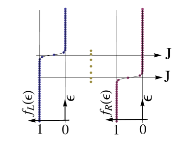
Figure 1: Schematic plot of the left and right Fermi distributions and the levels of the middle chain with $N=7$ sites.

In Fig. 1 we depict in blue and red two Fermi distributions with $K=50$ levels and parameters $\mu_{L}=4,\beta_{L}=3$ and $\mu_{R}=-4,\beta_{R}=3$ respectively. In the middle (brown) the spectrum of a chain with $7$ sites and $t=3.$ The width of the chain energy band is $4t$ with $7$ levels inside and is centered around $U=0$. From this picture, we expect that decreasing the width $\Delta\mu$ of the populated energy interval $[\mu_{R},\mu_{L}]$ is equivalent to increase the width of the conduction band $t$. This is confirmed in the left panel of Fig. 2 where we show that the current is roughly independent of $t$ for $2t<\mu_{L}$ and decreases with $t$ for $2t>\mu_{L}$ (black dots), when the conduction band extends beyond the region populated by electrons in the reservoirs. The red dots are obtained for a larger $\Delta\mu$ for which the conduction band is always inside the populated region. In the rest of our numerical examples we set $U=0$ and $t=1$. Analogously, in the right panel of Fig. 2 we show that for fixed $t$ the current grows linearly with $\Delta\mu$ and saturates at $\Delta\mu>4t$.

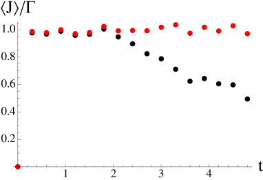
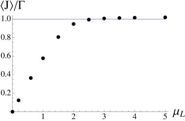
Figure 2: Current versus hopping $t$ for $\gamma=0.1,\,U=0$, $\beta_{L}=\beta_{R}=5$ , $v_{L}=v_{R}=0.05$, $K=200$ and $N=10$. In the left panel (black) $\mu_{L}=4,\ \mu_{R}=-4$ and (red) $\mu_{L}=10,\ \mu_{R}=-10$. Right panel: Same parameters except: $t=1,\,v_{L}=v_{R}=0.03$.

What is perhaps more interesting is the scaling of the current with $\Gamma=\Gamma_{L}\Gamma_{R}/(\Gamma_{L}+\Gamma_{R})$. In Fig. 3 we plot the current $\langle J\rangle$ as a function of the coupling to the right lead, showing that the main trend of the current is $\langle J\rangle=\Gamma$. In the inset we show that there are deviations to this law.

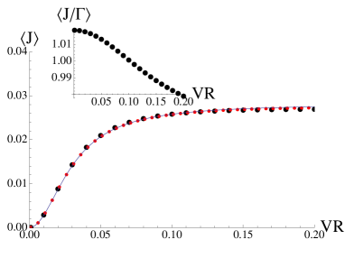
Figure 3: Black points are obtained by our model with $\gamma=0.1,\,\beta_{L}=\beta_{R}=5,\,\mu_{R}=-4,\,\mu_{L}=4;N=10,\,U=0,\,t=1,\,v_{L}=0.03,\,K=200$ and $E_{\rm min}=-20,\,E_{\rm max}=20$. The red dots are obtained by a numerical computation of the Landauer formula with $T=0$, and the continuous line is $\langle J\rangle=\Gamma=2\pi\frac{v_{R}^{2}v_{L}^{2}}{\theta_{0}(v_{L}^{2}+v_{R}^{2})}$. The inset is $\langle J\rangle/\Gamma$.

We have analyzed this behavior using the Landauer formula, that allows deeper analytical exploration. Since temperature is very low we take it exactly zero in both reservoirs, thus the Landauer formula is $\langle J\rangle=\Gamma_{L}\Gamma_{R}/2\pi\int_{\mu_{L}}^{\mu_{R}}{\rm tr}[G^{+}(\omega)G^{-}(\omega)].$ Changing the representation of the Green matrix from position basis to the energy basis (of the isolated chain) one can see that it is possible to approximate (isolated resonances approximation) the integrand as a superposition of $N$ Lorentzians each located at $2t\cos[j\pi/(N+1)]$ and with a width $(\Gamma_{L}+\Gamma_{R})\sin^{2}[j\pi/(N+1)]/(N+1),\,j=1,\ldots N$ along the energy axis. If $t<\mu_{L}$, the integral can be extended from $-\infty$ to $\infty$ because the Green function decays exponentially outside the energy band of the chain, thus the result $\langle J\rangle=\Gamma$ is obtained.

Now we can also explore fluctuations and compute $\langle J^{2}\rangle$. In Fig.4a, we computed for the same parameters than in Fig.2a the quantity $2\langle J^{2}\rangle/t^{2}-1$. We see that as soon as the current decreases because some modes of the chain goes out of the populated energy region, the fluctuation increases. As a function of other parameters like $v_{\alpha}$ or $N$ (data not shown), the average $\langle J^{2}\rangle$ does not have important changes (see Fig.4b).

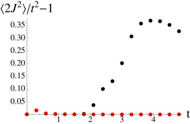
Figure 4: Panel a: $2\langle J^{2}\rangle/t^{2}-1$ as function of $t$ for $\mu_{R}=-4,\,\mu_{L}=4$ (black dots) and $\mu_{R}=-10,\,\mu_{L}=10$ (red dots) as in Fig. 2a. Panel b: $2\langle J^{2}\rangle/t^{2}-1$ for $t=3$ as a function of $v_{L}=v_{R}$. In both figures the other parameters are: $\gamma=0.1,\,\beta_{L}=\beta_{R}=5,N=10,\,U=0,\,K=200$ and $E_{\rm min}=-20,\,E_{\rm max}=20$ with $v_{L}=0.03$ in panel a and $t=3,\mu_{R}=-4,\mu_{L}=4$ in panel b.

IV conclusions

We showed that in the wide-band limit, the numerical results found in our model indeed correspond to what is expected on the basis of the Landauer formula, a formula which is usually interpreted as if the reservoirs were always in an equilibrium (gran canonical) distribution, not perturbed by the presence of the system. The Landauer formula emphasizes the role of the Fermi distributions of the reservoirs and provides an accurate description of the current if the assumption of reflectionless contacts is justified. In this respect, a very interesting relation was found in Shigeru and proved in mariborg between the current and the occupation of the meso-reservoir $\langle J\rangle=\sum_{k=1}^{K}2\gamma_{k}[\langle n^{L}_{k}\rangle-F_{L}(\varepsilon_{k})]$. This is an exact relation that in the appropriate limit should converge to the Landauer formula. Note that it implies that the occupation difference with respect to the Fermi distribution is ${\mathcal{O}}(\Gamma/\theta_{0}\gamma)$. It is a very interesting relation because it links the current, which is the fingerprint of the non equilibrium state, to the difference in distribution to the equilibrium case. Something similar has been found in classical systems where the fractal nature of the non equilibrium state is determined by the current gaspard . Moreover in  Shigeru we analyzed how Onsager reciprocity relation is broken in the system and found that $|L_{up}/L_{pu}-1|$ grows with $\gamma$ implying that despite the almost $\gamma$ independent value of the current, the dissipative mechanisms in the super-reservoir play an important role. A deeper study of these effects, that are beyond the Landauer picture, can be studied in the context of the model presented here and deserve further investigation.

References

• (1) W Aschbacher, V Jaǩsić, Y Pautrat, and C Pillet, J. Math. Phys. 48, 032101 (2007).
• (2) S. Ajisaka, F. Barra, C.Mejia-Monasterio and T. Prosen arXiv:1204.1321
• (3) S. Ajisaka, F. Barra, C.Mejia-Monasterio and T. Prosen, arXiv:1205.1167.
• (4) D. Ruelle J. Stat. Phys. 98, 57 (2000); Comm. Math. Phys. 224, 3 (2001).
• (5) S. Ajisaka, S. Tasaki and F. Barra, Bussei-Kenkyu 97 483 (2011/2012); arXiv:1110.6433
• (6) H. Wichterich, M. Henrich, H-P. Breuer, J. Gemmer, and M. Michel, Phys. Rev. E 76, 31115 (2007).
• (7) T. Prosen, N. J. Phys. 10, 3026 (2008).
• (8) A. A. Dzhioev and D. S. Kosov, J. Chem. Phys. 044121 134 (2011).
• (9) T. Prosen J. Stat. Mech. P077020 (2010).
• (10) S. Datta, Electronic Transport in Mesoscopic Systems (Cambridge University Press, Cambridge, 1995).
• (11) M. Zilly, Electronic conduction in linear quantum systems: Coherent transport and the effects of decoherence PhD. dissertation Universität Duisburg-Essen (http://duepublico.uni-duisburg-essen.de/servlets/DerivateServlet/Derivate-24279/dissertation_zilly.pdf).
• (12) F. Barra and P. Gaspard, J. Phys. A Math and Gen. 32 3357 (1999).
• (13) P. Gaspard, Chaos, Scattering and Statistical Mechanics (Cambridge University Press, Cambridge, 1998).