On the confinement of semiflexible chains under torsion

The following article has been accepted by JCP. After it is published, it will be found at J. Chem. Phys..

1 Introduction

The mechanical properties of biopolymers like DNA and actin are well described by a model of semiflexible polymers, characterized by a tangent-tangent correlation length that is considerably larger than the monomer size. A proper mathematical description is the worm-like chain (WLC): an elastic space curve with bending modulus $A$, that directly relates to this correlation length or orientational persistence length $P_{b}=A/k_{B}T$.

In the living cell biopolymers are usually in a crowded, strongly confined environment. Understanding the essential difference in statistics between the two extremes of the mechanical, strongly confined limit and the critical point of the self avoiding random walk limit, was an important development in polymer physics. In the first limit, the so called Odijk regime, the confining potential dominates on length scales shorter than the persistence length while in the latter case, the deGennes regime, the excluded volume interaction dominates the thermal fluctuations on length scales of the channel diameter. The general picture is the following [16]. Starting from strong confinement in a narrow channel: the polymer has due to its stiffness no other option than to follow the channel monotonously. The length scale over which the polymer is unperturbed by the confining potential, the so called deflection or collision length, is the dominating length scale. Upon increasing the channel size, or decreasing the potential strength, hairpins will form inverting the direction of the backbone of the polymer. The average distance between hairpins, the so called global persistence length, decreases with increasing channel size and becomes the length scale that determines the span of the polymer until this global persistence length becomes of the order of the orientational persistence length. At that point the a transition regime sets in in which the volume interactions, needed in the traditional de Gennes regime, are non existent relative to the thermal energy. This is a consequence of the slender shape of the polymer. Finally for channel sizes considerably larger than the orientational persistence length, when the channel-length over which the volume interactions have to be added to account for at least $1\>k_{B}T$ shrinks to the diameter of the channel, the de Gennes description becomes applicable.

The reduction in degrees of freedom caused by the confinement, can be expressed as an entropic cost that is often a decisive ingredient to statistical physics calculations, for systems in thermal equilibrium, but also for the dynamics of the system. Examples are the nematic transition of semiflexible polymers, the ejection of DNA from viral capsids [12], translocation of DNA through nanopores [14], the elongation and dynamics of DNA in nanochannels [19] and the dynamics of actin networks [6]. From an application point of view the possibility to lay out DNA almost fully stretched in a nanochannel makes it possible to study DNA and its interaction with proteins on the base pair level [18].

In many cases the WLC model is not sufficient though and it becomes crucial to understand how twist effects change this picture. This is for example the case in understanding the physics of transcription, the dynamics of supercoiling of DNA in vivo and the torque molecular motors can produce. In this paper the influence of torque on the confinement of a semiflexible chain is studied in the Odijk regime. It will be shown how as a consequence fluctuations in the confined directions get coupled. Also the influence of torque on the global persistence length is studied. An important result is a dramatic decrease of the elongation of DNA in nanochannels under moderate torques.

The paper is organized as follows: In section 2 we set up the model and its Hamiltonian. We first consider an isotropic channel and show how the parametrization can be changed from a potential strength to a deflection length. We next proceed to treat the general anisotropic case. In section 3 we discuss some refinements, like the addition of a stretch- and twist-stretch–moduli, how to map the model to hard-walled channels and we briefly discuss how torque influences the elongation problem in nanochannels.

2 The model

The free energy of a freely rotating semiflexible chain in a confining harmonic potential was calculated in Ref. [2]. These calculations we now perform for a persistent chain under torsion. In fact confinement by a constant harmonic potential is usually not what is needed. In case of a hard-walled nanochannel, the width of the channel is better approximated by a fixed standard deviation than a harmonic potential. The confining potentials in vivo and in single molecule experiments are usually also far from harmonic, while the standard deviation of the channel is used as a variational parameter [20, 3]. Nonetheless the harmonic potential is used as a Lagrange multiplier, an artificial confining potential to set the standard deviation $\sigma$ of the transversal polymer distribution as measure of width of the confinement. The benefit is an analytically solvable model and as long as the confinement is strong enough specification of the second moment of the chain distribution will do.

The typical length scale, that determines the physical properties is the deflection-length $\lambda=\sqrt[3]{P_{b}\sigma^{2}}$ of the chain, the length above which confinement dominates thermal fluctuations. The main calculations will be performed in a fixed number of turns, or linking number $\operatorname{Lk}$, ensemble. To keep the treatment transparent we model the persistent chain as a framed space-curve with a persistence-length $P_{b}$ and a torsional persistence length $P_{c}$. The results are easily extended with a finite stretch modulus $S$ and a twist-stretch coupling, $B$ [13]. All energies are scaled by $k_{B}T$ (unless mentioned) for notational reasons. As a result forces have the dimension of an inverse length.

The chain is confined in two perpendicular directions, say $x$ and $y$, by a harmonic potential. As in Ref. [2], we assume the confinement to be strong enough for the $z$-coordinate to be a single valued function of the curve. The framing is needed to describe the twist degree of freedom. Since the confinement potential is localized in space we cannot resort to the usual tangential description but have to start from the space curve [2]. The Hamiltonian is:

$$\begin{split}\mathscr{H}={}&\int_{0}^{L_{c}}\!\mathrm{d}s\left[\frac{P_{b}}{2}\left(\frac{\mathrm{d}^{2}\mathbf{r}(s)}{\mathrm{d}s^{2}}\right)^{2}\!+\frac{P_{c}}{2}\dot{\psi}^{2}(s)\right.\\ &+\left.\frac{b_{x}}{2}r_{x}^{2}(s)+\frac{b_{y}}{2}r_{y}^{2}(s)\right].\end{split}$$ (1)

As parametrization we choose the arc-length of the chain. The strength of the harmonic potential is set by $b_{x,y}$. The twist angle $\psi(s)$ is defined as follows: let $\mathbf{t}(s)=\dot{\mathbf{r}}(s)$ be the tangent and $\mathbf{n}(s)$ be one of the unit normals that define the local frame. The twist density is defined as the differential number of rotations of $\mathbf{n}$ around the tangential direction: $\operatorname{tw}(s)=\frac{1}{2\pi}(\mathbf{t}\wedge\mathbf{n})\cdot\mathbf{\dot{n}}$, which is a total differential and so we can define $\dot{\psi}(s):=2\pi\operatorname{tw}(s)$,

The twist density is not a small parameter and it is not independent of the radial fluctuations. To perform a perturbation expansion we split of the independent fluctuation degrees of freedom. This we can do using White’s relation [21, 4], relating linking number, twist $\operatorname{T\!w}$, and writhe $\operatorname{W\!r}$ (the Gauss linking number of a closed curve with itself):

$$\operatorname{T\!w} :=\int_{0}^{L_{c}}\mathrm{d}s\operatorname{tw}=\operatorname{Lk}-\operatorname{W\!r}$$ (2)

By assumption the chain is almost fully elongated permitting us to take periodic boundary conditions. With this choice are the tangents at the ends of the chain parallel. Since $2\pi$ times the writhe+1 of a closed curve is equal to the surface on the direction sphere enclosed by the path of the tangent mod $4\pi$ [5], and the tangents at both ends are parallel, we can define the writhe of the chain as the area enclosed by the tangent along the contour, implicitly setting the $0$ of the writhe to be the $z$-axis. Since the $z$-coordinate is single valued we can use Fuller’s equation [5, 1] turning the writhe of the chain in an integral over a writhe density $\omega$ that is up to quadratic order in the fluctuations:

$$\operatorname{wr}(s) \simeq\frac{1}{4\pi}(\dot{r}_{x}(s)\ddot{r}_{y}(s)-\ddot{r}_{x}(s)\dot{r}_{y}(s))$$ (3)

The linking number density we define as $lk:=\operatorname{Lk}/L_{c}$. Now define a fluctuation field $\phi(s):=\dot{\psi}-2\pi lk-2\pi\operatorname{wr}(s)$. From Eq. (2) it follows that $\int_{0}^{L_{c}}\mathrm{d}s\phi(s)=0$. We use this to eliminate the twist term and can now integrate out the independent field $\phi$. Making use of Eq. (3) results up to second order and an irrelevant constant in:

$$\begin{split}\mathscr{H}={}&\int_{0}^{L_{c}}\mathrm{d}s\left[\frac{P_{b}}{2}\mathbf{\ddot{r}}^{2}\!+\frac{b_{x}}{2}r_{x}^{2}+\frac{b_{y}}{2}r_{y}^{2}\right.\\ &-\left.\pi P_{c}lk(\dot{r}_{x}\ddot{r}_{y}-\ddot{r}_{x}\dot{r}_{y})\right]+2\pi^{2}P_{c}lk^{2}L_{c}\end{split}$$ (4)

The first term contains up to quadratic order only the $x$ and $y$ components since the $z$ component of the tangent vector $\mathbf{t}(s)$ is quadratic in the fluctuations:

$$\mathbf{\ddot{r}}^{2}(s)=\dot{t}_{x}(s)^{2}+\dot{t}_{y}(s)^{2}+\dot{t}_{z}(s)^{2}\simeq\dot{t}_{x}(s)^{2}+\dot{t}_{y}(s)^{2}$$ (5)

In the following we will take $\mathbf{r}$ to be two-dimensional. For reasons of clarity we present the analysis in more detail for an isotropic confinement

2.1 Isotropic confinement

For isotropic confinement we have $b:=b_{x}=b_{y}$. We can get rid of some of the coupling constants by appropriately scaling the contour lengths and the channel width [2]

$$\hat{s} =b^{1/4}P_{b}^{-1/4}s \breve{r_{i}} =P_{b}^{1/8}b^{3/8}\mathbf{r_{i}}$$ (6)

and so $\hat{P_{c}}=b^{1/4}P_{b}^{-1/4}P_{c}$ but $\hat{lk}=b^{-1/4}P_{b}^{1/4}lk$. This scaling results in:

$$\begin{split}\mathscr{H}={}&\int_{0}^{\hat{L_{c}}}\mathrm{d}\hat{s}\left[\frac{1}{2}\ddot{\breve{\mathbf{r}}}^{2}(\hat{s})+\frac{1}{2}\breve{\mathbf{r}}^{2}(\hat{s})-\frac{1}{2}\zeta(\dot{\breve{r}}_{x}\ddot{\breve{r}}_{y}-\ddot{\breve{r}}_{x}\dot{\breve{r}}_{y})\right]\\ &+2\pi^{2}\hat{P_{c}}\hat{lk}^{2}\hat{L_{c}}\end{split}$$ (7)

with

$$\zeta=\frac{2\pi P_{c}lk}{P_{b}^{3/4}b^{1/4}}$$ (8)

The configurational partition sum is a path integral over the two-dimensional field $\breve{\mathbf{r}}$:

$$Z=\int\mathcal{D}(\breve{\mathbf{r}})e^{-\mathscr{H}}$$ (9)

The last term of the Hamiltonian is constant and can be taken out from under the path integral. It represents the unperturbed twist energy. What is left is the fluctuation part which can be diagonalized, after a Fourier mode expansion using periodic boundary conditions, with eigenvalues:

$$ev_{n,\pm} =p_{n}^{4}+1\pm\zeta p_{n}^{3} \text{with }p_{n} =\frac{2\pi n}{\hat{L_{c}}}$$ (10)

Negative eigenvalues appear when $\zeta\geq\zeta_{cr}=4/3^{3/4}$ and so one can speak of a critical linking number density: $lk_{cr}=2b^{1/4}P_{b}^{3/4}/(3^{3/4}\pi P_{c})$. The partition sum $Z=\int[\mathcal{D}\mathbf{r}]\exp[-\mathscr{H}]$, becomes a product of Gaussian integrals, that can be compared to the free chain [11]. The result can be written as:

$$Z =\mathcal{N}\exp(-2\pi^{2}\hat{P_{c}}\hat{lk}^{2}\hat{L_{c}})\prod_{n=1}^{\infty}\frac{p_{n}^{8}}{ev_{n,+}ev_{n.-}}$$ (11)

with $\mathcal{N}$ collecting constant terms. In the denominator of the product we have a quartic expression in $n^{2}$: Let $\eta_{i},\bar{\eta}_{i}(i=1,2)$ be the pairs of conjugate roots:

$$(\eta_{i}^{2}+1)^{2}-\zeta^{2}\eta_{i}^{3}=0.$$ (12)

Then we can write the product as:

$$\prod_{n=1}^{\infty}(\cdots) =\prod_{i=1,2}\prod_{n=1}^{\infty}\frac{1}{\left(1-\frac{\eta_{i}}{n^{2}}\right)}\frac{1}{\left(1-\frac{\bar{\eta}_{i}}{n^{2}}\right)}$$

$$=\prod_{i=1,2}\frac{\pi\sqrt{\eta_{i}}}{\sin(\pi\sqrt{\eta_{i}})}\frac{\pi\sqrt{\bar{\eta}_{i}}}{\sin(\pi\sqrt{\bar{\eta}_{i}})}$$ (13)

The complex part of the square root of the $\eta_{i}$’s give an exponential decay with increasing chain length. Now write $\sqrt{\eta_{1,2}}=\frac{\hat{L}}{2\pi}(x_{1,2}\pm\imath y_{1,2})$. In the long chain limit, as long as the $y_{i}$ are non-zero we obtain the free energy density as:

$$\mathfrak{f}=\lim_{L_{c}\to\infty}-\frac{1}{L_{c}}\log Z =2\pi^{2}P_{c}lk^{2}+\frac{\bigl{(}P_{b}^{3}b\bigr{)}^{1/4}}{P_{b}}(|y_{1}|+|y_{2}|)$$ (14)

Figure 1: Flow of the roots $\sqrt{\eta_{i}}$ in the complex plane under increasing torsion. The size of the arrows indicates the speed with which the roots flow as explained in the text.

The first term is the zero-temperature twist energy density stored in the chain, the second $\mathfrak{f}_{th}$ the thermal fluctuation contribution in presence of the confining potential. In case the linking number density is zero, the roots are up to a sign equal: $|y_{1,2}|=1/\sqrt{2}$ and we retrieve Burkhardt’s result [2]. The flow of the roots under increasing linking number density is depicted in Fig. 1. Starting from $lk=0$ the root pairs move apart. Both decrease their imaginary parts, decreasing the free energy. This does not happen in a symmetric way, as is shown by the line segments along trajectories, where each segment corresponds to a fixed increase of $lk$, the arrow pointing in the direction of the flow. At $lk_{cr}$ the right pair of roots becomes real indicating a singularity in the partition sum.

As explained above the harmonic potential is only there to set the confinement. The target is to express all quantities in the standard deviations of the transversal distributions of the chain in the channel. To do this and to extend the calculations to a non-isotropic confinement we perform the previous calculations in an alternative way, taking first the logarithm of Eq. (11) and then the infinite chain limit:

$$\mathfrak{f}_{th}={} -\frac{1}{L_{c}}\log Z$$

$$={} -\frac{1}{L_{c}}\sum_{n=1}^{\infty}\log\left(\frac{p_{n}^{8}}{(p_{n}^{4}+1)^{2}-\zeta^{2}p_{n}^{6}}\right)+\mathcal{O}\big{(}\tfrac{\log(L_{c})}{L_{c}}\big{)}$$

$$\simeq{} -\frac{\bigl{(}P_{b}^{3}b\bigr{)}^{1/4}}{P_{b}}\int_{0}^{\infty}\frac{\mathrm{d}p}{2\pi}\log\left(\frac{p^{8}}{(p^{4}+1)^{2}-\zeta^{2}p^{6}}\right)$$

$$={} -\frac{2\pi P_{c}lk}{P_{b}\zeta}\left[-\sqrt{2}-\int_{0}^{\infty}\frac{\mathrm{d}p}{2\pi}\log\left(1-\frac{\zeta^{2}p^{6}}{(p^{4}+1)^{2}}\right)\right]$$ (15)

expanding the logarithm, making use of the fact that $\zeta p^{3}<p^{4}+1$, for $\zeta<\zeta_{cr}$, and noting that the series converges uniformly in any closed interval contained in $[0,\zeta_{cr})$ this results in:

$$\mathfrak{f}_{th}={} -\frac{2\pi P_{c}lk}{P_{b}\zeta}\left[-\sqrt{2}+\sum_{n=1}^{\infty}\frac{1}{n}\int_{0}^{\infty}\frac{\mathrm{d}p}{2\pi}\left(\frac{\zeta^{2}p^{6}}{(p^{4}+1)^{2}}\right)^{n}\right]$$

$$={} \frac{2\pi P_{c}lk}{P_{b}\zeta}\sum_{n=0}^{\infty}a_{n}\zeta^{2n}\qquad\text{with: }a_{n}:=-\frac{\Gamma(\frac{n}{2}-\frac{1}{4})\Gamma(\frac{3n}{2}+\frac{1}{4})}{4\pi(2n)!}$$ (16)

This can be written as a linear combination of generalized hypergeometric functions:

$$\mathfrak{f}_{th}={} -\frac{2\pi P_{c}lk}{P_{b}\zeta}\sqrt{2}\left[1-\mbox{$\,{}_{3}${F}${}_{2}\!$}\left(-\tfrac{1}{4},\tfrac{1}{12},\tfrac{5}{12};\tfrac{1}{4},\tfrac{1}{2};\tfrac{\zeta^{4}}{\zeta_{cr}^{4}}\right)\right.$$

$$\left.\qquad+\frac{3\zeta^{2}}{32}\mbox{$\,{}_{3}${F}${}_{2}\!$}\left(\tfrac{1}{4},\tfrac{7}{12},\tfrac{11}{12};\tfrac{3}{4},\tfrac{3}{2};\tfrac{\zeta^{4}}{\zeta_{cr}^{4}}\right)\right],$$

making the bifurcation point $\zeta_{cr}$ explicit. Defining:

$$x :=\frac{\zeta}{\zeta_{cr}} \gamma :=\sqrt{2}\frac{2\pi P_{c}lk}{P_{b}\zeta_{cr}},$$ (17)

results in a free energy density given by:

$$\frac{\mathfrak{f}_{th}}{\gamma} =\sum_{n=0}^{\infty}a_{n}x^{2n-1}=\frac{1}{x}-\frac{x}{2\sqrt{3}}-\frac{5x^{3}}{72}+\mathcal{O}(x^{7})$$ (18)

From the series expansion of $\mathfrak{f}_{th}$ it is straightforward to find a series expansion for the standard deviation $\sigma_{r}=\sqrt{\left\langle\mathbf{r}^{2}\right\rangle/2}$ of the transversal position of the chain in the channel:

$$\sigma_{r}^{2}=\frac{\partial\mathfrak{f}_{th}}{\partial b}=-\frac{1}{P_{b}\gamma^{3}}\sum_{n=0}^{\infty}(2n-1)a_{n}x^{2n+3},$$ (19)

which is again a linear combination of generalized hypergeometric functions. We now apply Lagrange inversion to this series in order to eliminate $b$ in favor of $\sigma_{r}$ as dependent parameter for the free energy density. To be able to use Lagrange inversion the derivative at the point of inversion should be non-zero, which requires non-zero coefficients of the linear term. The lowest term in Eq. (19) is cubic, so if we take the cubic root of this series we obtain a series to which one can apply Lagrange inversion. Introducing the deflection length, $\lambda:=(P_{b}\sigma_{r}^{2})^{1/3}$ we start from its series expansion:

$$\begin{split}\lambda(x)={}&\frac{\sqrt[3]{a_{0}}}{\gamma}x\\ &+\frac{\sqrt[3]{a_{0}}}{\gamma}x\sum_{k=1}^{\infty}\frac{\Gamma(-\tfrac{1}{3}+k)}{k!\Gamma(-\tfrac{1}{3})}\left(\sum_{n=1}^{\infty}(2n-1)\frac{a_{n}}{a_{0}}x^{2n}\right)^{k},\end{split}$$ (20)

and apply Lagrange inversion to this:

$$x(\lambda) =\sum_{n=1}^{\infty}\frac{1}{n!}\left.\frac{\mathrm{d}^{n-1}}{\mathrm{d}x^{n-1}}\left(\frac{x}{\lambda(x)}\right)^{n}\right\rvert_{x=0}\lambda^{n}$$ (21)

The first terms of the resulting series are:

$$x(\lambda) =\gamma\lambda-\frac{\gamma^{3}\lambda^{3}}{6\sqrt{3}}-\frac{7\gamma^{5}\lambda^{5}}{216}+\mathcal{O}\left((\gamma\lambda)^{7}\right)$$

$$\mathfrak{f}_{th}(\lambda) =\frac{1}{\lambda}-\frac{\gamma^{2}\lambda}{3\sqrt{3}}+\frac{5\gamma^{6}\lambda^{5}}{243\sqrt{3}}+\mathcal{O}({z^{7/3}})$$

or in terms of the unscaled variables:

$$\begin{split}\mathfrak{f}_{th}={}&\frac{1}{\lambda}\left[1-\frac{1}{2}\left(\pi P_{c}lk\frac{\lambda}{P_{b}}\right)^{2}\right.\\ &\left.+\frac{5}{24}\left(\pi P_{c}lk\frac{\lambda}{P_{b}}\right)^{6}+\mathcal{O}\Bigl{(}\left(\pi P_{c}lk\frac{\lambda}{P_{b}}\right)^{8}\Bigr{)}\right]\end{split}$$ (22)

This free energy density contains the enthalpic free energy of the harmonic potential. But the harmonic potential is just a Lagrange multiplier to set the standard deviation, thus this enthalpic part of the confining potential should be subtracted in order to obtain the net cost for confining the molecule. The enthalpic contribution is easily calculated from the inverted series:

$$\mathfrak{f}_{pot}={} \frac{1}{2}b\left\langle\mathbf{r}^{2}\right\rangle=\frac{27}{16}\left(\frac{\pi P_{c}lk}{P_{b}}\right)^{4}\frac{\lambda^{3}}{x^{4}(\lambda)}$$

$$\begin{split}={}&\frac{1}{\lambda}\left[\frac{1}{4}+\frac{1}{4}\left(\pi P_{c}lk\frac{\lambda}{P_{b}}\right)^{2}+\frac{3}{8}\left(\pi P_{c}lk\frac{\lambda}{P_{b}}\right)^{4}\right.\\ &\qquad\left.+\mathcal{O}\Bigl{(}\left(\pi P_{c}lk\frac{\lambda}{P_{b}}\right)^{6}\Bigr{)}\right]\end{split}$$ (23)

Subtracting this free energy density from Eq. (22) gives the confinement free energy density:

$$\begin{split}\mathfrak{f}_{conf}={}&\frac{1}{\lambda}\left[\frac{3}{4}-\frac{3}{4}\left(\pi P_{c}lk\frac{\lambda}{P_{b}}\right)^{2}-\frac{3}{8}\left(\pi P_{c}lk\frac{\lambda}{P_{b}}\right)^{4}\right.\\ &\qquad\left.+\mathcal{O}\Bigl{(}\left(\pi P_{c}lk\frac{\lambda}{P_{b}}\right)^{6}\Bigr{)}\right]\end{split}$$ (24)

Note that the free energy of confinement seems to decrease with increasing linking number, while the standard deviation is kept constant. This is actually the twist energy reduction due to thermal writhe. The unperturbed twist energy density was the last term in Eq. 7 adding the perturbation contribution we recover the effective twist free energy density:

$$\mathfrak{f}_{twist} =2\pi^{2}P_{c}\left(1-3\frac{P_{c}\lambda}{8P_{b}^{2}}\right)lk^{2}:=2\pi^{2}\bar{P}_{c}lk^{2},$$ (25)

where a “renormalized” torsional persistence length $\bar{P}_{c}$, is defined that is of the same form as that of a WLC under tension [15]. From Eq. (4) we see that the linking number density is conjugate to the thermal writhe density in $\mathfrak{f}_{th}$, allowing us to calculate its expectation value and from White’s equation the expectation value of the twist density:

$$\left\langle\operatorname{wr}\right\rangle \simeq-\frac{1}{4\pi^{2}P_{c}}\frac{\partial\mathfrak{f}_{th}(lk,b)}{\partial lk}=\frac{3P_{c}\lambda lk}{8P_{b}^{2}}$$ (26)

$$\left\langle\operatorname{tw}\right\rangle \simeq lk-\left\langle\operatorname{wr}\right\rangle=\left(1-\frac{3P_{c}\lambda}{8P_{b}^{2}}\right)lk$$ (27)

Thermal motion decreases the extension of the chain. It is calculated by adding a tension term in the channel direction to the Hamiltonian:

$$\mathscr{H}\rightarrow\mathscr{H}+Fz \simeq\mathscr{H}+\int_{0}^{L_{c}}\mathrm{d}sF(1-\frac{1}{2}\dot{\mathbf{r}}^{2}(s)).$$ (28)

The extension in the $z$-direction is $\rho:=\Delta z/L_{c}=\partial_{F}\mathfrak{f}(F)|_{F=0}$. After a mode expansion the fluctuation part can be diagonalized again with $F$ dependent eigenvalues. The calculation of the free energy density goes as before:

$$\mathfrak{f}_{th}=-\frac{\bigl{(}P_{b}^{3}b\bigr{)}^{1/4}}{P_{b}}\left[\int_{0}^{\infty}\frac{\mathrm{d}p}{2\pi}\log\left(\frac{p^{8}}{(p^{4}+\tfrac{F}{\sqrt{P_{b}b}}p^{2}+1)^{2}}\right)^{\mbox{}}\right.\\ \left.+\sum_{n=1}^{\infty}\frac{1}{n}\int_{0}^{\infty}\frac{\mathrm{d}p}{2\pi}\left(\frac{\zeta^{2}p^{6}}{(p^{4}+\tfrac{F}{\sqrt{P_{b}b}}p^{2}+1)^{2}}\right)^{n}\right]$$ (29)

For the contraction factor we obtain in terms of the deflection length:

$$\rho=1-\frac{\lambda}{2P_{b}}\left[1+\left(\pi P_{c}lk\frac{\lambda}{P_{b}}\right)^{2}+\mathcal{O}\Bigl{(}\left(\pi P_{c}lk\frac{\lambda}{P_{b}}\right)^{4}\Bigr{)}\right]$$ (30)

A last quantity that is easily extracted is the expectation value of the torque $\tau$ one has to apply to keep the linking number fixed:

$$\left\langle\tau\right\rangle=\frac{1}{2\pi}\frac{\partial\mathfrak{f}_{twist}}{\partial lk}=2\pi\bar{P}_{c}lk$$ (31)

The influence of torque on the confined polymer is small for a strong confinement. The restricted space around the polymer hinders the production of thermal writhe. Upon increasing the standard deviation thermal withe becomes stronger. In the torsionless case, the demand that the z-coordinate is a single valued function along the backbone results in the demand that the deflection length is much smaller than the persistence length. With torsion, this upper bound decreases with increasing torque. From the series (29), (30) it can be seen that the demand on deflection length changes to

$$\lambda\ll\frac{P_{b}}{\pi P_{c}lk}.$$ (32)

Using Eq. (31) this can be written as a torque dependent constraint on the standard deviation:

$$\sigma\ll P_{b}\left(\frac{8P_{b}}{3P_{c}+4P_{b}\tau}\right)^{3/2}$$ (33)

Note that $\tau$ is scaled by $k_{B}T$. In section 3 the effect of this approaching instability on the extension is discussed.

Figure 2: The local relative extension for DNA in a confined environment, producing a standard deviation up to $8$ nm with a range of torques applied along the backbone. The persistence lengths were chosen to be $P_{b}=50$nm and $P_{c}=100$nm

In Figure 2 the effect of a finite torque is shown on the semi-local extension of DNA, with torques that are realistic for torque producing molecular motors in vivo. It is important to realize that the strength of the harmonic potential needed to obtain a fixed standard deviation increases with increasing torque.

2.2 Non-isotropic confinement

The strategy for the non-isotropic case will be the same as for the isotropic case. The increased complexity is a consequence of the twist mixing fluctuations in the two transversal directions. The Hamiltonian is again block diagonalized after a Fourier expansion. With

$$b :=\frac{33(b_{x}^{2}b_{y}+b_{x}b_{y}^{2})+(b_{x}^{2}+14b_{x}b_{y}+b_{y}^{2})^{3/2}-b_{x}^{3}-b_{y}^{3}}{128b_{x}b_{y}}.$$ (34)

and a scaling like in the isotropic case we see that the expression for the critical point is, like in the isotropic case: $\zeta_{cr}=4/3^{3/4}$. We assume $\zeta$ to be small. Defining $\bar{b}_{x,y}:=b_{x,y}/b$ the fluctuation part of the free energy density can again be written as an integral over the determinants:

$$\mathfrak{f}_{th}=-\frac{\bigl{(}P_{b}^{3}b\bigr{)}^{1/4}}{P_{b}}\left[\int_{0}^{\infty}\frac{\mathrm{d}p}{2\pi}\log\left(\frac{p^{8}}{(p^{4}+\bar{b}_{x})(p^{4}+\bar{b}_{y})}\right)\right.\\ +\left.\sum_{n=1}^{\infty}\frac{\zeta^{2n}}{n}\int_{0}^{\infty}\frac{\mathrm{d}p}{2\pi}\left(\frac{p^{6}}{(p^{4}+\bar{b}_{x})(p^{4}+\bar{b}_{y})}\right)^{n}\right]$$ (35)

Assume $b_{x}\leq b_{y}$. Integration results in a power series in $\zeta$, with coefficients that can be expressed in series over hypergeometric functions. We will only need the first terms. They are:

$$\begin{split}\mathfrak{f}_{th}={}&\frac{\bigl{(}P_{b}^{3}b\bigr{)}^{1/4}}{P_{b}}\left(\frac{\bar{b}_{x}^{1/4}+\bar{b}_{y}^{1/4}}{\sqrt{2}}\right.\\ &\left.-\frac{\bar{b}_{x}^{1/2}+\bar{b}_{x}^{1/4}\bar{b}_{y}^{1/4}+\bar{b}_{y}^{1/2}}{4\sqrt{2}(\bar{b}_{x}^{1/4}+\bar{b}_{y}^{1/4})(\bar{b}_{x}^{1/2}+\bar{b}_{y}^{1/2})}\zeta^{2}+\mathcal{O}(\zeta^{4})\right).\end{split}$$ (36)

Since the terms in the series expansion are independent of the $b-$scale, we can choose it as $b=1/P_{b}^{3}$ and change from $b_{x,y}$ to the dimensionless $z_{x,y}:=\bigl{(}P_{b}^{3}b_{x,y}\bigr{)}^{-1/4}$ resulting in

$$\mathfrak{f}_{th} =\frac{1}{P_{b}}\left(\frac{z_{x}+z_{y}}{\sqrt{2}z_{x}z_{y}}-\frac{z_{x}z_{y}(z_{x}^{2}+z_{x}z_{y}+z_{y}^{2})}{4\sqrt{2}(z_{x}+z_{y})(z_{x}^{2}+z_{y}^{2})}\zeta_{1}^{2}+\cdots\right),$$ (37)

with $\zeta_{1}=2\pi P_{c}lk$. To get an expression for the free energy as function of the deflection lengths we will use a multivariate extension of Lagrange inversion [8, 7]. As in the isotropic case we extract the standard deviations for the two channel directions from the free energy density:

$$\sigma_{x}^{2} =-\frac{P_{b}^{3}}{2}z_{x}^{5}\partial_{z_{x}}\mathfrak{f}_{th}$$

$$=\frac{P_{b}^{2}z_{x}^{3}}{2\sqrt{2}}\left(1+\frac{z_{x}^{2}z_{y}^{4}(3z_{x}^{2}+2z_{x}z_{y}+z_{y}^{2})}{4(z_{x}+z_{y})^{2}(z_{x}^{2}+z_{y}^{2})^{2}}\zeta_{1}^{2}+\cdots\right),$$ (38)

and $z_{x}\leftrightarrow z_{y}$ for $\sigma_{y}$. With $f_{x,y}:=z_{x,y}/\lambda_{x,y}(zx,zy)$, we have a relation between $\lambda_{x,y}$ and $z_{x,y}$ of the right type to apply Good-Lagrange inversion, that is:

$$z_{x,y} =f_{x,y}\lambda_{x,y} \text{and }f_{x,y}(0,0)\neq 0.$$ (39)

Under these condition given any (formal) power series $g$ in $z_{x}$ and $z_{y}$ we can express $g$ uniquely as a power series in $\lambda_{x}$, $\lambda_{y}$ by the Good-Lagrange formula [8, 7]:

$$[\lambda_{x,y} ]^{n,m}g\bigl{(}z_{x}(u_{x}),z_{y}(u_{y})\bigr{)}$$

$$={} [z_{x,y}]^{n,m}g(z_{x},z_{y})f_{x}^{n}(z_{x},z_{y})f_{y}^{m}(z_{x},z_{y})$$

$$\qquad\operatorname{Det}\biggl{(}\delta_{i,j}-\frac{z_{i}}{f_{j}(z_{x},z_{y})}\frac{\partial f_{j}(z_{x},z_{y})}{\partial z_{i}}\biggr{)}$$

$$={} [z_{x,y}]^{n,m}g(z_{x},z_{y})f_{x}^{n}(z_{x},z_{y})f_{y}^{m}(z_{x},z_{y})$$

$$\qquad\frac{1}{9}\operatorname{Det}\biggl{(}\frac{z_{i}}{\sigma^{2}_{j}(z_{x},z_{y})}\frac{\partial\sigma^{2}_{j}(z_{x},z_{y})}{\partial z_{i}}\biggr{)},$$ (40)

where $[x_{1,2}]^{n,m}F(x_{1,2})$ denotes the coefficient of the monomial $x_{1}^{n}x_{2}^{m}$ in the (formal) power series $F$. When applied to $\mathfrak{f}_{th}$ we obtain a series that is symmetric against interchange of $\lambda_{x}$ and $\lambda_{y}$. We define the symmetrized monomial:

$$[n,m]:=\lambda_{x}^{n}\lambda_{y}^{m}+\lambda_{y}^{n}\lambda_{x}^{m}.$$ (41)

For $\mathfrak{f}_{th}$ we get:

$$\mathfrak{f}_{th}={} \frac{1}{2}[-1,0]-\frac{\zeta_{1}^{2}}{6P_{b}^{2}}([1,0]-[4,-3]$$

$$\quad+[5,-4]-[8,-7]+\cdots)+\mathcal{O}\Bigl{(}\zeta_{1}^{6}\Bigr{)}$$

$$\simeq{} \frac{1}{2}[-1,0]-\frac{\zeta_{1}^{2}}{6P_{b}^{2}}\frac{[3,1]+[2,2]/2}{[1,0][2,0]}$$

$$={} \frac{1}{2}(\lambda_{x}^{-1}+\lambda_{y}^{-1})-\frac{2(\pi P_{c}lk)^{2}}{3P_{b}^{2}}\frac{\lambda_{x}^{3}\lambda_{y}+\lambda_{x}^{2}\lambda_{y}^{2}+\lambda_{x}\lambda_{y}^{3}}{(\lambda_{x}+\lambda_{y})(\lambda_{x}^{2}+\lambda_{y}^{2})}$$ (42)

The combination of powers in the deflection lengths in the 2nd term will appear several times. For this reason we define an effective twist deflection length

$$\bar{\lambda} :=2\frac{\lambda_{x}^{3}\lambda_{y}+\lambda_{x}^{2}\lambda_{y}^{2}+\lambda_{x}\lambda_{y}^{3}}{(\lambda_{x}+\lambda_{y})(\lambda_{x}^{2}+\lambda_{y}^{2})}.$$ (43)

The factor $2$ is a matter of convention, chosen for comparison with the $P_{c}$ renormalization concept of a chain under tension of Ref. [15]. Let $\lambda_{x}$ be the smaller of the two deflection lengths, corresponding to the stronger confined direction, this effective deflection length has a value in between $\frac{3}{2}\lambda_{x}$ for $\lambda_{x}=\lambda_{y}$ and $2[1-(\lambda_{x}/P_{b})^{3}]\lambda_{x}$ for $\lambda_{x}<<\lambda_{y}$.

Apparently the thermal writhe effect on the free energy is dominated by the smallest deflection length. This is understandable since writhe is non-planar and since the polymer is directed along one axes, tightening one of the transversal directions forces the polymer to be more planar. Just like in the isotropic case we subtract the free energy contribution of the harmonic potential, to get the pure confinement free energy. The calculations are merely a repetition of the $\mathfrak{f}_{th}$ calculation so we just give the result up to the same order:

$$\mathfrak{f}_{pot} =\frac{1}{8}(\lambda_{x}^{-1}+\lambda_{y}^{-1})+\frac{(\pi P_{c}lk)^{2}}{6P_{b}^{2}}\bar{\lambda}$$

$$\mathfrak{f}_{conf} =\mathfrak{f}_{th}-\mathfrak{f}_{pot}=\frac{3}{8}(\lambda_{x}^{-1}+\lambda_{y}^{-1})-\frac{(\pi P_{c}lk)^{2}}{2P_{b}^{2}}\bar{\lambda}.$$ (44)

The second term can again be interpreted as a reduction of the twist free energy density. Adding it to the unperturbed twist free energy density we find:

$$\mathfrak{f}_{twist} =2\pi^{2}P_{c}\left(1-\frac{P_{c}\bar{\lambda}}{4P_{b}^{2}}\right)lk^{2}=:2\pi^{2}\bar{P}_{c}lk^{2},$$ (45)

the “renormalized” torsional persistence length $\bar{P}_{c}$, is again of the same form as the thermal softening of a WLC under tension [15]. The average writhe and twist densities follow from the same derivation as in the isotropic case, and using the Good-Lagrange formula for parameter change results in:

$$\left\langle\operatorname{wr}\right\rangle= \frac{\bar{\lambda}P_{c}lk}{4P_{b}^{2}} \left\langle\operatorname{tw}\right\rangle= \left(1-\frac{\bar{\lambda}P_{c}}{4P_{b}^{2}}\right)lk$$ (46)

The extension is calculated like before by adding a force term (28). We perform the derivation by $F$ before the integration, choose $b=P_{b}^{3}$ and expand in $\zeta_{1}$. The resulting extension is expressed in $z$

$$\rho =1-\frac{z_{x}+z_{y}}{4\sqrt{2}}-\frac{5}{16\sqrt{2}}\frac{z_{x}^{3}z_{y}^{3}}{(z_{x}+z_{y})(z_{x}^{2}+z_{y}^{2})}\zeta_{1}^{2}-\mathcal{O}(\zeta_{1}^{4})$$ (47)

Finally resorting again to Good-Lagrange inversion (2.2) we obtain

$$\begin{split}\rho={}&1-\frac{1}{4}\left(\frac{\lambda_{x}}{P_{b}}+\frac{\lambda_{y}}{P_{b}}\right)\\ &\quad-\frac{(7\lambda_{x}^{3}\lambda_{y}^{5}-2\lambda_{x}^{4}\lambda_{y}^{4}+7\lambda_{x}^{5}\lambda_{y}^{3})(\pi P_{c}lk)^{2}}{12(\lambda_{x}+\lambda_{y})(\lambda_{x}^{2}+\lambda_{y}^{2})^{2}P_{b}^{3}}.\end{split}$$ (48)

Also this last expression has the feature that it is the tightest direction that determines the thermal writhe.

Figure 3: The squeezing out of thermal writhe for DNA by anisotropy for $3$ different torques while keeping the influence of bending modes contant. The elastic moduli are chosen as in Fig. 2

In Figure 3 the extension of DNA upon non-isotropic confinement is shown. The amount of confinement anisotropy is changed by varying the standard deviations such that the sum of the two deflection lengths remains constant. In that way the contraction due to bending degrees of freedom does not change. The isotropic point is at $\sigma_{x}=\sigma_{y}=20$nm. In the limit of vanishing standard deviation in one direction, thermal writhe is completely suppressed.

3 Some extensions

We did not include a twist-stretch coupling, that is typically nonzero for chiral molecules, or or a stretch modulus in the calculations. To include them complicates the calculations only modestly. Mainly because the stretch modulus is large compared to tensions normally applied, their influence is small. In lowest order it amounts to a correction of the bare torsional persistence length to $P_{c}^{\prime}:=P_{c}-B^{2}/S$, where $B$ is the (dimensionless) twist-stretch coupling, and $S$ the stretch modulus [13]. Furthermore the contraction factor acquires a contribution: $\rho\rightarrow\rho-2\pi Blk/S$.

The calculations were performed using a harmonic potential as a substitute. To relate this to a hardwalled channel we can extend the reasoning from Ref. [20] and calculate the deflection length of the hard-walled channel, with channel width $d$, by comparing the confinement free energy at zero linking number density with the numerical results from Ref. [2, 22]. This leads to:

$$\lambda_{\mathrm{hard}}=\frac{3}{8\times 1.1036}(P_{b}d^{2})^{1/3}$$ (49)

One can reason now that since we have the free energy as function of the standard deviations, and thus up to this numerical factor of the channel dimensions, we can extend this to a finite torque. Had we used the potential strength b as parameter the chain would fluctuate through the channel wall.

A WLC under tension undergoes upon increasing linking number a buckling transition to a plectoneme, a critical multi-plectoneme phase or to a multitude of irregular configurations of loop-like structures (which might lead to structural changes in the WLC) [3]. Into which of these 3 categories the transition belongs depends on material and environmental parameters, but the linking number density is in all cases controlled by a mechanical instability at a critical linking number density of $lk_{cr}=\sqrt{FP_{b}}/(\pi P_{c})$. Comparing this with the instability in the confined chain, we see that the deflection lengths also here have a comparable role. The critical linking number density of the confined chain corresponds to that of a chain under tension $F$ when:

$$\sigma\cong\left(\frac{P_{b}}{F^{3}}\right)^{1/4}$$

As an important example we mention DNA where the maximum linking number density causing a buckling transition is for forces of around $4$ pN ($F=1\>\text{nm}^{-1}$), higher forces causing a structural transition within the DNA double helix. With a persistence length of $50$ nm this would correspond to a channel dimension $\sim 3\!$ nm, which is an order of magnitude smaller than the channels used in confinement experiments. In a plectoneme on the other hand the fluctuations of the strands can easily have comparable standard deviations [3], showing that plectonemes are indeed stable.

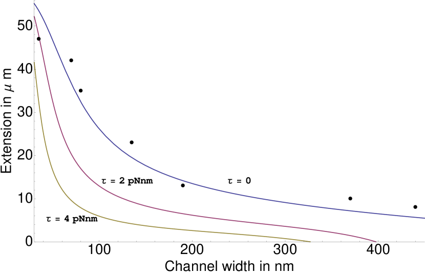
Figure 4: Extension of a 60 $\mu$m DNA chain in square nanochannels with widths from 30-450 nm, without torque and with torques of $2$ and $4$ pNnm ($\tau=0.5,1$), the dots are experimental data from Ref. [19]

With increasing channel size hairpin formation starts to influence chain extension [17] on top of local fluctuations. The free energy of an isolated hairpin in the mechanical limit, $\bar{F}_{mc}$ is in the torsionless case that of an entropically squeezed mechanical hairpin [17]. The hairpins seen as rare defects in the linear chain have a statistical density that increases exponentially with decreasing free energy of the hairpin. The global existence length is the average distance between hairpins When a torque is applied to a confined chain approaching the bifurcation point a local minimum will appear starting from an almost closed loop having a writhe close to one. In case the confinement is replaced by a tension, these loops form the nucleation point of plectonemes, super coiled helices perpendicular to the channel direction. The confinement does not allow for plectoneme formation and so the local minimum is the almost closed loop. These loops can not grow perpendicular to the channel axis, but can separate in two hairpins along the axes as shown in Fig. 5.

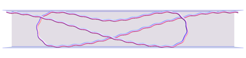
Figure 5: Two hairpins forming a planar loop of writhe $\simeq 1$

It can be shown [3] that when the tangent of the ground-state varies on a much larger length scale than the thermal fluctuations, the writhe of the ground-state and thermal writhe can be treated separately, the total writhe being their sum. Conceptually the thermal writhe can be calculated from Fuller’s equation with as reference curve the writhing ground-state. As long as this writhing ground-state is straight on the thermal fluctuations length scale the writhes separate. Since the confinement free energy (44) is only in higher order dependent on the linking number density, torque hardly influences the balance between entropic confinement and mechanical bending, that determines the hairpin free energy. The writhe of a pair of successive hairpins on the other hand does decrease the free energy and thereby the extension dramatically. In fact one can attribute a writhe of one half to a hairpin since two successive hairpins have this configuration as only minimum in their relative orientation, at least for a circular channel. Some minor contributions of other minima, reflecting the symmetry of the channel cross-section, might be present, but we will neglect them for the rest of the paper. Assuming the channel to be narrow enough that we can treat the hairpins as a dilute gas of defects we can follow the reasoning of Ref. [17]. The free energy of a hairpin in the mechanical limit decreases by the work done by the torque: $\bar{F}_{mc}(\tau)\simeq\bar{F}_{mc}(0)-\pi\tau$. Or in terms of the global persistence length:

$$g(\tau)=g(0)e^{-\pi\tau}$$ (50)

As example Figure 4 shows the effect of moderate $2$ pNnm ($\tau=0.5$) and $4$ pNnm ($\tau=1$) torques on the elongation of a $60$ $\mu$m DNA chain in a square channel with widths ranging from $40-100\quad\mu$m, following the theoretical treatment of Ref. [17] and in comparison with experiments from Reisner et al. [19] on DNA in nanochannels in the absence of torsion. The shortening by thermal fluctuations was calculated using equations (48),(31) and (49). As material parameters were used $P_{b}=57$ nm (DNA with dye as in Ref. [19]) and $P_{c}=100$ nm. Applying a moderate torque induces its collapse mainly due to the lowering of the hairpin free energy. Only above $350$ nm does the twist instability of confinement become important. A moderate torque of $2$ pNnm reduces the elongation to less than half the value it had in the torqueless case for channels larger than $90$ nm.

4 Summary and conclusion

As is shown in this paper, torsion can have a large impact on the confinement of semiflexible polymers. For nanosize confinement the thermal writhe caused by an applied torsion is damped by the tightest confinement direction. The apparent softening of the chain is similar to the softening of a semiflexible polymer under torsion [15] with the appearance of a new deflection length. The instability that appears in the free energy landscape sets new limits to the magnitude of the torque the molecule can propagate depending on the confinement of its environment. It is important that the strength of the confinement in one direction already suppresses the thermal writhe and thus increases the torque that propagates.

An important tool in the investigation of biopolymers and their interaction with proteins is the possibility to spread out the molecule in nanochannels of diameter [19, 10, 23, 18] comparable to the molecules persistence length. The theory presented here shows that torques that for example RNA-polymerase can induce [9] (up to $5$ pN nm) do increase the demands on channel size considerably.

References

- [1] J. Aldinger, I. Klapper, and M. Tabor. Formulae for the calculation and estimation of writhe. J. Knot Theor. Ramif., 4(3):343–372, 1995.
- [2] TW Burkhardt. Free energy of a semiflexible polymer confined along an axis. J. Phys. A: Math. Theor., 28:L629–L635, 1995.
- [3] M. Emanuel, G. Lanzani, and H. Schiessel. Multi-plectoneme phase of double-stranded dna under torsion. submitted, 2012.
- [4] F.B. Fuller. Writhing number of a space curve. PNAS, 68(4):815–&, 1971.
- [5] F.B. Fuller. Decomposition of the linking number of a closed ribbon: a problem from molecular biology. PNAS, 75(8):3557–3561, 1978.
- [6] ML Gardel, JH Shin, FC MacKintosh, L Mahadevan, P Matsudaira, and DA Weitz. Elastic Behavior of cross-linked and bundled actin networks. Science, 304(5675):1301–1305, 2004.
- [7] I.M. Gessel. A combinatorial proof of the multivariable Lagrange inversion formula. J. Comb. Theory, Ser. A, 45(2):178–195, 1987.
- [8] I.J. Good. Generalizations to several variables of Lagrange’s expansion, with applications to stochastic processes. Math. Proc. Camb. Philos. Soc., 56(4):367–380, 1960.
- [9] Y Harada, O Ohara, A Takatsuki, H Itoh, N Shimamoto, and K Kinosita. Direct observation of DNA rotation during transcription by Escherichia coli RNA polymerase. Nature, 409(6816):113–115, JAN 4 2001.
- [10] Kyubong Jo, Dalia M. Dhingra, Theo Odijk, Juan J. de Pablo, Michael D. Graham, Rod Runnheim, Dan Forrest, and David C. Schwartz. A single-molecule barcoding system using nanoslits for dna analysis. PNAS, 104(8):2673–2678, 2007.
- [11] Hagen Kleinert. Path Integrals in Quantum Mechanics, Statistics, Polymer Physics, and Financial Markets. World Scientific, 3rd edition, 2002.
- [12] Amelie Leforestier and Francoise Livolant. The Bacteriophage Genome Undergoes a Succession of Intracapsid Phase Transitions upon DNA Ejection. J. Mol. Biol., 396(2):384–395, FEB 19 2010.
- [13] J.F. Marko. DNA under high tension: overstretching, undertwisting, and relaxation dynamics. Phys. Rev. E, 57(2):2134–2149, 1998.
- [14] A Meller, L Nivon, E Brandin, J Golovchenko, and D Branton. Rapid nanopore discrimination between single polynucleotide molecules. PNAS, 97(3):1079–1084, FEB 1 2000.
- [15] J. David Moroz and Philip Nelson. Entropic elasticity of twist-storing polymers. Macromolecules, 31:6333–6347, 1998.
- [16] T. Odijk. Scaling theory of dna confined in nanochannels and nanoslits. Phys. Rev. E, 77(6):060901, 2008.
- [17] Theo Odijk. DNA confined in nanochannels: hairpin tightening by entropic depletion. J. Chem. Phys., 125(20):204904, 11 2006.
- [18] W. Reisner, J.N. Pedersen, and R.H. Austin. Dna confinement in nanochannels: physics and biological applications. Reports on Progress in Physics, 75(10):106601, 2012.
- [19] Walter Reisner, Keith J. Morton, Robert Riehn, Yan Mei Wang, Zhaoning Yu, Michael Rosen, James C. Sturm, Stephen Y. Chou, Erwin Frey, and Robert H. Austin. Statics and dynamics of single dna molecules confined in nanochannels. Phys. Rev. Lett., 94:196101, May 2005.
- [20] J. Ubbink and Theo Odijk. Electrostatic-undulatory theory of plectonemically supercoiled DNA. Biophys. J., 76(5):2502–2519, 1999.
- [21] James White. Self-linking and Gauss-integral in higher dimensions. Am. J. Math., 91(3):693–728, 1969.
- [22] Yingzi Yang, Theodore W. Burkhardt, and Gerhard Gompper. Free energy and extension of a semiflexible polymer in cylindrical confining geometries. Phys. Rev. E, 76:011804, Jul 2007.
- [23] Michael Zwolak and Massimiliano Di Ventra. Colloquium : Physical approaches to dna sequencing and detection. Rev. Mod. Phys., 80:141–165, Jan 2008.