Delay Equations of the Wheeler-Feynman Type

Abstract

We present an approximate model of Wheeler-Feynman electrodynamics for which uniqueness of solutions is proved. It is simple enough to be instructive but close enough to Wheeler-Feynman electrodynamics such that we can discuss its natural type of initial data, constants of motion and stable orbits with regard to Wheeler-Feynman electrodynamics.

Acknowledgements: The authors want to thank Gernot Bauer for enlightening discussions. D.-A.D. and N.V. gratefully acknowledge financial support from the BayEFG of the Freistaat Bayern and the Universität Bayern e.V.. This project was also funded by the post-doc program of the DAAD.

1 Introduction

Already in the early stages of classical electrodynamics it was observed that the coupled equations of motion of Maxwell and Lorentz for point-charges are ill-defined. Since then many attempts have been made to cure this problem among which the most famous one is Dirac’s mass renormalization [Dir38]. However, none of the known cures has yet led to a mathematically well-defined and physically sensible theory of relativistic interaction of point-charges. Rather than being a cure of the old theory, Wheeler-Feynman electrodynamics (WF) is a new formulation of classical electrodynamics and is maybe the most promising candidate for a divergence-free theory of electrodynamics about point-charges that is capable of describing the phenomenon of radiation damping [WF45, WF49]. For an overview on the mathematical and physical difficulties of classical electrodynamics and the role of WF we refer the interested reader also to the introductory sections of [BD01] and [BDD10]. In contrast to text-book electrodynamics, which introduces fields as well as charges, WF is a theory only about charges – fields only occur as mathematical entities and not as dynamical degrees of freedom. Let $N$ be the number of charges, $\mathbf{q}_{i,t}\in\mathbb{R}^{3}$ the position of the $i$-th charge at time $t$, $m_{i}>0$ its mass, and

$$\mathbf{p}_{i,t}=\frac{m_{i}\mathbf{v}_{i,t}}{\sqrt{1-\mathbf{v}_{i,t}^{2}}},\qquad\mathbf{v}_{i,t}:=\frac{d\mathbf{q}_{i,t}}{dt}$$

its relativistic momentum and velocity. The fundamental equations of WF take the form

$$\frac{d}{dt}\begin{pmatrix}\mathbf{q}_{i,t}\\ \mathbf{p}_{i,t}\end{pmatrix}=\begin{pmatrix}\mathbf{v}(\mathbf{p}_{i,t}):=\frac{\mathbf{p}_{i,t}}{\sqrt{m_{i}^{2}+\mathbf{p}_{i,t}^{2}}}\\ e_{i}\sum_{j\neq i}\mathbf{F}_{t}[\mathbf{q}_{j}](\mathbf{q}_{i,t},\mathbf{p}_{i,t})\end{pmatrix},\qquad 1\leq i\leq N.$$ (1)

We have chosen units such that the speed of light equals one. The force term $\mathbf{F}_{t}[\mathbf{q}_{j}]$ is a functional of the trajectory $t\mapsto\mathbf{q}_{j}$ and can be expressed by

$$\mathbf{F}_{t}[\mathbf{q}_{j}](\mathbf{x},\mathbf{p}):=e_{j}\sum_{\pm}\left(\mathbf{E}_{t}^{\pm}[\mathbf{q}_{j}](\mathbf{x})+\mathbf{v}(\mathbf{p})\wedge\mathbf{B}_{t}^{\pm}[\mathbf{q}_{j}](\mathbf{x})\right)$$

where $(\mathbf{E}_{t}^{+}[\mathbf{q}_{j}],\mathbf{B}_{t}^{+}[\mathbf{q}_{j}])$ and $(\mathbf{E}_{t}^{-}[\mathbf{q}_{j}],\mathbf{B}_{t}^{-}[\mathbf{q}_{j}])$ denote the advanced and retarded Liénard-Wiechert fields – in our notation $\mathbf{E}$ represents the electric and $\mathbf{B}$ the magnetic component and $\wedge$ is the outer product. The Liénard-Wiechert fields are special solutions to the Maxwell equations corresponding to a prescribed point-charge trajectory $t\mapsto\mathbf{q}_{j,t}$; see e.g. [BDD10]. Their explicit form is

$$\mathbf{E}_{t}^{\pm}[\mathbf{q}_{j}](\mathbf{x}) := \left[\frac{(\mathbf{n}_{j}\pm\mathbf{v}_{j})(1-\mathbf{v}_{j}^{2})}{\left\|\mathbf{x}-\mathbf{q}_{j}\right\|^{2}(1\pm\mathbf{n}_{j}\cdot\mathbf{v}_{j})^{3}}+\frac{\mathbf{n}_{j}\wedge\left(\mathbf{n}_{j}\wedge\mathbf{a}_{j}\right)}{\left\|\mathbf{x}-\mathbf{q}_{j}\right\|(1\pm\mathbf{n}_{j}\cdot\mathbf{v}_{j})^{3}}\right]_{\pm},$$ (2)

$$\mathbf{B}_{t}^{\pm}[\mathbf{q}_{j}](\mathbf{x}) := \mp\mathbf{n}_{j,\pm}\wedge\mathbf{E}_{t}^{\pm}[\mathbf{q_{j}}](\mathbf{x}).$$

Here, we have used the abbreviations

$$\mathbf{q}_{j,\pm}=\mathbf{q}_{j,t^{\pm}},\qquad\mathbf{n}_{j,\pm}=\frac{\mathbf{x}-\mathbf{q}_{j,t_{j}^{\pm}}}{\left\|\mathbf{x}-\mathbf{q}_{j,t_{j}^{\pm}}\right\|},\qquad\mathbf{v}_{j}=\frac{d\mathbf{q}_{j,t}}{dt}\Bigg{|}_{t=t_{j}^{\pm}},\qquad\mathbf{a}_{j}=\frac{d^{2}\mathbf{q}_{j,t}}{dt^{2}}\Bigg{|}_{t=t_{j}^{\pm}},$$ (3)

and the delayed times $t_{j}^{+}$ and $t_{j}^{-}$ are implicitly defined as solutions to

$$t_{j}^{\pm}(t,\mathbf{x}):=t\pm\left\|\mathbf{x}-\mathbf{q}_{j,t_{j}^{\pm}(t,\mathbf{x})}\right\|.$$ (4)

Given the space-time point $(t,\mathbf{x})$ the delayed times $t_{j}^{+}$ and $t_{j}^{-}$ are determined by the intersection points of the trajectory $t\mapsto\mathbf{q}_{j,t}$ with the future and past light-cone of $(t,\mathbf{x})$, respectively. As long as $\left\|\dot{\mathbf{q}}_{j,t}\right\|<1$ both times $t_{j}^{+}$ and $t_{j}^{-}$ are well-defined. As it becomes apparent from (4) the WF equations (1) involve terms with time-like advanced as well as retarded arguments which makes them mathematically very hard to handle:

• The question of existence of solutions is completely open with the exception of the following special cases: Schild found explicit solutions formed by two attracting charges that revolve around each other on stable orbits [Sch63]. Driver proved existence and uniqueness of solutions for two repelling charges constrained to the straight line whenever initially the relative velocity is zero and the spatial separation is sufficiently large [Dri79]. Furthermore, Bauer proved existence of solutions in the case of two repelling charges constrained to the straight line [Bau97], and a more recent result ensures the existence of solutions on finite but arbitrarily large time intervals for $N$ arbitrary charges in three spatial dimension [BDD10].

• It is not even clear what can be considered to be sensible initial data to uniquely identify WF solutions. While Driver’s uniqueness result suggests the specification of initial positions and momenta of the charges, Bauer’s work points to the use of asymptotic positions and velocities to distinguish scattering solutions, and one sentence below Figure 3 in [WF49] hints to a certain configuration of whole trajectory strips of the charges as initial conditions.

Furthermore, one important issue of WF is the justification of the so called absorber condition and the derivation of the irreversible behavior which we experience in radiation phenomena [WF45]. The link between WF and experience must be based on a notion of typical trajectories, i.e. on a measure of typicality for WF dynamics. Such a measure is unknown and at the moment out of reach. A generalization to many particles of the approximate model we consider next provides an excellent case study for introducing a notion of typicality for this kind of non-markovian dynamics. Note that uniqueness as well as conservation of energy are very likely to be important for defining a measure of typicality in the sense of Boltzmann. This is work in progress.

Our intention behind this work is to provide a pedagogical introduction to the mathematical structures arising from delay differential equations of the WF type by discussing initial data and uniqueness, constants of motion and stable orbits in a non-trivial approximate model of WF, which was introduced in [Dec10], and for which many mathematical questions can be answered satisfactorily. Compared to (1) we make the following simplifications:

• We consider only two charges, i.e. $N=2.$

• As fundamental equations of this approximate model we take the form (1) where we replace the Liénard-Wiechert fields $(\mathbf{E}_{t}^{\pm}[\mathbf{q}_{j}](\mathbf{x}),\mathbf{B}_{t}^{\pm}[\mathbf{q}_{j}](\mathbf{x}))$ with

  $$\mathbf{E}_{t}^{\parallel,\pm}[\mathbf{q}_{j}](\mathbf{x}):=e_{j}\frac{\mathbf{x}-\mathbf{q}_{j,t_{j}^{\pm}(t,\mathbf{x})}}{\left\|\mathbf{x}-\mathbf{q}_{j,t_{j}^{\pm}(t,\mathbf{x})}\right\|^{3}},\qquad\mathbf{B}_{t}^{\pm}[\mathbf{q}_{j}]=0,$$ (5)

  i.e. the Coulomb fields at the respective delayed times in the future and the past.

The resulting equations are

$$\frac{d}{dt}\begin{pmatrix}\mathbf{q}_{i,t}\\ \mathbf{p}_{i,t}\end{pmatrix}=\begin{pmatrix}\mathbf{v}(\mathbf{p}_{i,t})\\ e_{i}e_{j}\left[\mathbf{F}\left(\mathbf{q}_{i,t}-\mathbf{q}_{j,t_{j}^{+}(t,\mathbf{q}_{i,t})}\right)+\mathbf{F}\left(\mathbf{q}_{i,t}-\mathbf{q}_{j,t_{j}^{-}(t,\mathbf{q}_{i,t})}\right)\right]\end{pmatrix},\qquad i,j\in\{1,2\},\quad j\neq i,$$ (6)

where the force field is given by

$$\mathbf{F}:\mathbb{R}^{3}\setminus\{0\}\to\mathbb{R}^{3}\setminus\{0\},\qquad\mathbf{x}\mapsto\mathbf{F}(\mathbf{x}):=\frac{\mathbf{x}}{\left\|\mathbf{x}\right\|^{3}}.$$ (7)

We emphasize that the delay function (4) is the same as in WF and that the simplified fields (5) are the longitudinal modes of the Liénard-Wiechert fields $(\mathbf{E}_{t}^{\pm}[\mathbf{q}_{j}](\mathbf{x}),\mathbf{B}_{t}^{\pm}[\mathbf{q}_{j}](\mathbf{x}))$, i.e.

$$\nabla\cdot\left(\mathbf{E}_{t}^{\pm}[\mathbf{q}_{j}](\mathbf{x})-\mathbf{E}_{t}^{\parallel,\pm}[\mathbf{q}_{j}](\mathbf{x})\right)=0,\qquad\nabla\wedge\mathbf{E}_{t}^{\parallel,\pm}[\mathbf{q}_{j}](\mathbf{x})=0.$$

Furthermore, for small velocities and accelerations of the $j$-th charge one finds $\mathbf{E}_{t}^{\pm}[\mathbf{q}_{j}](\mathbf{x})\approx\mathbf{E}_{t}^{\parallel,\pm}[\mathbf{q}_{j}](\mathbf{x})$. In this sense one can regard this simplified model as an physically interesting approximation to WF. Note also that, in contrast to $\mathbf{E}_{t}^{\pm}[\mathbf{q}_{j}]$, the simplified field $\mathbf{E}_{t}^{\parallel,\pm}[\mathbf{q}_{j}]$ does not depend on the acceleration of the $j$-th charge; compare (2). This fact makes it easier to control smoothness of solutions, however, is not the key difference that allows us to prove uniqueness of solutions for the approximate model.

This paper is organized as follows:

1. In 2 we discuss natural initial data for the approximate model (2.1), and show how to construct solutions uniquely depending on given initial data (2.3). A byproduct is the observation that in general the specification of initial positions and momenta of the two charges is not sufficient to ensure uniqueness (2.6).

2. In 3 we discuss the structure of constants of motion by reference to the energy conservation in the approximate model. The energy functional is defined in 3.1 and the energy conservation is shown in 3.2.

3. In 4 we identify stable orbits (4.1) which solve (6) as proven in 4.2.

4. We conclude in 5 by putting these results in perspective to WF.

Notation.

• If not otherwise specified we use the convention that $i,j\in\{1,2\}$ and $j\neq i$.

• Any derivative at a boundary of an interval is understood as the left-hand or right-hand side derivative.

• Vectors in $\mathbf{x},\mathbf{y}\in\mathbb{R}^{3}$ are denoted by bold letters, the inner product by $\mathbf{x}\cdot\mathbf{y}$, the outer product by $\mathbf{x}\wedge\mathbf{y}$, and the euclidean norm by $\left\|\mathbf{x}\right\|$.

• $\nabla$, $\nabla\cdot$, and $\nabla\wedge$ denote the gradient, divergence and curl w.r.t. $\mathbf{x}$, respectively.

• Overset dots denote derivatives with respect to time, i.e. $\dot{\mathbf{q}}_{i,t}=\frac{d\mathbf{q}_{i,t}}{dt}$ and $\ddot{\mathbf{q}}_{i,t}=\frac{d^{2}\mathbf{q}_{i,t}}{dt^{2}}$.

• The future and past light-cone of the space-time point $(t,\mathbf{x})$ is defined as the set

  $$L_{\pm}(t,\mathbf{x}):=\{(s,\mathbf{y})\,|\,(t-s)^{2}-(\mathbf{x}-\mathbf{y})^{2}=0,t>\pm s\}$$

  for $+$ and $-$, respectively.

2 Construction of Solutions

For this section we regard the indices $(i,j)$ fixed to either $(1,2)$ or $(2,1)$. We consider the following initial data (see 1a):

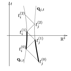
(a) The thick black stripes represent the initial data.

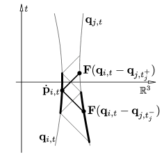
(b) Nature of the interaction.

Figure 1:

Definition 2.1.

We call a pair $\left(\mathbf{q}_{i}^{(0)},\mathbf{p}_{i}^{(0)}\right)_{i=1,2}$ of smooth position and momentum trajectory stripes

$$\mathbf{q}_{i}^{(0)}: \mathbb{R}\supset[t_{i}^{(0)},t_{i}^{(1)}] \to\mathbb{R}^{3},\qquad t\mapsto\mathbf{q}_{i,t}^{(0)},$$

$$\mathbf{p}_{i}^{(0)}: \mathbb{R}\supset[t_{i}^{(0)},t_{i}^{(1)}] \to\mathbb{R}^{3},\qquad t\mapsto\mathbf{p}_{i,t}^{(0)},\qquad i\in\{1,2\}$$

that fulfill the following conditions initial data for equation (6):

1. For times $t\in[t_{i}^{(0)},t_{i}^{(1)}]\cap[t_{j}^{(0)},t_{j}^{(1)}]$ it holds

   $$\mathbf{q}_{i,t}^{(0)}\neq\mathbf{q}_{j,t}^{(0)}.$$

2. For all $t\in[t_{i}^{(0)},t_{i}^{(1)}]$ it holds

   $$\frac{d}{dt}\mathbf{q}_{i,t}^{(0)}=\mathbf{v}(\mathbf{p}_{i,t}^{(0)})\equiv\frac{\mathbf{p}_{i,t}^{(0)}}{\sqrt{m_{i}^{2}+\left\|\mathbf{p}_{i,t}^{(0)}\right\|^{2}}},\qquad i\in\{1,2\}.$$ (8)

3. The times $t_{i}^{(0)},t_{i}^{(1)},t_{j}^{(0)},t_{j}^{(1)}$ relate to each other according to

   $$t_{i}^{(0)}=t_{i}^{+}\left(t_{j}^{(0)},\mathbf{q}_{j,t_{j}^{(0)}}^{(0)}\right),\qquad t_{j}^{(1)}=t_{j}^{+}\left(t_{i}^{(0)},\mathbf{q}_{i,t_{i}^{(0)}}^{(0)}\right),\qquad t_{i}^{(1)}=t_{i}^{+}\left(t_{j}^{(1)},\mathbf{q}_{j,t_{j}^{(1)}}^{(0)}\right).$$ (9)

4. At time $t=t_{i}^{(0)}$and for all integers $n\geq 0$ the trajectories obey

   $$\frac{d^{n}}{dt^{n}}\begin{pmatrix}\dot{\mathbf{q}}_{i,t}\\ \dot{\mathbf{p}}_{i,t}\end{pmatrix}=\frac{d^{n}}{dt^{n}}\begin{pmatrix}\mathbf{v}(\mathbf{p}_{i,t})\\ e_{i}e_{j}\left[\mathbf{F}\left(\mathbf{q}_{i,t}-\mathbf{q}_{j,t_{j}^{+}(t,\mathbf{q}_{i,t})}\right)+\mathbf{F}\left(\mathbf{q}_{i,t}-\mathbf{q}_{j,t_{j}^{-}(t,\mathbf{q}_{i,t})}\right)\right]\end{pmatrix}.$$ (10)

5. At time $t=t_{j}^{(1)}$and for all integers $n\geq 0$ the trajectories obey

   $$\frac{d^{n}}{dt^{n}}\begin{pmatrix}\dot{\mathbf{q}}_{j,t}\\ \dot{\mathbf{p}}_{j,t}\end{pmatrix}=\frac{d^{n}}{dt^{n}}\begin{pmatrix}\mathbf{v}(\mathbf{p}_{j,t})\\ e_{j}e_{i}\left[\mathbf{F}\left(\mathbf{q}_{j,t}-\mathbf{q}_{i,t_{i}^{+}(t,\mathbf{q}_{j,t})}\right)+\mathbf{F}\left(\mathbf{q}_{j,t}-\mathbf{q}_{i,t_{i}^{-}(t,\mathbf{q}_{j,t})}\right)\right]\end{pmatrix}.$$ (11)

Remark 2.2.

Note that (8) requires $\left\|\dot{\mathbf{q}}_{i,t}\right\|<1$ for $i\in\{1,2\}$ and

$$\mathbf{p}_{i,t}=\frac{m_{i}\dot{\mathbf{q}}_{i,t}}{\sqrt{1-\dot{\mathbf{q}}_{i,t}^{2}}}.$$

Furthermore, such initial data can be constructed as follows:

1. Choose times $t_{j}^{(0)}<t_{j}^{(1)}$, an arbitrary smooth trajectory strip $\mathbf{q}_{j}^{(0)}:[t_{j}^{(0)},t_{j}^{(1)}]\to\mathbb{R}^{3}$ with $\left\|\dot{\mathbf{q}}_{j,t}^{(0)}\right\|<1$, one space-point $(t_{i}^{(0)},\mathbf{q}_{i,t_{i}^{(0)}}^{(0)})$ on the intersection of the forward light-cone of $(t_{j}^{(0)},\mathbf{q}_{j,t_{j}^{(0)}}^{(0)})$ with the backward light-cone of $(t_{j}^{(1)},\mathbf{q}_{j,t_{j}^{(1)}}^{(0)})$, and one space-point $(t_{i}^{(1)},\mathbf{q}_{i,t_{i}^{(1)}}^{(0)})$ somewhere on the forward light-cone of $(t_{j}^{(1)},\mathbf{q}_{j,t_{j}^{(1)}}^{(0)})$ and inside the forward light-cone of $(t_{i}^{(0)},\mathbf{q}_{i,t_{i}^{(0)}}^{(0)})$.

2. Define $\mathbf{p}_{j,t}^{(0)}:=\frac{m_{j}\dot{\mathbf{q}}_{j,t}^{(0)}}{\sqrt{1-\dot{\mathbf{q}}_{j,t}^{2}}}$ for $t\in[t_{j}^{(0)},t_{j}^{(1)}]$ and, using (6), compute all derivatives of $\dot{\mathbf{p}}_{i,t}$ at the times $t=t_{i}^{(0)}$ and $t=t_{i}^{(1)}$.

3. Choose a smooth trajectory strip $\mathbf{q}_{i}^{(0)}:[t_{i}^{(0)},t_{i}^{(1)}]\to\mathbb{R}^{3}$ through the space-time points $(t_{i}^{(0)},\mathbf{q}_{i,t_{i}^{(0)}}^{(0)})$ and $(t_{i}^{(1)},\mathbf{q}_{i,t_{i}^{(1)}}^{(0)})$ such that $\left\|\dot{\mathbf{q}}_{j,t}^{(0)}\right\|<1$ and that $t\mapsto\mathbf{p}_{i,t}^{(0)}:=\frac{m_{i}\dot{\mathbf{q}}_{i,t}^{(0)}}{\sqrt{1-\left\|\dot{\mathbf{q}}_{i,t}\right\|^{2}}}$ smoothly connects to the derivatives computed in step 2.

Provided such initial data we shall prove our first result:

Theorem 2.3.

Given the initial data $\left(\mathbf{q}_{i}^{(0)},\mathbf{p}_{i}^{(0)}\right)_{i=1,2}$ there exist two smooth maps

$$\mathbb{R}\supseteq D_{i}\to\mathbb{R}^{3}\times\mathbb{R}^{3},\qquad t\mapsto(\mathbf{q}_{i,t},\mathbf{p}_{i,t}),\qquad i\in\{1,2\},$$ (12)

such that:

1. $(\mathbf{q}_{i,t},\mathbf{p}_{i,t})=(\mathbf{q}_{i,t}^{(0)},\mathbf{p}_{i,t}^{(0)})$ for all $t\in[t_{i}^{(0)},t_{i}^{(1)}]$ and $i\in\{1,2\}$.

2. $t\mapsto(\mathbf{q}_{i,t},\mathbf{p}_{i,t})$ solves (6) on $D_{i}:=\left(t_{i}^{+}(T_{j}^{\min},\mathbf{q}_{j,T_{j}^{\min}}),t_{i}^{-}(T_{j}^{\max},\mathbf{q}_{j,T_{j}^{\max}})\right)$ for $i\in\{1,2\}$, $j\neq i$.

3. For $i=1,2$ let $\widetilde{D}_{i}\subseteq\mathbb{R}$ be an interval such that $[t_{i}^{(0)},t_{i}^{(1)}]\subseteq\widetilde{D}_{i}$ and let $\widetilde{D}_{i}\to\mathbb{R}^{3}\times\mathbb{R}^{3}$, $t\mapsto(\widetilde{\mathbf{q}}_{i,t},\widetilde{\mathbf{p}}_{i,t})$ be a smooth map such that $t\mapsto(\widetilde{\mathbf{q}}_{i,t},\widetilde{\mathbf{p}}_{i,t})$ solves (6) for $t\in\widetilde{D}_{i}$. Then:

   $$(\widetilde{\mathbf{q}}_{i,t},\widetilde{\mathbf{p}}_{i,t})=(\mathbf{q}_{i,t},\mathbf{p}_{i,t})\,\forall t\in D_{i}\cap\widetilde{D}_{i},i\in\{1,2\}$$

   $$\Updownarrow$$

   $$(\widetilde{\mathbf{q}}_{i,t},\widetilde{\mathbf{p}}_{i,t})=(\mathbf{q}_{i,t},\mathbf{p}_{i,t})\,\forall t\in[t_{i}^{(0)},t_{i}^{(1)}],i\in\{1,2\}.$$

Given appropriate constants $d>0$ and $0\leq v<1$, the times $-\infty\leq T_{i}^{\min}\leq t_{i}^{(0)}<t_{i}^{(1)}\leq T_{i}^{\max}\leq\infty$ are defined such that $[T_{i}^{\min},T_{i}^{\max}]$ is the largest interval containing $[t_{i}^{(0)},t_{i}^{(1)}]$ with the property:

$$\left\|\dot{\mathbf{q}}_{i,t}\right\|\leq v,\qquad\left\|\mathbf{q}_{i,t}-\mathbf{q}_{j,t_{j}^{\pm}(t,\mathbf{q}_{i,t})}\right\|\geq d,\qquad\forall\,t\in[T_{i}^{\min},T_{i}^{\max}]$$ (13)

Their value is determined during the construction of (12) in the proof.

Remark 2.4.

Our focus lies on the uniqueness assertion (iii) of 2.3. We do not attempt to give a priori bounds on $T_{i}^{\min},T_{i}^{\max}$, $i\in\{1,2\}$, whose values are determined during the dynamics by condition (13). This condition is needed to prevent two types of singularities that can occur: First, the approach of the speed of light, and second, collision or infinitesimal approach of charges. These singularities can also be present in WF which can be seen directly from the form of the fields (2). While the second one is familiar since it is of the same type as seen in the $N$-body problem of Newtonian gravitation [SMSM71], the first one is very specific to WF-type delay problems. Such singularities are due to the nature of the delay times $t_{j}^{+}$ and $t_{j}^{-}$ defined in (4) which tend to plus or minus infinity if the $j$-th charge approaches the speed of light in the future or the past, respectively; the origin of this singularity can be seen best in (18). Because of angular momentum conservation it is however expected that for $N=2$ charges one always finds $T_{\min}=-\infty$ and $T_{\max}=\infty$, which is at least true for the solutions given in 4. A treatment of the $N$-body problem will require a notion of typicality of solutions.

The key ingredient of the proof, which can be checked by direct computation, is the following:

Lemma 2.5.

The following statements are true:

1. The map $\mathbf{F}$ defined in (7) is bijective and its inverse is given by

   $$\mathbf{I}:\mathbb{R}^{3}\setminus\{0\}\to\mathbb{R}^{3}\setminus\{0\},\qquad\mathbf{y}\mapsto\mathbf{I}(\mathbf{y}):=\frac{\mathbf{y}}{\left\|\mathbf{y}\right\|^{3/2}}.$$

2. Let $\left(\mathbf{q}_{i}^{(0)},\mathbf{p}_{i}^{(0)}\right)_{i=1,2}$ be given initial data. For any integer $n\geq 0$ equations (10) and (11) are equivalent to

   $$\frac{d^{n}}{dt^{n}}\left(\mathbf{q}_{i,t}-\mathbf{q}_{j,t_{j}^{\pm}(t,\mathbf{q}_{i,t})}\right)=\frac{d^{n}}{dt^{n}}\mathbf{I}\left(\frac{1}{e_{i}e_{j}}\dot{\mathbf{p}}_{i,t}-\mathbf{F}\left(\mathbf{q}_{i,t}-\mathbf{q}_{j,t_{j}^{\mp}(t,\mathbf{q}_{i,t})}\right)\right)\qquad\text{for }t=t_{i}^{(0)},$$

   and

   $$\frac{d^{n}}{dt^{n}}\left(\mathbf{q}_{j,t}-\mathbf{q}_{i,t_{i}^{\pm}(t,\mathbf{q}_{j,t})}\right)=\frac{d^{n}}{dt^{n}}\mathbf{I}\left(\frac{1}{e_{j}e_{i}}\dot{\mathbf{p}}_{j,t}-\mathbf{F}\left(\mathbf{q}_{j,t}-\mathbf{q}_{i,t_{i}^{\mp}(t,\mathbf{q}_{j,t})}\right)\right)\qquad\text{for }t=t_{j}^{(0)},$$

   respectively.

2.5 ensures that for example in situations as depicted in 1b we can compute from $\mathbf{F}(\mathbf{q}_{i,t}-\mathbf{q}_{j,t_{j}^{+}})$, which is determined by the initial data and (6), the space-time point $(t_{j}^{+},\mathbf{q}_{j,t_{j}^{+}})$. This is the key ingredient in our construction:

Proof of 2.3.

As a first step, we construct a smooth extension of $\mathbf{q}_{j}^{(0)}$ beyond time $t_{j}^{(1)}$. Let us introduce the short-hand notation

$$t_{j}^{\pm}=t_{j}^{\pm}(t,\mathbf{q}_{i,t}).$$

In general, any solution $t\mapsto(\mathbf{q}_{i,t},\mathbf{p}_{i,t})_{i=1,2}$ to (6) has to fulfill

$$\dot{\mathbf{p}}_{i,t}=e_{i}e_{j}\left[\mathbf{F}\left(\mathbf{q}_{i,t}-\mathbf{q}_{j,t_{j}^{+}}\right)+\mathbf{F}\left(\mathbf{q}_{i,t}-\mathbf{q}_{j,t_{j}^{-}}\right)\right].$$ (14)

With the help of 2.5(i) we can bring this equation into the form

$$\mathbf{q}_{j,t_{j}^{+}}=\mathbf{q}_{i,t}-\mathbf{I}\left(\frac{1}{e_{i}e_{j}}\dot{\mathbf{p}}_{i,t}-\mathbf{F}\left(\mathbf{q}_{i,t}-\mathbf{q}_{j,t_{j}^{\mp}(t,\mathbf{q}_{i,t})}\right)\right)$$ (15)

for times $t\in[T_{i}^{\min},T_{i}^{\max}]$ because then

$$\left\|\mathbf{I}\left(\frac{1}{e_{i}e_{j}}\dot{\mathbf{p}}_{i,t}-\mathbf{F}\left(\mathbf{q}_{i,t}-\mathbf{q}_{j,t_{j}^{-}}\right)\right)\right\|=\left\|\mathbf{q}_{i,t}-\mathbf{q}_{j,t_{j}^{\pm}}\right\|\geq d$$

is guaranteed, and hence, the right-hand side of (15) is well-defined. We now make use of (15) to compute

$$\mathbf{q}_{j}^{(1)}:t\mapsto\mathbf{q}_{j,t}^{(1)}$$

according to

$$t_{j}^{+} = t+\left\|\mathbf{I}\left(\frac{1}{e_{i}e_{j}}\dot{\mathbf{p}}_{i,t}^{(0)}-\mathbf{F}\left(\mathbf{q}_{i,t}^{(0)}-\mathbf{q}_{j,t_{j}^{-}(t,\mathbf{q}_{i,t})}^{(0)}\right)\right)\right\|,$$ (16)

$$\mathbf{q}_{j,t_{j}^{+}}^{(1)} = \mathbf{q}_{i,t}^{(0)}-\mathbf{I}\left(\frac{1}{e_{i}e_{j}}\dot{\mathbf{p}}_{i,t}^{(0)}-\mathbf{F}\left(\mathbf{q}_{i,t}^{(0)}-\mathbf{q}_{j,t_{j}^{-}(t,\mathbf{q}_{i,t})}^{(0)}\right)\right)$$ (17)

for all $t\in(t_{i}^{(0)},t_{i}^{(1)}]\cap(T_{i}^{\min},T_{i}^{\max})$. Note that due to (9) the right-hand side of (16) and (17) is well-defined. We define

$$t_{j}^{(2)}=\min\left\{t_{j}^{+}|_{t=t_{i}^{(1)}},T_{j}^{\max}\right\}.$$

Since $\mathbf{q}_{i}^{(0)}$ is smooth on $[t_{i}^{(0)},t_{i}^{(1)}]$ also $t_{j}^{+}$ depends smoothly on $t\in[t_{i}^{(0)},t_{i}^{(1)}]$, and in consequence, $\mathbf{q}_{j}^{(1)}$ is smooth on $(t_{j}^{(1)},t_{j}^{(2)}]$. Furthermore, a direct computation gives

$$t\mapsto\frac{dt_{j}^{+}}{dt}=\frac{1+\mathbf{n}_{j,+}\cdot\dot{\mathbf{q}}_{i,t}^{(0)}}{1+\mathbf{n}_{j,+}\cdot\dot{\mathbf{q}}_{j,t^{+}}^{(1)}},\qquad\mathbf{n}_{j,+}:=\frac{\mathbf{\mathbf{q}}_{i,t}^{(0)}-\mathbf{q}_{j,t^{+}}^{(1)}}{\left\|\mathbf{\mathbf{q}}_{i,t}^{(0)}-\mathbf{q}_{j,t^{+}}^{(1)}\right\|}.$$ (18)

so that, using the notation

$$\frac{d}{dt_{j}^{+}}=\frac{dt}{dt_{j}^{+}}\frac{d}{dt},$$

we may then compute

$$\lim_{s\searrow t_{j}^{(1)}}\frac{d^{n}}{ds^{n}}\mathbf{q}_{j,s}^{(1)} = \lim_{t\searrow t_{i}^{(0)}}\frac{d^{n}}{dt_{j}^{+n}}\mathbf{q}_{j,t_{j}^{+}}^{(1)}=\lim_{t\searrow t_{i}^{(0)}}\frac{d^{n}}{dt_{j}^{+n}}\left[\mathbf{q}_{i,t}^{(0)}-\mathbf{I}\left(\frac{1}{e_{i}e_{j}}\dot{\mathbf{p}}_{i,t}^{(0)}-\mathbf{F}\left(\mathbf{q}_{i,t}^{(0)}-\mathbf{q}_{j,t_{j}^{-}(t,\mathbf{q}_{i,t})}^{(1)}\right)\right)\right]$$ (19)

for every integer $n\geq 0$. 2.5(ii) ensures that

$$(\ref{eq:check smoothness})=\frac{d^{n}}{ds^{n}}\mathbf{q}_{j,s}^{(0)}\big{|}_{s=t_{j}^{(1)}},$$

and hence,

$$t\mapsto\begin{cases}\mathbf{q}_{j,t}^{(0)}&\text{for }t\in[t_{j}^{(0)},t_{j}^{(1)}]\\ \mathbf{q}_{j,t}^{(1)}&\text{for }t\in(t_{j}^{(1)},t_{j}^{(2)}]\end{cases}$$

is a smooth map on $[t_{j}^{(0)},t_{j}^{(2)})$. Furthermore,

$$\mathbf{p}_{j,t}^{(1)}:=m\frac{\dot{\mathbf{q}}_{j,t}}{\sqrt{1-\dot{\mathbf{q}}_{j,t}^{2}}},\qquad\forall\,t\in(t_{j}^{(1)},t_{j}^{(2)}].$$ (20)

is well-defined by (13).

In the second step, we use the analogous construction to extend $\mathbf{q}_{i}^{(0)}$ smoothly beyond time $t_{i}^{(1)}$: We define

$$\mathbf{q}_{i}^{(1)}:t\mapsto\mathbf{q}_{i,t}^{(1)}$$

by

$$t_{i}^{+} = t+\left\|\mathbf{q}_{j,t}^{(1)}-\mathbf{I}\left(\frac{1}{e_{j}e_{i}}\dot{\mathbf{p}}_{j,t}^{(1)}-\mathbf{F}\left(\mathbf{q}_{j,t}^{(1)}-\mathbf{q}_{i,t_{i}^{-}(t,\mathbf{q}_{j,t})}^{(0)}\right)\right)\right\|,$$ (21)

$$\mathbf{q}_{i,t_{i}^{+}}^{(1)} = \mathbf{q}_{j,t}^{(1)}-\mathbf{I}\left(\frac{1}{e_{j}e_{i}}\dot{\mathbf{p}}_{j,t}^{(1)}-\mathbf{F}\left(\mathbf{q}_{j,t}^{(1)}-\mathbf{q}_{i,t_{i}^{-}(t,\mathbf{q}_{j,t})}^{(0)}\right)\right)$$ (22)

for all $t\in(t_{j}^{(1)},t_{j}^{(2)}]\cap[T_{j}^{\min},T_{j}^{\max}]$ and furthermore

$$t_{i}^{(2)}=\min\left\{t_{i}^{+}|_{t=t_{j}^{(2)}},T_{i}^{\max}\right\}.$$

As in the first step one finds that

$$t\mapsto\begin{cases}\mathbf{q}_{i,t}^{(0)}&\text{for }t\in[t_{i}^{(0)},t_{i}^{(1)}]\\ \mathbf{q}_{i,t}^{(1)}&\text{for }t\in(t_{i}^{(1)},t_{i}^{(2)}]\end{cases}$$

is smooth for $t\in[t_{i}^{(0)},t_{i}^{(2)}]$. Finally, due to (13) we can define

$$\mathbf{p}_{i,t}^{(1)}:=m\frac{\dot{\mathbf{q}}_{i,t}}{\sqrt{1-\dot{\mathbf{q}}_{i,t}^{2}}},\qquad\forall\,t\in(t_{i}^{(1)},t_{i}^{(2)}].$$ (23)

In consequence, the maps

$$t\mapsto(\mathbf{q}_{i,t},\mathbf{p}_{i,t}):=\begin{cases}(\mathbf{q}_{i,t}^{(0)},\mathbf{p}_{i,t}^{(0)})&\text{for }t\in[t_{i}^{(0)},t_{i}^{(1)}]\\ (\mathbf{q}_{i,t}^{(0)},\mathbf{p}_{i,t}^{(0)})&\text{for }t\in(t_{i}^{(1)},t_{i}^{(2)}]\end{cases}$$

for $i=1,2$ are smooth, and by virtue of definitions (20),(23) and (17), (22) and (10),(11) of (2.5) they fulfill

$$\begin{pmatrix}\mathbf{q}_{i,t}\\ \mathbf{p}_{i,t}\end{pmatrix}=\begin{pmatrix}\mathbf{v}(\mathbf{p}_{i,t})\\ e_{i}e_{j}\left[\mathbf{F}\left(\mathbf{q}_{i,t}-\mathbf{q}_{j,t_{j}^{+}}\right)+\mathbf{F}\left(\mathbf{q}_{i,t}-\mathbf{q}_{j,t_{j}^{-}}\right)\right]\end{pmatrix}$$ (24)

for $t\in[t_{i}^{(0)},t_{i}^{-}(t_{j}^{(2)},\mathbf{q}_{j,t_{j}^{(2)}})]$ and

$$\begin{pmatrix}\mathbf{q}_{j,t}\\ \mathbf{p}_{j,t}\end{pmatrix}=\begin{pmatrix}\mathbf{v}(\mathbf{p}_{j,t})\\ e_{j}e_{i}\left[\mathbf{F}\left(\mathbf{q}_{j,t}-\mathbf{q}_{i,t_{i}^{+}}\right)+\mathbf{F}\left(\mathbf{q}_{j,t}-\mathbf{q}_{i,t_{i}^{-}}\right)\right]\end{pmatrix}$$ (25)

for $t\in[t_{j}^{(1)},t_{j}^{-}(t_{i}^{(2)},\mathbf{q}_{i,t_{i}^{(2)}})].$

This construction can be repeated where in the $k$th step one constructs the extension

$$(t_{i}^{(k)},t_{i}^{(k+1)}]:t\mapsto(\mathbf{q}_{i,t}^{(k)},\mathbf{p}_{i,t}^{(k)})_{i=1,2}.$$

For each step one finds

$$t_{i}^{(k+1)}\geq\min\left\{t^{(k)}+d,T_{i}^{\max}\right\},\qquad i\in\{1,2\}.$$

In consequence, only finite repetitions of this construction are needed to compute

$$[t_{i}^{(0)},T_{i}^{\max}]:t\mapsto(\mathbf{q}_{i,t},\mathbf{p}_{i,t}):=\begin{cases}(\mathbf{q}_{i,t}^{(0)},\mathbf{p}_{i,t}^{(0)})&\text{for }t\in[t_{i}^{(0)},t_{i}^{(1)}]\\ (\mathbf{q}_{i,t}^{(k)},\mathbf{p}_{i,t}^{(k)})&\text{for }t\in(t_{i}^{(k)},t_{i}^{(k+1)}]\end{cases}$$ (26)

which fulfills (24) for $t\in[t_{i}^{(0)},t_{i}^{-}(T_{j}^{\max},\mathbf{q}_{j,T_{j}^{\max}})]$ and (25) for $t\in[t_{j}^{(1)},t_{j}^{-}(T_{i}^{\max},\mathbf{q}_{i,T_{i}^{\max}})]$. The same construction can be carried out into the past which results in smooth maps

$$[T_{i}^{\min},T_{i}^{\max}]\to\mathbb{R}^{3}\times\mathbb{R}^{3},\qquad t\mapsto(\mathbf{q}_{i,t},\mathbf{p}_{i,t}),\qquad i\in\{1,2\}.$$

From this construction we infer the claims of 2.3: Claim (i) follows from definition (26). Furthermore, due to 2.5, (16)-(17) and (21)-(22) the map $t\mapsto(\mathbf{q}_{i,t},\mathbf{p}_{i,t})$ fulfills (6) for times

$$t\in[t_{i}^{+}(T_{j}^{\min},\mathbf{q}_{j,T_{j}^{\min}}),t_{i}^{-}(T_{j}^{\max},\mathbf{q}_{j,T_{j}^{\max}})]$$

for $i\in\{1,2\}$ and $j\neq i$ and therefore claim (ii). Finally, 2.5 guarantees that this constructed solution is unique which proves claim (iii) and concludes the proof. ∎

As a byproduct we observe that specification of initial positions and momenta of the charges as suggested by the work [Dri79] does not always ensure uniqueness:

Corollary 2.6.

Let $\left(\mathbf{q}_{i}^{(0)},\mathbf{p}_{i}^{(0)}\right)_{i=1,2}$ be initial data such that there is a $t^{*}\in(t_{i}^{(0)},t_{i}^{(1)})\cap(t_{j}^{(0)},t_{j}^{(1)})$, let $D_{i}\to\mathbb{R}^{3}\times\mathbb{R}^{3},t\mapsto(\mathbf{q}_{i,t},\mathbf{p}_{i,t})$ for $i\in\{1,2\}$ be the corresponding solution to (6), and let $\mathbf{q}_{i}^{(0)},\mathbf{p}_{i}^{(0)}\in\mathbb{R}^{3}$ for $i=1,2$ be defined as

$$(\mathbf{q}_{i}^{(0)},\mathbf{p}_{i}^{(0)}):=(\mathbf{q}_{i,t},\mathbf{p}_{i,t})\big{|}_{t=t^{*}},\qquad i\in\{1,2\}.$$

There are uncountably many other solutions $\widetilde{D}_{i}\to\mathbb{R}^{3}\times\mathbb{R}^{3},t\mapsto(\widetilde{\mathbf{q}}_{i,t},\widetilde{\mathbf{p}}_{i,t})$ for $i=1,2$ to (6) which fulfill

$$(\widetilde{\mathbf{q}}_{i,t},\widetilde{\mathbf{p}}_{i,t})\big{|}_{t=t^{*}}=(\mathbf{q}_{i}^{(0)},\mathbf{p}_{i}^{(0)}),\qquad i\in\{1,2\},$$ (27)

but not

$$(\widetilde{\mathbf{q}}_{i,t},\widetilde{\mathbf{p}}_{i,t})=(\mathbf{q}_{i,t},\mathbf{p}_{i,t})\qquad\forall\,t\in D_{i}\cap\widetilde{D}_{i},\quad i\in\{1,2\}.$$ (28)

Proof.

Choose $s\in\mathbb{R}$ and $\delta>0$ such that $(s-\delta,s+\delta)\subset(t_{i}^{(0)},t_{i}^{(1)})\cap(t_{j}^{(0)},t_{j}^{(1)})$ and $t^{*}\notin(s-\delta,s+\delta)$. Furthermore, for $\lambda>0$ and $i=1,2$ let $\mathbf{d}_{\lambda,i}:\mathbb{R}\to\mathbb{R}^{3}$, $t\mapsto\mathbf{d}_{\lambda,i}(t)$ be a smooth function such that

$$\mathrm{supp}\,\mathbf{d}_{\lambda,i}=[s-\delta,s+\delta],\qquad\sup_{t\in\mathbb{R}}|\dot{\mathbf{d}}_{\lambda,i}(t)|=\lambda.$$

We define

$$t\mapsto\widetilde{\mathbf{q}}_{i,t}^{(0)}:=\mathbf{q}_{i,t}^{(0)}+\mathbf{d}_{\lambda,i}(t),\qquad\forall\,t\in[t_{i}^{(0)},t_{i}^{(1)}],$$

choose the parameter $\lambda>0$ such that $\left\|\dot{\widetilde{\mathbf{q}}}_{i,t}\right\|<1$, and define

$$t\mapsto\widetilde{\mathbf{p}}_{i,t}^{(0)}:=\frac{m_{i}\dot{\widetilde{\mathbf{q}}}_{i,t}}{\sqrt{1-\left\|\dot{\widetilde{\mathbf{q}}}_{i,t}\right\|^{2}}},\qquad\forall\,t\in[t_{i}^{(0)},t_{i}^{(1)}].$$

The maps $(\widetilde{\mathbf{q}}_{i}^{(0)},\widetilde{\mathbf{p}}_{i}^{(0)})_{i=1,2}$ are initial data according to 2.1 which fulfill (27). However, according to 2.3 the solution $\widetilde{D}_{i}\to\left(\mathbb{R}^{3}\times\mathbb{R}^{3}\right),t\mapsto(\widetilde{\mathbf{q}}_{i,t},\widetilde{\mathbf{p}}_{i,t})$ for $i=1,2$ to (6) corresponding to $(\widetilde{\mathbf{q}}_{i}^{(0)},\widetilde{\mathbf{p}}_{i}^{(0)})_{i=1,2}$ does not fulfill (28). Note that there are uncountably many choices, e.g. in $s,\delta,\lambda$ and $\mathbf{d}_{\lambda,i}$, to define other $(\widetilde{\mathbf{q}}_{i}^{(0)},\widetilde{\mathbf{p}}_{i}^{(0)})_{i=1,2}$ such that (27) holds. None of the corresponding solutions however fulfill (28). ∎

3 Constants of Motion

In the following we define an energy functional for the approximate model from which the general structure of constants of motion will become apparent. Throughout this section we consider a solution

$$\mathbb{R}\supseteq D_{i}\to\mathbb{R}^{3}\times\mathbb{R}^{3},\qquad t\mapsto(\mathbf{q}_{i,t},\mathbf{p}_{i,t}),\qquad i\in\{1,2\},$$

to (6); see 2.3.

Definition 3.1.

We define a map $H:D_{1}\times D_{2}\to\mathbb{R}^{+}$ by

$$H(t_{1},t_{2}): = \sum_{i=1}^{2}\sqrt{\mathbf{p}_{i,t_{i}}^{2}+m_{i}^{2}}+\frac{1}{2}\sum_{i=1}^{2}e_{i}\sum_{j\neq i}e_{j}\sum_{\pm}\frac{1}{\left\|\mathbf{q}_{i,t_{i}}-\mathbf{q}_{j,t_{j}^{\pm}(t_{i})}\right\|}$$

$$+\frac{1}{2}\sum_{i=1}^{2}e_{i}\sum_{j\neq i}e_{j}\sum_{\pm}\int_{t_{i}}^{t_{i}^{\pm}(t_{j})}ds\,\mathbf{F}(\mathbf{q}_{i,s}-\mathbf{q}_{j,t_{j}^{\pm}(s)})\cdot\dot{\mathbf{q}}_{i,s}$$

where for the delay functions we have used the short-hand notation

$$t_{i}^{\pm}(t)\equiv t_{i}^{\pm}(t,\mathbf{q}_{j,t}),\qquad i\in\{1,2\},\quad j\neq i.$$

We refer to $H$ as the energy functional of the system. See 2 for an example of which data is needed to define this functional.

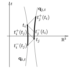
Figure 2: Given $t_{i},t_{j}$ the thick lines denote the data required to define the energy of the system.

Theorem 3.2.

For all $t_{1}\in D_{1}$ and $t_{2}\in D_{2}$ the equality

$$H(t_{1},t_{2})=H(0,0)$$

holds true.

Proof.

Since we assume a smooth solution $t\mapsto(\mathbf{q}_{i,t},\mathbf{p}_{i,t})_{i=1,2}$ to (6) it is straight-forward to verify the claim directly by differentiating with respect to $t_{1}$ and $t_{2}$. Here, however, we want to provide a general idea how to find constants of motion for a WF-type delay differential equations, and therefore give a more instructive proof:

We start with the sum of the kinetic energy difference between times $0$ and $t_{i}$ of the two particles $i=1,2$, that is

$$\sum_{i=1}^{2}\int_{0}^{t_{i}}ds\,\dot{\mathbf{p}}_{i,s}\cdot\mathbf{v}(\mathbf{p}_{i,s})$$ (29)

and make use of the equations (6) to express this entity in terms of

$$(\ref{eq:kinetic})=\sum_{i=1}^{2}e_{i}\sum_{j\neq i}e_{j}\sum_{\pm}\int_{0}^{t_{i}}ds\,\mathbf{F}(\mathbf{q}_{i,s}-\mathbf{q}_{j,t_{j}^{\pm}(s)})\cdot\dot{\mathbf{q}}_{i,s}.$$ (30)

It is convenient to split (30) into the following summands:

$$(\ref{eq:kinetic2}) = \frac{1}{2}\sum_{i=1}^{2}e_{i}\sum_{j\neq i}e_{j}\sum_{\pm}\int_{0}^{t_{i}}ds\,\mathbf{F}(\mathbf{q}_{i,s}-\mathbf{q}_{j,t_{j}^{\pm}(s)})\cdot\dot{\mathbf{q}}_{i,s}$$ (33)

$$+\frac{1}{2}\sum_{i=1}^{2}e_{i}\sum_{j\neq i}e_{j}\sum_{\pm}\int_{0}^{t_{i}}ds\,\mathbf{F}(\mathbf{q}_{i,s}-\mathbf{q}_{j,t_{j}^{\pm}(s)})\cdot\left(\dot{\mathbf{q}}_{i,s}-\dot{\mathbf{q}}_{j,t_{j}^{\pm}(s)}\frac{dt_{j}^{\pm}(s)}{ds}\right)$$

$$+\frac{1}{2}\sum_{i=1}^{2}e_{i}\sum_{j\neq i}e_{j}\sum_{\pm}\int_{0}^{t_{i}}ds\,\mathbf{F}(\mathbf{q}_{i,s}-\mathbf{q}_{j,t_{j}^{\pm}(s)})\cdot\dot{\mathbf{q}}_{j,t_{j}^{\pm}(s)}\frac{dt_{j}^{\pm}(s)}{ds}.$$

The integrand in (33) is an exact differential so that

$$(\ref{eq:potential})=-\frac{1}{2}\sum_{i=1}^{2}e_{i}\sum_{j\neq i}e_{j}\sum_{\pm}\frac{1}{\left\|\mathbf{q}_{i,t_{i}}-\mathbf{q}_{j,t_{j}^{\pm}(t_{i})}\right\|}+C$$ (34)

where $C\in\mathbb{R}$ is a constant. Next, we exploit the symmetries of the force field and the delay function

$$\mathbf{F}(\mathbf{x})=-\mathbf{F}(\mathbf{x}),\qquad\forall\,\mathbf{x}\in\mathbb{R}^{3}\setminus\{0\},$$ (35)

$$t=t_{i}^{\mp}\left(t_{j}^{\pm}(t)\right),\qquad i\in\{1,2\},\quad j\neq i.$$ (36)

Now (36) allows to rewrite (33) by substitution of the integration variable according to

$$(\ref{eq:functional})=\frac{1}{2}\sum_{i=1}^{2}e_{i}\sum_{j\neq i}e_{j}\sum_{\pm}\int_{t_{j}^{\pm}(0)}^{t_{j}^{\pm}(t_{i})}ds\,\mathbf{F}(\mathbf{q}_{i,t_{i}^{\mp}(s)}-\mathbf{q}_{j,s})\cdot\dot{\mathbf{q}}_{j,s}.$$ (37)

Furthermore, we apply (35) and after that relabel the indices $i\leftrightarrows j$ and $\pm\leftrightarrows\mp$ to get

$$(\ref{eq:subst}) =- \frac{1}{2}\sum_{i=1}^{2}e_{i}\sum_{j\neq i}e_{j}\sum_{\pm}\int_{t_{j}^{\pm}(0)}^{t_{j}^{\pm}(t_{i})}ds\,\mathbf{F}(\mathbf{q}_{j,s}-\mathbf{q}_{i,t_{i}^{\mp}(s)})\cdot\dot{\mathbf{q}}_{j,s}$$ (40)

$$=- \frac{1}{2}\sum_{i=1}^{2}e_{i}\sum_{j\neq i}e_{j}\sum_{\pm}\int_{t_{i}^{\mp}(0)}^{t_{i}^{\mp}(t_{j})}ds\,\mathbf{F}(\mathbf{q}_{i,s}-\mathbf{q}_{j,t_{j}^{\pm}(s)})\cdot\dot{\mathbf{q}}_{i,s}$$

$$=- \frac{1}{2}\sum_{i=1}^{2}e_{i}\sum_{j\neq i}e_{j}\sum_{\pm}\int_{t_{i}^{\pm}(0)}^{0}ds\,\mathbf{F}(\mathbf{q}_{i,s}-\mathbf{q}_{j,t_{j}^{\pm}(s)})\cdot\dot{\mathbf{q}}_{i,s}$$

$$-\frac{1}{2}\sum_{i=1}^{2}e_{i}\sum_{j\neq i}e_{j}\sum_{\pm}\int_{0}^{t_{i}}ds\,\mathbf{F}(\mathbf{q}_{i,s}-\mathbf{q}_{j,t_{j}^{\pm}(s)})\cdot\dot{\mathbf{q}}_{i,s}$$

$$-\frac{1}{2}\sum_{i=1}^{2}e_{i}\sum_{j\neq i}e_{j}\sum_{\pm}\int_{t_{i}}^{t_{i}^{\mp}(t_{j})}ds\,\mathbf{F}(\mathbf{q}_{i,s}-\mathbf{q}_{j,t_{j}^{\pm}(s)})\cdot\dot{\mathbf{q}}_{i,s}$$

Noting that term (40) is just another constant and term (40) cancels the first term on the right-hand side of (33), the kinetic energy can be written as

$$(\ref{eq:kinetic})=-\frac{1}{2}\sum_{i=1}^{2}e_{i}\sum_{j\neq i}e_{j}\sum_{\pm}\frac{1}{\left\|\mathbf{q}_{i,t_{i}}-\mathbf{q}_{j,t_{j}^{\pm}(t_{i})}\right\|}-\frac{1}{2}\sum_{i=1}^{2}e_{i}\sum_{j\neq i}e_{j}\sum_{\pm}\int_{t_{i}}^{t_{i}^{\mp}(t_{j})}ds\,\mathbf{F}(\mathbf{q}_{i,s}-\mathbf{q}_{j,t_{j}^{\pm}(s)})\cdot\dot{\mathbf{q}}_{i,s}+C$$

which proves the claim. ∎

4 Stable Orbits

By the symmetry of the advanced and retarded delay it is straight-forward to construct stable orbits (compare [Sch63]):

Definition 4.1.

For masses $m_{1},m_{2}>0$, charges $e_{1},e_{2}\in\mathbb{R}$, radii $r_{1},r_{2}>0$, and angular velocity $\omega\in\mathbb{R}\setminus\{0\}$ such that

$$e_{1}e_{2}<0,\qquad\frac{m_{1}}{m_{2}}=\frac{\gamma(\omega r_{2})}{\gamma(\omega r_{1})}\frac{r_{2}}{r_{1}},\qquad 0<\omega\Delta T<\frac{\pi}{2},\qquad\Delta T:=\sqrt{\frac{r_{1}^{2}+r_{2}^{2}}{1+\frac{r_{1}r_{2}}{e_{1}e_{2}}m_{1}\gamma(\omega r_{1})r_{1}\omega^{2}}},$$

where

$$\gamma(v):=\frac{1}{\sqrt{1-v^{2}}},$$

we define the particle trajectories

$$t\mapsto\mathbf{q}_{1,t}:=r_{1}\begin{pmatrix}\cos\omega t\\ \sin\omega t\end{pmatrix},\qquad t\mapsto\mathbf{q}_{2,t}:=-r_{2}\begin{pmatrix}\cos\omega t\\ \sin\omega t\end{pmatrix}$$ (41)

which we call Schild solutions; see 3.

Theorem 4.2.

Given $m_{1,}m_{2},r_{1}>0$, $e_{1}\in\mathbb{R}$ there are $r_{2}>0$ and $\omega\in\mathbb{R}$ such that the Schild solutions (41) obey (6).

Figure 3: Stable orbit of two charges revolving around the same center with radii $r_{i},r_{j}$. $\Delta T$ denotes the modulus of the delay.

Proof.

We start by rewriting (6) as a second order equation, i.e.

$$\frac{d}{dt}\left(m_{i}\gamma(\dot{\mathbf{q}}_{i,t})\dot{\mathbf{q}}_{i,t}\right)=e_{i}e_{j}\left[\mathbf{F}\left(\mathbf{q}_{i,t}-\mathbf{q}_{j,t_{j}^{+}(t,\mathbf{q}_{i,t})}\right)+\mathbf{F}\left(\mathbf{q}_{i,t}-\mathbf{q}_{j,t_{j}^{-}(t,\mathbf{q}_{i,t})}\right)\right],\qquad i\in\{1,2\},\quad i\neq j.$$

If the charges stay on the circular orbits (41) then velocities and accelerations are constant and fulfill

$$\left\|\dot{\mathbf{q}}_{i,t}\right\|=\omega r_{i},\qquad\left\|\ddot{\mathbf{q}}_{i,t}\right\|=\omega^{2}r_{i}.$$

Furthermore, the kinematics dictate that the net force acting upon the particles must be centripetal w.r.t. the origin and equal, i.e.

$$\left\|\frac{d}{dt}\left(m_{1}\gamma(\dot{\mathbf{q}}_{1,t})\dot{\mathbf{q}}_{1,t}\right)\right\|=m_{1}\gamma(\omega r_{1})\omega^{2}r_{1}=m_{2}\gamma(\omega r_{2})\omega^{2}r_{2}$$

which implies

$$\frac{m_{1}}{m_{2}}=\frac{\gamma(\omega r_{2})}{\gamma(\omega r_{1})}\frac{r_{2}}{r_{1}}.$$ (42)

Next, we compute the delay function $\Delta T>0$ which, according to (4), was defined by

$$\Delta T^{2}:=\left(t_{j}^{\pm}(t)-t\right)^{2}=\left\|\mathbf{q}_{i,t}-\mathbf{q}_{j,t_{j}^{\pm}(t)}\right\|^{2}=r_{1}^{2}+r_{2}^{2}+2r_{1}r_{2}\cos\left(\omega\Delta T\right).$$ (43)

Due to the symmetry in the advanced and retarded delay (see 3) the net force is centripetal w.r.t. the origin for

$$e_{1}e_{2}<0$$

and its modulus equals

$$\left\|e_{i}e_{j}\left[\mathbf{F}\left(\mathbf{q}_{i,t}-\mathbf{q}_{j,t_{j}^{+}(t,\mathbf{q}_{i,t})}\right)+\mathbf{F}\left(\mathbf{q}_{i,t}-\mathbf{q}_{j,t_{j}^{-}(t,\mathbf{q}_{i,t})}\right)\right]\right\|=\left|e_{1}e_{2}\frac{2\cos\left(\omega\Delta T\right)}{\Delta T^{2}}\right|.$$

This means in particular that

$$m_{1}\gamma(\omega r_{1})\omega^{2}r_{1}=\left|e_{1}e_{2}\frac{2\cos\left(\omega\Delta T\right)}{\Delta T^{2}}\right|$$

which by (4) allows to solve for $\Delta T$ according to

$$\Delta T^{2}=\frac{r_{1}^{2}+r_{2}^{2}}{1+\frac{r_{1}r_{2}}{e_{1}e_{2}}m_{1}\gamma(\omega r_{1})r_{1}\omega^{2}}$$ (44)

for certain values of $r_{2}$ and $\omega$.

We can choose $e_{2}\in\mathbb{R}$ such that $e_{1}e_{2}<0$, $r_{2}>0$ such that (42) holds true, and $\omega\in\mathbb{R}\setminus\{0\}$ with $\left|\omega\right|$ sufficiently small such that (44) is well-defined and $0<\omega\Delta T<\frac{\pi}{2}$. This proves the claim. ∎

5 What can we learn from the approximate model?

We emphasize that the presented construction of solutions relies sensitively on the simplicity of the force field $\mathbf{F}$ in (7), which was chosen such that it has a global inverse $\mathbf{I}$ as defined in 2.5. Any generalization of this force field that does not have a global inverse, in particular the one of WF, will require a new technique. However, the approximate model uses the same delay function (4) that is also used in WF. Therefore one can expect that many mathematical structures appearing in the approximate model will also arise in WF. As examples we point out that the data needed to define the energy functional discussed in 3 is exactly the same as the one needed to define the corresponding energy functional in WF (compare figure 3 in [WF49]), and the stable orbits actually coincide with the ones in WF (compare [Sch63]). Given these similarities it seems reasonable to expect that also in WF the natural choice of initial data that uniquely identifies solutions will be of the same type as in the approximate model given in 2.1, i.e. 1a. In this respect it is comforting to note that the considered initial data is already sufficient to compute the energy functional. The only additional information in the initial data considered here, i.e. (10) and (11), is about how smooth the solutions are. Smoothness will become a more delicate issue when considering the full WF interaction as (2) also depends on the acceleration.

Concerning the dynamics of many charges the question of typical behavior becomes relevant and a generalization to many particles of the approximate model is a good candidate for studying measures of typicality for delay dynamics of this kind. Note that while the generalization of the above uniqueness result requires a slightly more sophisticated proof the results of 3 and 4 have straight-forward generalizations to many charges.

Dirk - André Deckert
Department of Mathematics, University of California Davis,
One Shields Avenue, Davis, California 95616, USA
deckert@math.ucdavis.edu

Detlef Dürr
Mathematisches Institut der LMU München,
Theresienstraße 39, 80333 München, Germany
duerr@math.lmu.de

Nicola Vona
Mathematisches Institut der LMU München,
Theresienstraße 39, 80333 München, Germany
vona@math.lmu.de

References

• [Bau97] G. Bauer. Ein Existenzsatz für die Wheeler-Feynman-Elektrodynamik. Herbert Utz Verlag, 1997.
• [BD01] G. Bauer and D. Dürr. The Maxwell-Lorentz system of a rigid charge. Annales Henri Poincare, 2(1):179–196, April 2001.
• [BDD10] G. Bauer, D.-A. Deckert, and D. Dürr. On the Existence of Dynamics of Wheeler-Feynman Electromagnetism. arXiv:1009.3103v2 [math-ph], 2010.
• [Dec10] D.-A. Deckert. Electrodynamic Absorber Theory - A Mathematical Study. Der Andere Verlag, January 2010.
• [Dir38] P. A. M. Dirac. Classical theory of radiating electrons. Proceedings of the Royal Society of London. Series A, Mathematical and Physical Sciences, 167(929):148–169, August 1938.
• [Dri79] R. D. Driver. Can the future influence the present? Physical Review D, 19(4):1098, February 1979.
• [Sch63] A. Schild. Electromagnetic Two-Body problem. Physical Review, 131(6):2762, 1963.
• [SMSM71] C.L. Siegel, and J.K. Moser. Lectures on Celestial Mechanics. Springer, January 1971.
• [WF45] J. A. Wheeler and R. P. Feynman. Interaction with the absorber as the mechanism of radiation. Reviews of Modern Physics, 17(2-3):157, April 1945.
• [WF49] J. A. Wheeler and R. P. Feynman. Classical electrodynamics in terms of direct interparticle action. Reviews of Modern Physics, 21(3):425, July 1949.