Homogenization and asymptotics for small transaction costs: the multidimensional case

Abstract

In the context of the multi-dimensional infinite horizon optimal consumption investment problem with small proportional transaction costs, we prove an asymptotic expansion. Similar to the one-dimensional derivation in our accompanying paper [44], the first order term is expressed in terms of a singular ergodic control problem. Our arguments are based on the theory of viscosity solutions and the techniques of homogenization which leads to a system of corrector equations. In contrast with the one-dimensional case, no explicit solution of the first corrector equation is available and we also prove the existence of a corrector and its properties. Finally, we provide some numerical results which illustrate the structure of the first order optimal controls.

Key words: transaction costs, homogenization, viscosity solutions, asymptotic expansions.

AMS 2000 subject classifications: 91B28, 35K55, 60H30.

JEL classifications: D40, G11, G12, 60H30.

1 Introduction

We continue our asymptotic analysis of problems with small transaction costs using the approach developed in [44] for problems with only one stock. In this paper, we consider the case of multi stocks with proportional transaction costs. The problem of investment and consumption in such a market was first studied by Magill & Constantinides [30] and later by Constantinides [11]. There is a large literature including the classical papers of Davis & Norman [13], Shreve & Soner [41] and Dumas & Luciano [15]. We refer to our earlier paper [44] and to the recent book of Kabanov & Safarian [27] for other references and for more information.

This problem is an important example of a singular stochastic control problem. It is well known that the related partial differential equation contains a gradient constraint. As such it is an interesting free boundary problem. The main focus of this paper is on the analysis of the small transaction costs asymptotics. It is clear that in the limit of zero transaction costs, we recover the classical problem of Merton [32] and the main interest is on the derivation of the corrections of this obvious limit.

The asymptotic problem is a challenging problem which attracted considerable attention in the existing literature. The first rigorous proof in this direction was obtained in the appendix of [41]. Later several rigorous results [5, 22, 26, 36] and formal asymptotic results [1, 23, 46] have been obtained. The rigorous results have been restricted to one space dimensions with the exception of the recent manuscript by Bichuch and Shreve [6]. As well known, utility indifference price in this market is an important approach as perfect hedging is very costly as shown in [43]. Davis, Panas and Zariphopoulou [14] was first to study this approach with an exponential utility function and the formal asymptotics was later developed in [46].

In this paper, we use the techniques developed in [44]. As in that paper, the main technique is the viscosity approach of Evans to homogenization [16, 17]. This powerful method combined with the relaxed limits of Barles & Perthame [2] provides the necessary tools. As well known, this approach has the advantage of using only a simple $L^{\infty}$ bound. In addition to [2, 16, 17], the rigorous proof utilizes several other techniques from the theory of viscosity solutions developed in the papers [2, 18, 20, 28, 35, 38, 42] for asymptotic analysis.

For the classical problem of homogenization, we refer to the reader to the classical papers of Papanicolau & Varadhan [34] and of Souganidis [45]. However, we emphasize that the problem studied here does not even look like a typical homogenization problem of the existing literature. Indeed, the dynamic programming equation, which is the starting point of our asymptotic analysis, does not include oscillatory variables of the form $x/\epsilon$ or in general a fast varying ergodic quantity. The fast variable appears after a change of variables that includes the difference with the optimal strategy at the effective level problem. Hence, the fast variable actually depends upon the behavior of the limit problem, which is a novel viewpoint for homogenization where usually the fast variables are built into the equation from the beginning and one does not have to construct them from limits. This ergodic variable, in general, does not have to be periodic. In recent studies, deep techniques combining ergodic theorems and difficult parabolic estimates were used to study these more general cases. We refer the reader to Lions & Souganidis [29] for the almost-periodic case and Caffarelli & Souganidis [9] for the case in random media and to the references therein.

As in our accompanying paper [44], the formal asymptotic analysis leads to a system of corrector equations related to an ergodic optimal control problem similar to the monotone follower [4]. However, in contrast with the one-dimensional case studied in [44], no explicit solution is available for this singular ergodic control problem. This is the main difficulty that we face in the present multi-dimensional setting. We use the recent analysis of Hynd [24, 25] to analyze this multidimensional problem and obtain a $C^{1,1}$ unique solution of the corresponding “eigenvalue” problem satisfying a precise growth condition. This characterization is sufficient to carry out the asymptotic analysis. On the other hand, the regularity of the free boundary is a difficult problem and we do not study it in this paper. We refer the reader to [39, 40] for such analysis in a similar problem.

The paper is organized as follows. Section 2 provides a quick review of the infinite horizon optimal consumption-investment problem under transaction costs, an recalls the formal asymptotics, as derived in [44]. Section 3 collects the main results of the paper. The next section is devoted to the numerical experiments which illustrate the nature of the first order optimal transfers. The rigorous proof of the first order expansion is reported in Section 5. In particular, the proof requires some wellposedness results of the first corrector equation which are isolated in Section 6.

Notations: Throughout the paper, we denote by $\cdot$ the Euclidean scalar product in $\mathbb{R}^{d}$, and by $(e_{1},\ldots,e_{d})$ the canonical basis of $\mathbb{R}^{d}$. We shall be usually working on the space $\mathbb{R}\times\mathbb{R}^{d}$ with first component enumerated by $0$. The corresponding canonical basis is then denoted by $(e_{0},\ldots,e_{d})$. We denote by ${\cal M}_{d}(\mathbb{R})$ the space of $d\times d$ matrices with real entries, and by ^T the transposition of matrices. We denote by $B_{r}(x)$ the open ball of radius $r>0$ centered at $x$, and $\overline{B}_{r}(x)$ the corresponding closure.

2 The general setting

In this section, we briefly review the infinite horizon optimal consumption-investment problem under transaction costs and recall the formal asymptotics, derived in [44]. These calculations are the starting point of our analysis.

2.1 Optimal consumption and investment under proportional transaction costs

The financial market consists of a non-risky asset $S^{0}$ and $d$ risky assets with price process $\{S_{t}=(S^{1}_{t},\ldots,S^{d}_{t}),t\geq 0\}$ given by the stochastic differential equations (SDEs),

$$\frac{dS^{0}_{t}}{S^{0}_{t}}=r(S_{t})dt,\leavevmode\nobreak\ \leavevmode\nobreak\ \frac{dS^{i}_{t}}{S^{i}_{t}}=\mu^{i}(S_{t})dt+\sum_{j=1}^{d}\sigma^{i,j}(S_{t})dW^{j}_{t},\leavevmode\nobreak\ \leavevmode\nobreak\ 1\leq i\leq d,$$

where $r:\mathbb{R}^{d}\to\mathbb{R}_{+}$ is the instantaneous interest rate and $\mu:\mathbb{R}^{d}\to\mathbb{R}^{d}$, $\sigma:\mathbb{R}^{d}\to{\cal M}_{d}(\mathbb{R})$ are the coefficients of instantaneous mean return and volatility, satisfying the standing assumptions:

$$r,\mu,\sigma\mbox{ are bounded and Lipschitz, and }(\sigma\sigma^{T})^{-1}\leavevmode\nobreak\ \leavevmode\nobreak\ \mbox{is bounded.}$$

In particular, this guarantees the existence and the uniqueness of a strong solution to the above stochastic differential equations (SDEs).

The portfolio of an investor is represented by the dollar value $X$ invested in the non-risky asset and the vector process $Y=(Y^{1},\ldots,Y^{d})$ of the value of the positions in each risky asset. These state variables are controlled by the choices of the total amount of transfers $L^{i,j}_{t}$, $0\leq i,j\leq d$, from the $i$-th to the $j$-th asset cumulated up to time $t$. Naturally, the control processes $\{L^{i,j}_{t},t\geq 0\}$ are defined as càd-làg, nondecreasing, adapted processes with $L_{0^{-}}=0$ and $L^{i,i}\equiv 0$.

In addition to the trading activity, the investor consumes at a rate determined by a nonnegative progressively measurable process $\{c_{t},t\geq 0\}$. Here $c_{t}$ represents the rate of consumption in terms of the non-risky asset $S^{0}$. Such a pair $\nu:=(c,L)$ is called a consumption-investment strategy. For any initial position $(X_{0^{-}},Y_{0^{-}})=(x,y)\in\mathbb{R}\times\mathbb{R}^{d}$, the portfolio positions of the investor are given by the following state equation

$$dX_{t}=\big{(}r(S_{t})X_{t}-c_{t}\big{)}dt+\mathbf{R}^{0}(dL_{t}),\leavevmode\nobreak\ \leavevmode\nobreak\ \mbox{and}\leavevmode\nobreak\ \leavevmode\nobreak\ dY^{i}_{t}=Y^{i}_{t}\;\frac{dS^{i}_{t}}{S^{i}_{t}}+\mathbf{R}^{i}(dL_{t}),\leavevmode\nobreak\ \leavevmode\nobreak\ i=1,\ldots,d,$$

where

$$\mathbf{R}^{i}(\ell):=\sum_{j=0}^{d}\big{(}\ell^{j,i}-(1+\epsilon^{3}\lambda^{i,j})\ell^{i,j}\big{)},\leavevmode\nobreak\ \leavevmode\nobreak\ i=0,\ldots,d,\text{ for all }\ell\in{\cal M}_{d+1}(\mathbb{R}_{+}),$$

is the change of the investor’s position in the $i-$th asset induced by a transfer policy $\ell$, given a structure of proportional transaction costs $\epsilon^{3}\lambda^{i,j}$ for any transfer from asset $i$ to asset $j$. Here, $\epsilon>0$ is a small parameter, $\lambda^{i,j}\geq 0$, $\lambda^{i,i}=0$, for all $i,j=0,\ldots,d$, and the scaling $\epsilon^{3}$ is chosen to state the expansion results simpler.

Let $(X,Y)^{\nu,s,x,y}$ denote the controlled state process. A consumption-investment strategy $\nu$ is said to be admissible for the initial position $(s,x,y)$, if the induced state process satisfies the solvency condition $(X,Y)^{\nu,s,x,y}_{t}\in K_{\epsilon},$ for all $t\geq 0$, $\mathbb{P}-$a.s., where the solvency region is defined by:

$$K_{\epsilon}:=\left\{(x,y)\in\mathbb{R}\times\mathbb{R}^{d}:\ (x,y)+\mathbf{R}(\ell)\in\mathbb{R}_{+}^{1+d}\text{ for some }\ell\in{\cal M}_{d+1}(\mathbb{R}_{+})\right\}.$$

The set of admissible strategies is denoted by $\Theta^{\epsilon}(s,x,y)$. For given initial positions $S_{0}=s\in\mathbb{R}_{+}^{d}$, $X_{0^{-}}=x\in\mathbb{R}$, $Y_{0^{-}}=y\in\mathbb{R}^{d}$, the consumption-investment problem is the following maximization problem,

$$v^{\epsilon}(s,x,y) := \sup_{(c,L)\in\Theta^{\epsilon}(s,x,y)}\ \mathbb{E}\left[\int_{0}^{\infty}\ e^{-\beta t}\ U(c_{t})dt\right],$$

where $U:(0,\infty)\mapsto\mathbb{R}$ is a utility function. We assume that $U$ is $C^{2}$, increasing, strictly concave, and we denote its convex conjugate by,

$${\widetilde{U}}(\tilde{c}) := \sup_{c>0}\big{\{}U(c)-c\tilde{c}\big{\}},\qquad\tilde{c}\in\mathbb{R}.$$

2.2 Dynamic programming equation

The dynamic programming equation corresponding to the singular stochastic control problem $v^{\epsilon}$ involves the following differential operators. Let:

$${\cal L} := \mu\cdot\left({\bf{D}}_{s}+{\bf{D}}_{y}\right)+r{\bf{D}}_{x}+\frac{1}{2}\mbox{Tr}\left[\sigma\sigma^{\rm T}\left({\bf{D}}_{yy}+{\bf{D}}_{ss}+2{\bf{D}}_{sy}\right)\right],$$ (2.1)

and for $i,j=1,\ldots,d$,

$${\bf{D}}_{x}:=x\displaystyle\frac{\partial}{\partial x},\leavevmode\nobreak\ \leavevmode\nobreak\ {\bf{D}}_{s}^{i}:=s^{i}\displaystyle\frac{\partial}{\partial s^{i}},\leavevmode\nobreak\ \leavevmode\nobreak\ {\bf{D}}_{y}^{i}:=y^{i}\displaystyle\frac{\partial}{\partial y^{i}},$$

$${\bf{D}}_{ss}^{i,j}:=s^{i}s^{j}\displaystyle\frac{\partial^{2}}{\partial s^{i}\partial s^{j}},\leavevmode\nobreak\ \leavevmode\nobreak\ {\bf{D}}_{yy}^{i,j}:=y^{i}y^{j}\displaystyle\frac{\partial^{2}}{\partial y^{i}\partial y^{j}},\leavevmode\nobreak\ \leavevmode\nobreak\ {\bf{D}}_{sy}^{i,j}:=s^{i}y^{j}\displaystyle\frac{\partial^{2}}{\partial s^{i}\partial y^{j}},$$

${\bf{D}}_{s}=({\bf{D}}_{s}^{i})_{1\leq i\leq d}$, ${\bf{D}}_{y}=({\bf{D}}_{y}^{i})_{1\leq i\leq d}$, ${\bf{D}}_{yy}:=({\bf{D}}_{yy}^{i,j})_{1\leq i,j\leq d}$, ${\bf{D}}_{ss}:=({\bf{D}}_{ss}^{i,j})_{1\leq i,j\leq d}$, ${\bf{D}}_{sy}:=({\bf{D}}_{sy}^{i,j})_{1\leq i,j\leq d}$. Moreover, for a smooth scalar function $(s,x,y)\in\mathbb{R}^{d}_{+}\times\mathbb{R}\times\mathbb{R}^{d}\longmapsto\varphi(x,y)$, we set

$$\varphi_{x}:=\frac{\partial\varphi}{\partial x}\;\in\mathbb{R},\qquad\varphi_{y}:=\frac{\partial\varphi}{\partial y}\;\in\mathbb{R}^{d}.$$

Theorem 2.1.

Assume that the value function $v^{\epsilon}$ is locally bounded. Then, $v^{\epsilon}$ is a viscosity solution of the dynamic programming equation in $\mathbb{R}_{+}^{d}\times K_{\epsilon}$,

$$\min_{0\leq i,j\leq d}\left\{\ \beta v^{\epsilon}-{\cal L}v^{\epsilon}-{\widetilde{U}}(v^{\epsilon}_{x})\ ,\ \Lambda_{i,j}^{\epsilon}\cdot(v^{\epsilon}_{x},v^{\epsilon}_{y})\ \right\}=0,\ \Lambda_{i,j}^{\epsilon}:=e_{i}-e_{j}+\epsilon^{3}\lambda^{i,j}\;e_{i},\ 0\leq i,j\leq d.$$ (2.2)

Moreover, $v^{\epsilon}$ is concave in $(x,y)$ and converges to the Merton value function $v:=v^{0}$, as $\epsilon>0$ tends to zero.

The Merton value function $v=v^{0}$ corresponds to the limiting case $\epsilon=0$ where the transfers between assets are not subject to transaction costs. Our subsequent analysis assumes that $v$ is smooth, which can be verified under slight conditions on the coefficients. In this context, we recall that $v$ can be characterized as the unique classical solution (within a convenient class of functions) of the corresponding HJB equation:

$$\beta v-rzv_{z}-{\cal L}^{0}v-{\widetilde{U}}(v_{z})-\sup_{\theta\in\mathbb{R}^{d}}\Big{\{}\theta\cdot\big{(}(\mu-r{\bf 1}_{d})v_{z}+\sigma\sigma^{\rm T}{\bf{D}}_{sz}v\big{)}+\frac{1}{2}|\sigma^{\rm T}\theta|^{2}v_{zz}\Big{\}}=0,$$

where ${\bf 1}_{d}:=(1,\ldots,1)\in\mathbb{R}^{d}$, ${\bf{D}}_{sz}:=\frac{\partial}{\partial z}{\bf{D}}_{s}$, and

$${\cal L}^{0} := \mu\cdot{\bf{D}}_{s}+\frac{1}{2}\mbox{Tr}\big{[}\sigma\sigma^{\rm{T}}{\bf{D}}_{ss}\big{]}.$$ (2.3)

The optimal consumption and positioning in the various assets are defined by the functions ${\mathbf{c}}(s,z)$ and ${\bf y}(s,z)$ obtained as the maximizers of the Hamiltonian:

$${\mathbf{c}}(s,z) :=-{\widetilde{U}}^{\prime}\left(v_{z}(s,z)\right)=\left(U^{\prime}\right)^{-1}\left(v_{z}(s,z)\right),$$

$$-v_{zz}(s,z)\sigma\sigma^{\rm T}(s){\bf y}(s,z) :=(\mu-r{\bf 1}_{d})(s)v_{z}(s,z)+\sigma\sigma^{\rm T}(s){\bf{D}}_{sz}v(s,z)\ \ \mbox{for}\ \ s\in\mathbb{R}_{+}^{d},\ \ z\geq 0.$$

2.3 Formal Asymptotics

Here, we recall the formal first order expansion derived in [44]:

$$v^{\epsilon}(s,x,y)=v(s,z)-\epsilon^{2}u(s,z)+\circ(\epsilon^{2}),$$ (2.4)

where $u$ is solution of the second corrector equation:

$${\cal A}u:=\beta u-{\cal L}^{0}u-\big{(}rz+{\bf y}\cdot(\mu-r{\bf 1}_{d})-{\mathbf{c}}\big{)}u_{z}-\frac{1}{2}|\sigma^{\rm T}{\bf y}|^{2}\,u_{zz}-\sigma\sigma^{\rm T}{\bf y}\cdot{\bf{D}}_{sz}u=a,$$

and the function $a$ is the second component of the solution $(w,a)$ of the first corrector equation:

$$\underset{0\leq i,j\leq d}{\max}\max\left\{\frac{\left|\sigma(s)\xi\right|^{2}}{2}v_{zz}(s,z)-\frac{1}{2}{\rm Tr}\left[\alpha\alpha^{T}(s,z)w_{\xi\xi}(s,z,\xi)\right]+a(s,z)\ ;\right.$$

$$\left.\hskip 150.0pt-\lambda^{i,j}v_{z}(s,z)+\frac{\partial w}{\partial\xi_{i}}(s,z,\xi)-\frac{\partial w}{\partial\xi_{j}}(s,z,\xi)\right\}=0,$$

where $\xi\in\mathbb{R}^{d}$ is the dependent variable, while $(s,z)\in(0,\infty)^{d}\times\mathbb{R}^{+}$ are fixed, and the diffusion coefficient is given by

$$\alpha(s,z):=\left[\left(I_{d}-{\bf y}_{z}(s,z){\bf 1}_{d}^{T}\right){\rm{diag}}[{\bf y}(s,z)]-{\bf y}_{s}^{T}(s,z){\rm{diag}}[s]\right]\sigma(s).$$

The expansion (2.4) was proved rigorously in [44] in the one-dimensional case, with a crucial use of the explicit solution of the first corrector equation in one space dimension. Our objective in this paper is to show that the above expansion is valid in the present $d-$dimensional framework where no explicit solution of the first corrector equation is available anymore.

We finally recall the from [44] the following normalization. Set

$$\eta(s,z):=-\frac{v_{z}(s,z)}{v_{zz}(s,z)},\ \rho:=\frac{\xi}{\eta(s,z)},\ \overline{w}(s,z,\rho):=\frac{w(s,z,\eta(s,z)\rho)}{\eta(s,z)v_{z}(s,z)},$$

$$\overline{a}(s,z):=\frac{a(s,z)}{\eta(s,z)v_{z}(s,z)},\ \bar{\alpha}(s,z):=\frac{\alpha(s,z)}{\eta(s,z)},$$

so that the corrector equations with variable $\rho\in\mathbb{R}^{d}$ have the form,

$$\underset{0\leq i,j\leq d}{\max}\max\left\{\frac{\left|\sigma(s)\rho\right|^{2}}{2}-\frac{1}{2}{\rm Tr}\left[\bar{\alpha}\bar{\alpha}^{T}(s,z)\overline{w}_{\rho\rho}(s,z,\rho)\right]+\overline{a}(s,z)\ ;\right.$$

$$\left.\hskip 150.0pt-\lambda^{i,j}+\frac{\partial\overline{w}}{\partial\rho_{i}}(s,z,\rho)-\frac{\partial\overline{w}}{\partial\rho_{j}}(s,z,\rho)\right\}=0$$ (2.5)

$$\hskip 10.0pt\mathcal{A}u(s,z)=v_{z}(s,z)\eta(s,z)\overline{a}(s,z).$$ (2.6)

Notice that we will always use the normalization $\overline{w}(s,z,0)=0$.

3 The main results

3.1 The first corrector equation

We first state the existence and uniqueness of a solution to the first corrector equation (2.5), within a convenient class of functions. We also state the main properties of the solution which will be used later. We will often make use of the language of ergodic control theory, and say that $\overline{w}$ is a solution of (2.5) with eigenvalue $\overline{a}$.

Consider the following closed convex subset of $\mathbb{R}^{d}$, and the corresponding support function

$$C:=\left\{\rho\in\mathbb{R}^{d}:-\lambda^{j,i}\leq\rho_{i}-\rho_{j}\leq\lambda^{i,j},\ 0\leq i,j\leq d\right\}, \delta_{C}(\rho):=\underset{u\in C}{\sup}\ u\cdot\rho, \rho\in\mathbb{R}^{d},$$

with the convention that $\rho_{0}=0$. Then, $C$ is a bounded convex polyhedral containing $0$, which corresponds to the intersection of $d(d+1)$ hyperplanes. Furthermore, the gradient constraints of the corrector equation (2.5) is exactly that $D\overline{w}\in C$. In this respect, (2.5) is closely related to the variational inequality studied by Menaldi et al. [31] and Hynd [24], where the gradient is restricted to lie in the closed unit ball of $\mathbb{R}^{d}$ (we also refer to [25] for related variational inequalities with general gradient constraints).

The wellposedness of the first corrector equation is stated in the following two results. Since the variables $(s,z)$ are frozen in the equation (2.5), we omit the dependence on them.

Theorem 3.1.

(First corrector equation: comparison) Suppose $w_{1}$ is a viscosity subsolution of (2.5) with eigenvalue $a_{1}$ and that $w_{2}$ is a viscosity supersolution of (2.5) with eigenvalue $a_{2}$. Assume further that

$$\underset{\left|\rho\right|\rightarrow+\infty}{\overline{\lim}}\ \frac{w_{1}(\rho)}{\delta_{C}(\rho)}\leq 1\leq\underset{\left|\rho\right|\rightarrow+\infty}{\underline{\lim}}\ \frac{w_{2}(\rho)}{\delta_{C}(\rho)}.$$

Then, $a_{1}\leq a_{2}$.

The proof of this result is given in Section 6.1.

Theorem 3.2.

(First corrector equation: existence) There exists a solution $\overline{w}\in C^{1,1}$ of the equation (2.5) with eigenvalue $\overline{a}$, satisfying the growth condition $\lim_{|\rho|\to\infty}(\overline{w}/\delta_{C})(\rho)=1$. Moreover,
$\bullet$ $\overline{w}$ is convex and positive.
$\bullet$ The set $\mathcal{O}_{0}:=\left\{\rho\in\mathbb{R}^{d},\ D\overline{w}(\rho)\in\text{$\rm{int}$}(C)\right\}$ is open and bounded, $\overline{w}\in C^{\infty}(\mathcal{O}_{0})$ and

$$\overline{w}(\rho)=\underset{y\in\overline{\mathcal{O}}_{0}}{\inf}\left\{\overline{w}(y)+\delta_{C}(\rho-y)\right\},\ \mbox{for all} \rho\in\mathbb{R}^{d}.$$

$\bullet$ There is a constant $M>0$ such that $0\leq D^{2}\overline{w}(\rho)\leq M1_{\overline{\mathcal{O}}_{0}}(\rho)$ for a.e. $\rho\in\mathbb{R}^{d}$.

The proof of this result will be reported in Section 6.2.

Remark 3.1.

As already pointed out in [44], the corrector equation (2.5) is related to the dynamic programming equation of an ergodic control problem [7, 8]. More precisely, let $(M^{i,j}_{t})_{t\geq 0}$ be non-decreasing control processes for $0\leq i,j\leq d$, and define the control process $\rho$ as the solution of the following SDEs

$$\rho^{i}_{t}=\rho_{0}^{i}+\sum_{j=1}^{d}\bar{\alpha}^{i,j}B_{t}^{j}+\sum_{j=0}^{d}\left(M^{j,i}_{t}-M^{i,j}_{t}\right).$$

Then, the ergodic control problem is given by,

$$\overline{a}:=\underset{M}{\inf}\ J(M),\leavevmode\nobreak\ \leavevmode\nobreak\ J(M):=\underset{T\rightarrow+\infty}{\overline{\lim}}\frac{1}{T}\mathbb{E}\Big{[}\frac{1}{2}\int_{0}^{T}|\sigma\rho_{t}|^{2}dt+\sum_{i,j=0}^{d}\lambda^{i,j}M_{T}^{i,j}\Big{]}.$$

However, it is not clear whether the corresponding potential function, which is the candidate for a solution to (2.5), satisfies the growth condition $\overline{w}\underline{+\infty}{\sim}\delta_{C}$. For this reason, we cannot use this probabilistic representation, and our analysis of the equation (2.5) follows the PDE approach of Hynd [24]. ∎

In the one-dimensional context $d=1$, the unique solution of the first corrector equation is easily obtained in explicit form in [44]. For higher dimension $d\geq 2$, in general, no such explicit expression is available anymore. The following example illustrates a particular structure of the parameters of the problem which allows to obtain an explicit solution.

Example 3.1.

Suppose the equation is of the form,

$$\underset{0\leq i\leq d}{\max}\max\left\{-\frac{c^{*}_{1}\left|\rho\right|^{2}}{2}-\frac{c^{*}_{2}}{2}\Delta\widehat{w}(\rho)+\widehat{a}\ ,\ -\widehat{\lambda}^{i}+\frac{\partial\widehat{w}}{\partial\rho_{i}}(\rho)\ ,\ -\tilde{\lambda}^{i}-\frac{\partial\widehat{w}}{\partial\rho_{i}}(\rho)\right\}=0,$$ (3.1)

with given positive constants $c^{*}_{1},c^{*}_{2},\widehat{\lambda}^{i},\tilde{\lambda}^{i}$ and the normalization $\widehat{w}(0)=0$. This corresponds to the case when $\sigma$ and $\bar{\alpha}$ are multiples of the identity matrix and we are only allowed to make transactions to and from the cash account, i.e., when $\lambda^{i,j}=\infty$ as soon as $i$ and $j$ are both different from $0$. Then, the unique solution $\widehat{w}$ is given as,

$$\widehat{w}(\rho)=\sum_{i=1}^{d}\ \widetilde{w}_{i}(\rho_{i}),$$

where $\widetilde{w}_{i}$ is the explicit solution of the one dimensional problem constructed in [44]. Moreover, $\widehat{a}$ is an explicit constant independent of $z$.

Notice that for the corrector equations, $\sigma$ and $\bar{\alpha}$ cannot be specified independent of each other. However, the above explicit solution will be used as an upper bound for the unique solution of the corrector equation.

3.2 Assumptions

This section collects all assumptions which are needed for our main results, and comments on them.

3.2.1 Assumptions on the Merton value function

Assumption 3.1 (Smoothness).

$v$ and $\theta$ are $C^{2}$ in $(0,\infty)^{d+1}$, $v_{z}>0$, ${\bf y}^{i}_{z}>0$, $i\leq d$, on $(0,\infty)^{d+1}$, and there exist $c_{0},c_{1}>0$ such that

$$c_{0}\leq{\bf y}_{z}\cdot{\bf 1}_{d}\leq 1-c_{0} \alpha\alpha^{\rm T}\geq c_{1}I_{d},\leavevmode\nobreak\ \leavevmode\nobreak\ \mbox{on}\leavevmode\nobreak\ \leavevmode\nobreak\ (0,\infty)^{d+1}.$$ and

Notice that this Assumption is verified in the case of the Black-Scholes model with power utility.

3.2.2 Local boundedness

As in [44], we define

$$\bar{u}^{\epsilon}(s,x,y) := \frac{v(s,z)-v^{\epsilon}(s,x,y)}{\epsilon^{2}},\ s\in\mathbb{R}_{+}^{d},\leavevmode\nobreak\ \leavevmode\nobreak\ (x,y)\in K_{\epsilon}.$$ (3.2)

Following the classical approach of Barles and Perthame, we introduce the relaxed semi-limits

$$u^{*}(s,x,y):=\underset{(\epsilon,s^{\prime},x^{\prime},y^{\prime})\rightarrow(0,s,x,y)}{\overline{\lim}}\bar{u}^{\epsilon}(s^{\prime},x^{\prime},y^{\prime}),\ u_{*}(s,x,y):=\underset{(\epsilon,s^{\prime},x^{\prime},y^{\prime})\rightarrow(0,s,x,y)}{\underline{\lim}}\bar{u}^{\epsilon}(s^{\prime},x^{\prime},y^{\prime}).$$

The following assumption is verified in Lemma 3.1 below, in the power utility context with constant coefficients.

Assumption 3.2 (Local bound).

The family of functions $\bar{u}^{\epsilon}$ is locally uniformly bounded from above.

This assumption states that for any $(s_{0},x_{0},y_{0})\in(0,\infty)^{d}\times\mathbb{R}\times\mathbb{R}^{d}$ with $x_{0}+y_{0}\cdot{\bf 1}_{d}>0$, there exist $r_{0}=r_{0}(s_{0},x_{0},y_{0})>0$ and $\epsilon_{0}=\epsilon_{0}(s_{0},x_{0},y_{0})>0$ so that

$$b(s_{0},x_{0},y_{0}):=\sup\{\ u^{\epsilon}(s,x,y)\ :\ (s,x,y)\in B_{r_{0}}(s_{0},x_{0},y_{0}),\ \epsilon\in(0,\epsilon_{0}]\ \}<\infty,$$ (3.3)

where $B_{r_{0}}(s_{0},x_{0},y_{0})$ denotes the open ball with radius $r_{0}$, centered at $(s_{0},x_{0},y_{0})$.

The following result verifies the local boundedness under a natural hypothesis. We observe that this is just one possible set of assumptions, and the proof of the lemma can be modified to obtain the same result under other conditions.

Lemma 3.1.

Suppose that $U$ is a power utility, and $0\leq\lambda^{0,j},\lambda^{j,0}<\infty$, $\lambda^{i,j}=\infty$ for all $1\leq i\neq j\leq d$. Then, Assumption 3.2 holds.

Proof. The homotheticity of the utility function implies that both the Merton value function $v$ and the solution $u$ of the second corrector equation are homothetic as well. For a large positive constant $K$ to be chosen later, set

$$V^{\epsilon,K}(z,\xi):=v(z)-\epsilon^{2}Ku(z)-\epsilon^{4}W(z,\xi),$$

where $W(z,\xi):=zv^{\prime}(z)\widehat{w}(\rho)$, and $\widehat{w}$ solves (3.1) with constants chosen so that

$$c^{*}_{1}I_{d}\geq\sigma\sigma^{T},\qquad c^{*}_{2}I_{d}\geq\bar{\alpha}\bar{\alpha}^{T},\qquad\widehat{\lambda}^{i}=\tilde{\lambda}^{i}=2\overline{\lambda}:=\underset{0\leq i,j\leq d}{\max}\lambda^{i,j}.$$

Note that $W$ is explicit and is twice continuously differentiable. We continue by showing that for large $K$, $V^{\epsilon,K}$ is a subsolution of the dynamic programming equation (2.2), which would imply that $V^{\epsilon,K}\leq v^{\epsilon}$ by the comparison result for the equation (2.2) (see [27] Theorem 4.3.2, Proposition 4.3.4 and the subsequent discussion). A straightforward calculation, as in the proof of Lemma 7.2 in [44], shows that the gradient constraint

$$\Lambda^{\epsilon}_{i,0}\cdot(V^{\epsilon,K}_{x},V^{\epsilon,K}_{y_{i}})\leq 0,\quad{\mbox{ holds whenever}}\quad 2\overline{\lambda}+\frac{\partial\widehat{w}}{\partial\rho_{i}}(\rho)\leq 0.$$

Similarly,

$$\Lambda^{\epsilon}_{0,i}\cdot(V^{\epsilon,K}_{x},V^{\epsilon,K}_{y_{i}})\leq 0,\quad{\mbox{holds whenever}}\quad-2\overline{\lambda}+\frac{\partial\widehat{w}}{\partial\rho_{i}}(\rho)\leq 0.$$

Assume therefore that the elliptic part in the equation (3.1) holds. We claim that for a large constant $K$,

$${\cal I}(V^{\epsilon,K}):=\beta V^{\epsilon,K}-{\cal L}V^{\epsilon,K}-\tilde{U}(V^{\epsilon,K}_{x})\leq 0.$$

We proceed exactly as in subsection 5.2 below to arrive at

$${\cal I}(V^{\epsilon,K})=\epsilon^{2}\left[-\frac{1}{2}\left|\sigma(s)\xi\right|v_{zz}+\frac{1}{2}{\rm Tr}\left[\alpha\alpha^{T}(s,z)W_{\xi\xi}(s,z,\xi)\right]-K\mathcal{A}u(z)+\mathcal{R}^{\epsilon}(z,\xi)\right].$$

It is clear that $\left|\mathcal{R}^{\epsilon}(z,\xi)\right|\leq k^{*}\epsilon zv^{\prime}(z)$ for some constant $k^{*}$. We now use the elliptic part of the equation (3.1) and the choices of $c^{*}_{i}$ to conclude that in this region,

$$-\frac{1}{2}\left|\sigma(s)\xi\right|v_{zz}+\frac{1}{2}{\rm Tr}\left[\alpha\alpha^{T}(s,z)W_{\xi\xi}(s,z,\xi)\right]\leq zv^{\prime}(z)\widehat{a}.$$

Also by homotheticity, $a(z)=zv^{\prime}(z)a_{0}$ for some $a_{0}>0$. Hence,

$${\cal I}(V^{\epsilon,K})\leq\epsilon^{2}zv^{\prime}(z)\left[\widehat{a}-Ka_{0}+\epsilon k^{*}\right]\leq 0,$$

provided that $K$ is sufficiently large. Since $V^{\epsilon,K}$ is a smooth subsolution of the dynamic programming equation, we conclude by using the standard verification argument. ∎

3.2.3 Assumptions on the corrector equations

Let $b$ be as in (3.3), and set

$$B(s,z):=b\big{(}s,z-{\bf y}(s,z),{\bf y}(s,z)\big{)},\qquad s\in(0,\infty)^{d},\leavevmode\nobreak\ z\geq 0.$$ (3.4)

Assumption 3.3 (Second corrector equation: comparison).

For any upper-semicontinuous (resp. lower-semicontinuous) viscosity subsolution (resp. supersolution) $u_{1}$ (resp. $u_{2}$) of (2.6) in $(0,\infty)^{d+1}$ satisfying the growth condition $|u_{i}|\leq B$ on $(0,\infty)^{d+1}$, $i=1,2$, we have $u_{1}\leq u_{2}$ in $(0,\infty)^{d+1}$.

In the above comparison, notice that the growth of the supersolution and the subsolution is controlled by the function $B$ which is defined in (3.4) by means of the local bound function $b$. In particular, $B$ controls the growth both at infinity and near the origin.

Our next assumption concerns the continuity of the solution $(w,a)$ of the first corrector equation in the parameters $(s,z)$. Recall that $w=\eta v_{z}\overline{w}$ and $a=\eta v_{z}\overline{a}$.

Assumption 3.4 (First corrector equation: regular dependence on the parameters).

The set $\mathcal{O}_{0}$ and $a(s,z)$ are continuous in $(s,z)$. Moreover, $w$ is $C^{2}$ in $(s,z)$, and satisfies the following estimates

$$\left(\left|w_{s}\right|+\left|w_{ss}\right|+\left|w_{z}\right|+\left|w_{sz}\right|+\left|w_{zz}\right|\right)(s,z,\xi)\leq C(s,z)\left(1+\left|\xi\right|\right)$$ (3.5)

$$\left(\left|w_{\xi}\right|+\left|w_{s\xi}\right|+\left|w_{z}\xi\right|\right)(s,z,\xi)\leq C(s,z),$$ (3.6)

where $C(s,z)$ is a continuous function depending on the Merton value function and its derivatives.

Notice that by the stability of viscosity solutions, the function $w$ is clearly continuous in $(s,z)$. Moreover, Assumption 3.4 is satisfied when we consider the constant coefficients and the power utility function. Indeed, in that case, there is no dependence in the $s$ variable, as emphasized in Lemma 3.1, and the dependence in $z$ can be factored out by homogeneity.

3.3 The first order expansion result

The main result of this paper is the following $d-$dimensional extension of [44].

Theorem 3.3.

Under Assumptions 3.1, 3.2, 3.3, and 3.4, the sequence $\{\overline{u}^{\epsilon}\}_{\epsilon>0}$, defined in (3.2), converges locally uniformly to the function $u$ defined in (2.6).

Proof. In Section 5, we will show that, the semi-limits $u_{*}$ and $u^{*}$ are viscosity supersolution and subsolution, respectively, of (2.6). Then, by the comparison Assumption 3.3, we conclude that $u^{*}\leq u\leq u_{*}$. Since the opposite inequality is obvious, this implies that $u^{*}=u_{*}=u$. The local uniform convergence follows immediately from this and the definitions. ∎

4 Numerical results (by Loïc Richier and Bertrand Rondepierre)

4.1 A two-dimensional simplified model

In this section, we report some examples of numerical results. We follow the numerical scheme suggested in Campillo [10] which combines the finite differences approximation and the policy iteration method in order to produce an approximation of the solution of the first corrector equation. We recall that a first order approximation of the no-transaction region, for fixed $s\in(0,\infty)^{d}$, is deduced from the free boundary set ${\mathcal{O}}_{0}$ of Proposition 3.2 by:

$$\widehat{\mbox{\bf NT}}_{\epsilon}(s) := \big{\{}(x,y)\in\mathbb{R}^{d+1}:y=\theta(s,z)+\epsilon\eta(s,z)\mathcal{O}_{0}\big{\}},$$ (4.1)

where we again denoted $z:=x+\sum_{i\leq d}y^{i}$. Also, as explained in Remarks 3.1 and 6.2 below, the first corrector equation corresponds to a singular ergodic control problem whose corresponding optimal control processes can be viewed as a first order approximation of the optimal transfers in the original problem of optimal investment and consumption under transaction costs.

For simplicity, the present numerical results are obtained in the two-dimensional case $d=2$ under the following simplifications:

$$U(c)=\frac{c^{p}}{p},\leavevmode\nobreak\ p\in(0,1), \mu\in\mathbb{R}^{2}\leavevmode\nobreak\ \leavevmode\nobreak\ \mbox{and}\leavevmode\nobreak\ \leavevmode\nobreak\ \sigma\in{\cal M}_{2}(\mathbb{R})$$ are constants.

Under this simplification, it is well-known that the value function of the Merton problem $v$ is homogeneous in $z$, which in turn implies that the optimal control $\theta(z)$ is actually linear in $z$. Hence, the coefficient $\overline{\alpha}$ reduces to a constant and the solution of the first corrector equation is independent of $z$.

4.2 Overview of the numerical scheme

As explained above, we use the formal link established between the first corrector equation and the ergodic control problem to perform our numerical scheme. The first step in the numerical approximation for the first corrector equation is to transform the original ergodic control problem to a control problem for a Markov process in continuous time and finite state space. To do so, we restrict the domain of the variable $\rho$ to a bounded (and large enough) subset of $\mathbb{R}^{2}$, denoted by $D$, which is then discretized with a regular grid containing $N^{2}$ points. Then, the diffusion part of the first corrector equation is approximated using a well chosen finite difference scheme (we refer the reader to [10] for more details). The discretized HJB equation thus takes the following form:

$$\min_{m\geq 0}\left(\sum_{\rho^{\prime}\in\mathcal{D}}{\mathcal{L}^{m}_{h}(\rho,\rho^{\prime})\overline{w}(\rho^{\prime})+f^{m}(\rho)}\right)=\overline{a}, \rho\in\mathcal{D},$$ for all

where $\mathcal{L}^{m}_{h}$ is the discretized version of the infinitesimal generator appearing in the first order corrector equation, $m$ corresponds to the control (that is to say that $m$ is a $3\times 3$ matrix), and

$$f^{m}(\rho):=\frac{\mid\sigma^{T}\rho\mid^{2}}{2}+{\rm Tr}\left[\lambda^{T}m\right], \lambda=(\lambda^{i,j})_{0\leq i,j\leq 2}, \rho\in\mathcal{D}.$$

The policy iteration algorithm corresponds now to the following iterative procedure which starts from an arbitrary initial policy $m^{0}$, and involves the two following steps:

(i) Given a policy $m^{j}$, we compute for all $\rho\in D$ the solution $(\overline{w}^{j},\overline{a}^{j})$ of the linear system

$$\sum_{\rho^{\prime}\in\mathcal{D}}{\mathcal{L}^{m^{j}}_{h}(\rho,\rho^{\prime})\overline{w}^{j}(\rho^{\prime})+f^{m}(\rho)}=\overline{a}^{j}.$$

Notice that this is a linear system of $N^{2}$ equations for the $N^{2}$ unknowns $\big{(}\overline{w}^{j}(\rho),\rho\in\mathcal{D}\setminus\{0\}\big{)}$ and $\overline{a}^{j}$. Recall that $\overline{w}^{j}(0)=0$ is given.

(ii) We update the optimal control by solving the $N^{2}$ minimization problems

$$m^{j+1}(\rho)\in\mbox{arg}\min_{m\geq 0}{\sum_{\rho^{\prime}\in\mathcal{D}}\big{\{}\mathcal{L}^{m}_{h}(\rho,\rho^{\prime})\overline{w}^{j}(\rho^{\prime})+f^{m}(\rho)\big{\}}}.$$

Finally, the algorithm is stopped whenever the difference between $\overline{a}^{j+1}$ and $\overline{a}^{j}$ is smaller than some initially fixed error.

4.3 The numerical results

We present below different figures obtained with the above numerical scheme, representing the domain $\mathcal{O}_{0}$ and partitioning the state space in different regions depending on which controls are active or not. We remind once more the reader that $\mathcal{O}_{0}$ provides a first order approximation (4.1) of the true no-transaction region. For later reference, we provide our color correspondence, where we remind the reader that $0$ corresponds to the cash account and $1$ and $2$ to the two risky assets.

Transactions	NT	$1$/$2$	$0$/$1$	$0$/$2$	$0$/$1$ and $0$/$2$	$1$/$2$ and $0$/$1$	$1$/$2$ and $0$/$2$	$1$/$2$ and $0$/$1$ and $0$/$2$
Color

and $i/j$ indicates that a positive transfer from asset $i$ to $j$, or from $j$ to $i$, occurs in the corresponding region.

4.3.1 Cash-to-asset only

In all existing literature addressing either numerical procedures or asymptotic expansions for the multidimensional transaction costs problem, the transactions are only allowed between a given asset and the bank account, which in our setting translates into $\lambda^{i,j}<+\infty$, if and only if $i=0$ or $j=0$, see for instance Muthuraman and Kumar [33] or Bichuch and Shreve [6]. In this first section, we restrict ourselves to this case and show that our numerical procedure reproduces the earlier findings.

First, we consider the following symmetric transaction costs structure with the following values for $\sigma$

$$\lambda_{0}=\left(\begin{matrix}0&0.001&0.001\\ 0.001&0&\infty\\ 0.001&\infty&0\end{matrix}\right),\ \sigma_{0}=I_{d},\ \sigma_{-}=\left(\begin{array}[]{ c c}1&-0.25\\ -0.25&1\end{array}\right),\ \sigma_{+}=\left(\begin{array}[]{ c c}1&0.25\\ 0.25&1\end{array}\right).$$

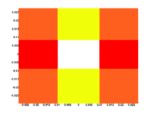
Figure 1: Uncorrelated case.

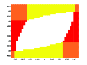
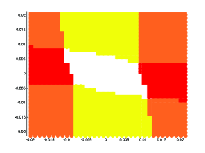
Figure 2: Negative correlation (left), positive correlation (right).

As expected and in line with the results of [33], the no-transaction region in the uncorrelated case is a rectangle. Then, under a possible correlation between the assets, the shape of the region is modified to a parallelogram, the direction of the deformation depending on the sign of the correlation.

In the next Figure 3, we keep the same transaction costs structure and we consider the higher correlations induced by the volatility matrices:

$$\sigma_{--}=\left(\begin{matrix}1&-0.25\\ -0.1&1\end{matrix}\right) \sigma_{++}=\left(\begin{matrix}1&0.25\\ 0.1&1\end{matrix}\right).$$ and

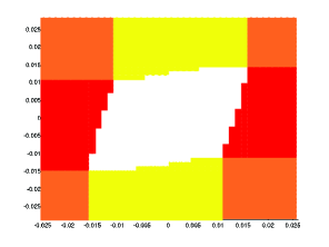
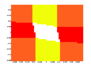
Figure 3: Higher correlations: negative (left) and positive (right).

By comparing them to the first figures, we observe that modifying the correlation induces a rotation of the no-transaction regions.

Our last Figure 4 for this section shows the impact of letting the transaction costs from one asset to the cash be higher than for the other asset. To isolate this effect we consider again the uncorrelated case $\sigma_{0}$, and choose $\lambda^{\prime}=\left(\begin{matrix}0&0.001&0.002\\ 0.001&0&\infty\\ 0.002&\infty&0\end{matrix}\right).$

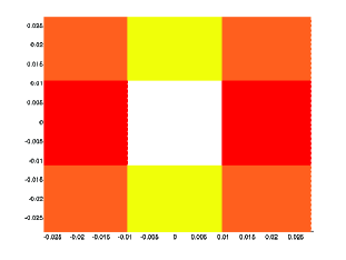
Figure 4: Different transaction costs.

As expected, we still observe a rectangle but with modified dimensions. More precisely, transactions between the first asset and the cash account occur more often since they are cheaper.

4.3.2 Possible transfers between all assets

In this section we allow for transactions between all assets, a feature which was not considered in any of the existing numerical approximations in the literature on the present problem. We start by fixing a symmetric transaction costs structure $\lambda_{0}$, and we illustrate the impact of correlation by considering the volatility matrices $\sigma_{0}$, $\sigma_{-}$ and $\sigma_{+}$.

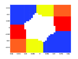
Figure 5: Uncorrelated case.

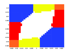
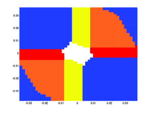
Figure 6: Negative correlation (left), positive correlation (right).

Our first observation is that transactions between the two assets do occur, and more importantly that as a consequence, the no transaction region seems to no longer be convex, an observation which, as far as we know, was not made before in the literature. Moreover, as in the previous section, the introduction of correlation induces a deformation of the no-transaction region. In order to insist on this loss of convexity, we also report the following figure obtained with the same parameters as the left side of Figure (5), but with more precise computations and without colors

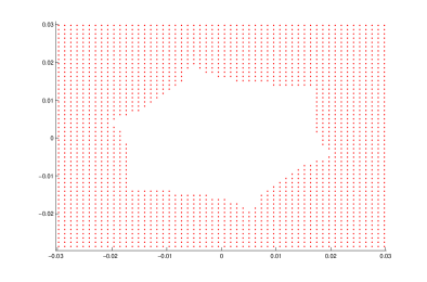
Figure 7: All transactions allowed.

Our last figure shows the impact of an asymmetric transaction costs structure. The volatility matrix is set to $\sigma_{0}$ and the transaction costs matrix to $\lambda^{\prime}$. As expected, there are almost no transactions between the cash account and asset $1$, since they are twice as expensive as the other ones. Surprisingly, we also observe the occurrence of small zones (in black and violet), where transactions are simultaneously performed between the assets and between the assets and the cash account.

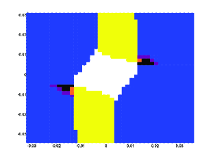
Figure 8: Asymmetric transaction costs.

5 Convergence

In the rest of the paper, we denote for any function $f(s,x,y)$:

$$\hat{f}(s,z,\xi):=f\big{(}s,z-{\bf y}(s,z)\cdot{\bf 1}_{d},\epsilon\xi+{\bf y}(s,z)\big{)}.$$

This section is dedicated to the proof of our main result, Theorem 3.3. Let:

$$u^{\epsilon}(s,x,y):=\bar{u}^{\epsilon}(s,x,y)-\epsilon^{2}w(s,z,\xi),\ s\in\mathbb{R}_{+}^{d},\ (x,y)\in K_{\epsilon}.$$

5.1 First estimates and properties

We start by obtaining several estimates of $u^{\epsilon}$. Set

$$\overline{\lambda}:=\underset{0\leq i,j\leq d}{\max}\lambda^{i,j},\ \underline{\lambda}:=\underset{0\leq i,j\leq d}{\min}\lambda^{i,j}.$$

We also recall that $L$ is the upper bound of the set $C$.

Lemma 5.1.

For $(\epsilon,s,x,y)\in(0,+\infty)\times(0,+\infty)^{d}\times K_{\epsilon}$, and $z:=x+y$, we have

$$u^{\epsilon}(s,x,y)\geq-\epsilon Lv_{z}(s,z)\left|y-{\bf y}(s,z)\right|.$$

Consequently, under Assumption 3.2, we have for all $(\epsilon,s,x,y)\in(0,+\infty)\times(0,+\infty)^{d}\times K_{\epsilon}$

$$0\leq u_{*}(s,x,y)\leq u^{*}(s,x,y)<+\infty.$$

Proof. Since $v^{\epsilon}(s,x,y)\leq v(s,z)$, it follows from the definition of $u^{\epsilon}$ that

$$u^{\epsilon}(s,x,y)\geq-\epsilon^{2}w(s,z,\xi).$$

Next, recall that $D\overline{w}$ takes values in the bounded set $C$. Since $w(.,0)=0$, this implies that $-w(s,z,\xi)\geq-L\left|\xi\right|v_{z}(s,z)$, and completes the proof. ∎

The next Lemma proves that the relaxed semi-limits are only functions of $(s,z)$.

Lemma 5.2.

Let Assumptions 3.1 and 3.2 hold. Then, $u^{*}$ and $u_{*}$ are only functions of $(s,z)$. Furthermore, we have

$$u_{*}(s,z) = \underset{(\epsilon,s^{\prime},z^{\prime})\rightarrow(0,s,z)}{\underline{\lim}}u^{\epsilon}\big{(}s^{\prime},z^{\prime}-{\bf y}(s^{\prime},z^{\prime})\cdot{\bf 1}_{d},{\bf y}(s^{\prime},z^{\prime})\big{)}$$

$$u^{*}(s,z) = \underset{(\epsilon,s^{\prime},z^{\prime})\rightarrow(0,s,z)}{\overline{\lim}}u^{\epsilon}\big{(}s^{\prime},z^{\prime}-{\bf y}(s^{\prime},z^{\prime})\cdot{\bf 1}_{d},{\bf y}(s^{\prime},z^{\prime})\big{)}.$$

Proof. We proceed in several steps. We assume throughout the proof that the parameter $\epsilon$ is less than one.

Step $1$: In view of the gradient constraints of the dynamic programming equation satisfied by $v^{\epsilon}$, we know that for all $1\leq i\leq d$, we have in the viscosity sense

$$\Lambda^{\epsilon}_{i,0}.(v^{\epsilon}_{x},v^{\epsilon}_{y})\geq 0,\ \Lambda^{\epsilon}_{0,i}.(v^{\epsilon}_{x},v^{\epsilon}_{y})\geq 0.$$ (5.1)

Now define

$$\widehat{v}^{\epsilon}(s,z,\xi):=v^{\epsilon}(s,z-\epsilon\xi\cdot{\bf 1}_{d}-{\bf y}(s,z)\cdot{\bf 1}_{d},\epsilon\xi+{\bf y}(s,z)).$$

We directly calculate that (5.1) implies for all $1\leq i\leq d$ in the viscosity sense

$$\epsilon^{4}\lambda^{i,0}\widehat{v}^{\epsilon}_{z}(s,z,\xi)-\epsilon^{3}\lambda^{i,0}{\bf y}_{z}(s,z).\widehat{v}^{\epsilon}_{\xi}(s,z,\xi)+(1+\epsilon^{3}\lambda^{i,0})\widehat{v}^{\epsilon}_{\xi^{i}}(s,z,\xi)\geq 0,$$ (5.2)

and

$$\epsilon^{4}\lambda^{0,i}\widehat{v}^{\epsilon}_{z}(s,z,\xi)-\epsilon^{3}\lambda^{0,i}{\bf y}_{z}(s,z).\widehat{v}^{\epsilon}_{\xi}(s,z,\xi)-\widehat{v}^{\epsilon}_{\xi^{i}}\geq 0.$$ (5.3)

Using the fact that all the ${\bf y}^{i}_{z}(s,z)$ are strictly positive (see Assumption 3.1), we can multiply (5.2) by ${\bf y}^{i}_{z}(s,z)$ and sum to obtain, once more in the viscosity sense

$$\left(1-\epsilon^{3}\sum_{i=1}^{d}\frac{{\bf y}^{i}_{z}(s,z)\lambda^{i,0}}{1+\epsilon^{3}\lambda^{i,0}}\right){\bf y}_{z}(s,z).\widehat{v}^{\epsilon}_{\xi}(s,z,\xi)\geq-\epsilon^{4}\sum_{i=1}^{d}\frac{\lambda^{i,0}}{1+\epsilon^{3}\lambda^{i,0}}\widehat{v}^{\epsilon}_{z}(s,z,\xi).$$ (5.4)

Now, we have by Assumption 3.1

$$1-\epsilon^{3}\sum_{i=1}^{d}\frac{{\bf y}^{i}_{z}(s,z)\lambda^{i,0}}{1+\epsilon^{3}\lambda^{i,0}}=1-\sum_{i=1}^{d}{\bf y}_{z}^{i}(s,z)+\sum_{i=1}^{d}\frac{{\bf y}^{i}_{z}(s,z)}{1+\epsilon^{3}\lambda^{i,0}}\geq 0.$$

Using this inequality in (5.4) yields, in the viscosity sense

$${\bf y}_{z}(s,z).\widehat{v}^{\epsilon}_{\xi}(s,z,\xi)\geq-\frac{\sum_{i=1}^{d}\frac{\lambda^{i,0}}{1+\epsilon^{3}\lambda^{i,0}}}{1-\epsilon^{3}\sum_{i=1}^{d}\frac{{\bf y}^{i}_{z}(s,z)\lambda^{i,0}}{1+\epsilon^{3}\lambda^{i,0}}}\epsilon^{4}\widehat{v}^{\epsilon}_{z}(s,z,\xi).$$ (5.5)

Plugging this estimate in (5.2) and (5.3), we obtain in the viscosity sense

$$\widehat{v}^{\epsilon}_{\xi^{i}}(s,z,\xi)\leq\lambda^{0,i}\epsilon^{4}\left(1+\frac{\sum_{i=1}^{d}\frac{\lambda^{i,0}}{1+\epsilon^{3}\lambda^{i,0}}}{1-\epsilon^{3}\sum_{i=1}^{d}\frac{{\bf y}^{i}_{z}(s,z)\lambda^{i,0}}{1+\epsilon^{3}\lambda^{i,0}}}\right)\widehat{v}^{\epsilon}_{z}(s,z,\xi)\leq\epsilon^{4}\overline{\lambda}\left(1+\frac{\overline{\lambda}d}{c_{0}}\right)\widehat{v}^{\epsilon}_{z}(s,z,\xi),$$

and

$$\widehat{v}^{\epsilon}_{\xi^{i}}(s,z,\xi)\geq-2\epsilon^{4}\underline{\lambda}\widehat{v}^{\epsilon}_{z}(s,z,\xi).$$

By the concavity of $v^{\epsilon}$, its gradient exists almost everywhere. Moreover, since we assumed that ${\bf y}$ is smooth, this implies that $\widehat{v}^{\epsilon}_{z}$ also exists almost everywhere. Hence, we conclude from the above estimates that

$$\left|\widehat{v}^{\epsilon}_{\xi}\right|\leq A\epsilon^{4}\widehat{v}^{\epsilon}_{z}, A:=\sqrt{d}\max\Big{\{}\overline{\lambda}\Big{(}1+\frac{\overline{\lambda}^{2}d}{c_{0}}\Big{)},2\underline{\lambda}\Big{\}}.$$ where (5.6)

Step $2$: We now prove an estimate for $\widehat{v}^{\epsilon}_{z}$. By definition and from Assumption 3.1,

$$\widehat{v}^{\epsilon}_{z}(s,z,\xi) =\partial_{z}v^{\epsilon}\left(s,z-\epsilon\xi\cdot{\bf 1}_{d}-{\bf y}(s,z)\cdot{\bf 1}_{d},\epsilon\xi+{\bf y}(s,z)\right)$$

$$=\left(1-{\bf y}_{z}(s,z)\cdot{\bf 1}_{d}\right)v^{\epsilon}_{x}(s,x,y)+{\bf y}_{z}(s,z).v^{\epsilon}_{y}(s,x,y)$$

$$\leq v^{\epsilon}_{x}(s,x,y)+v_{y}^{\epsilon}(s,x,y)\cdot{\bf 1}_{d}.$$ (5.7)

Therefore, we can focus on obtaining estimates on $v^{\epsilon}_{x}$ and $v^{\epsilon}_{y}$. First, by concavity of $v^{\epsilon}$ in $x$ and of $v$ in $z$, we have

$$v^{\epsilon}_{x}(s,x,y) \leq\frac{v^{\epsilon}(s,x,y)-v^{\epsilon}(s,x-\epsilon,y)}{\epsilon}$$

$$\leq\frac{v(s,z)-v(s,z-\epsilon)}{\epsilon}+\frac{v(s,z-\epsilon)-v^{\epsilon}(s,x-\epsilon,y)}{\epsilon}$$

$$\leq v_{z}(s,z-\epsilon)+\frac{v(s,z-\epsilon)-v^{\epsilon}(s,x-\epsilon,y)}{\epsilon}.$$

Now, using the definition of $u^{\epsilon}$, we obtain

$$v^{\epsilon}_{x}(s,x,y)\leq v_{z}(s,z-\epsilon)+\epsilon\left(u^{\epsilon}(s,x-\epsilon,y)+\epsilon^{2}w(s,z-\epsilon,\xi_{\epsilon})\right),$$

where

$$\xi_{\epsilon}:=\frac{y-{\bf y}(s,z-\epsilon)}{\epsilon}=\xi+\frac{{\bf y}(s,z)-{\bf y}(s,z-\epsilon)}{\epsilon}.$$

From the estimates on $w$ in Theorem 3.1 and Assumption 3.4, we have

$$\left|w(s,z-\epsilon,\xi_{\epsilon})\right|\leq Lv_{z}(s,z)(1+\left|\xi_{\epsilon}\right|)\leq Lv_{z}(s,z)\left(1+\left|\xi\right|+\frac{\left|{\bf y}(s,z)-{\bf y}(s,z-\epsilon)\right|}{\epsilon}\right),$$

and therefore

$$v^{\epsilon}_{x}(s,x,y)\leq v_{z}(s,z-\epsilon)+\epsilon u^{\epsilon}(s,x-\epsilon,y)+\epsilon^{3}Lv_{z}(s,z)\left(1+\left|\xi\right|+\frac{\left|{\bf y}(s,z)-{\bf y}(s,z-\epsilon)\right|}{\epsilon}\right).$$

As for $v^{\epsilon}_{y}$, we use again the concavity of $v^{\epsilon}$ and $v$ in $y$ and $z$, respectively,

$$v^{\epsilon}_{y^{i}}(s,x,y) \leq\frac{v^{\epsilon}(s,x,y)-v^{\epsilon}(s,x,y-\epsilon e_{i})}{\epsilon}$$

$$\leq\frac{v(s,z)-v(s,z-\epsilon)}{\epsilon}+\frac{v(s,z-\epsilon)-v^{\epsilon}(s,x,y-\epsilon e_{i})}{\epsilon}$$

$$\leq v_{z}(s,z-\epsilon)+\frac{v(s,z-\epsilon)-v^{\epsilon}(s,x,y-\epsilon e_{i})}{\epsilon},\leavevmode\nobreak\ \leavevmode\nobreak\ 0\leq i\leq d.$$

Similarly as above, this yields

$$v^{\epsilon}_{y^{i}}(s,x,y) \leq v_{z}(s,z-\epsilon)+\epsilon u^{\epsilon}(s,x,y-\epsilon e_{i})$$

$$+\epsilon^{3}Lv_{z}(s,z)\left(1+\left|\xi\right|+\frac{\left|-\epsilon e_{i}+{\bf y}(s,z)-{\bf y}(s,z-\epsilon)\right|}{\epsilon}\right).$$

Plugging the above estimates in (5.1), we get

$$\widehat{v}^{\epsilon}_{z}(s,z,\epsilon)\leq (1+d)v_{z}(s,z-\epsilon)+\epsilon\left(u^{\epsilon}(s,x-\epsilon,y)+\sum_{i=1}^{d}u^{\epsilon}(s,x,y-\epsilon e_{i})\right)$$ (5.8)

$$+\epsilon^{3}Lv_{z}(s,z)\left(d+(1+d)\left(1+\left|\xi\right|+\frac{\left|{\bf y}(s,z)-{\bf y}(s,z-\epsilon)\right|}{\epsilon}\right)\right)=:\gamma^{\epsilon}(s,z,\xi).$$

Step $3$ Recall that $\widehat{v}^{\epsilon}_{z}$ exists almost everywhere, and thus by definition of $u^{\epsilon}$, this also holds for $\widehat{u}^{\epsilon}_{z}$ and $\widehat{u}^{\epsilon}_{\xi}$. Now, using (5.6), (5.8) together with Assumption 3.1 and our estimates on $w$, we obtain for some constant $C>0$

$$\left|\widehat{u}^{\epsilon}_{\xi}(s,z,\xi)\right|\leq\epsilon^{2}C\left(v_{z}(s,z)+\widehat{v}^{\epsilon}_{z}(s,z,\xi)\right)\leq\epsilon^{2}C\left(v_{z}(s,z)+\gamma^{\epsilon}_{z}(s,z,\xi)\right).$$

With this estimate, we can conclude the proof exactly as in the proof of Lemma $6.2$ in [44]. ∎

5.2 Remainder estimate

In this section, we isolate an estimate which will be needed at various occasions in the subsequent proofs. The following calculation extends the estimate of Section 4.2 in [44]. For any function

$$\Psi^{\epsilon}(s,x,y):=v(s,z)-\epsilon^{2}\phi(s,z)-\epsilon^{4}\varpi(s,z,\xi),$$

with smooth $\phi$ and $\upsilon$ such that $\upsilon$ also verifies the estimates (3.5), we have

$$\mathcal{I}(\Psi^{\epsilon})(s,x,y): =\left(\beta\Psi^{\epsilon}-\mathcal{L}\Psi^{\epsilon}-\widetilde{U}(\Psi^{\epsilon}_{x})\right)(s,x,y)$$

$$=\epsilon^{2}\left[-\frac{1}{2}\left|\sigma(s)\xi\right|v_{zz}+\frac{1}{2}{\rm Tr}\left[\alpha\alpha^{T}(s,z)\varpi_{\xi\xi}(s,z,\xi)\right]-\mathcal{A}\phi(s,z)+\mathcal{R}^{\epsilon}(s,z,\xi)\right].$$

Similarly as in [44], direct but tedious calculations provides the following estimate:

$$\left|\mathcal{R}^{\epsilon}(s,x,y)\right|\leq \epsilon\Big{(}\left|\mu-r\cdot{\bf 1}_{d}\right|\left|\xi\right|\left|\phi_{z}\right|+\frac{\left|\sigma\right|^{2}}{2}\left(2\left|{\bf y}\right|\left|\xi\right|+\epsilon\xi^{2}\right)\left|\phi_{zz}\right|+\left|\sigma\right|^{2}\left|\xi\right|\left|D_{sz}\phi\right|\Big{)}(s,z)$$

$$+\epsilon C(s,z)\left(1+\epsilon\left|\xi\right|+\epsilon^{2}\left|\xi\right|^{2}+\epsilon^{3}\left|\xi\right|^{3}\right)$$

$$+\epsilon^{-2}\left|\widetilde{U}(\Psi^{\epsilon}_{x})-\widetilde{U}(v_{z})-(\Psi^{\epsilon}_{x}-v_{z})\widetilde{U}^{{}^{\prime}}(v_{z})\right|,$$

for some continuous function $C(s,z)$. Now using the fact $\widetilde{U}$ is $C^{1}$ and convex and the estimates assumed for $\upsilon$, we obtain

$$\left|\mathcal{R}^{\epsilon}(s,x,y)\right|\leq \epsilon\Big{(}\left|\mu-r\cdot{\bf 1}_{d}\right|\left|\xi\right|\left|\phi_{z}\right|+\frac{\left|\sigma\right|^{2}}{2}\left(2\left|{\bf y}\right|\left|\xi\right|+\epsilon\xi^{2}\right)\left|\phi_{zz}\right|+\left|\sigma\right|^{2}\left|\xi\right|\left|D_{sz}\phi\right|\Big{)}(s,z)$$

$$+\epsilon C(s,z)\left(1+\epsilon\left|\xi\right|+\epsilon^{2}\left|\xi\right|^{2}+\epsilon^{3}\left|\xi\right|^{3}\right)$$

$$+\epsilon^{2}\left(\left|\phi_{z}\right|+\epsilon C(s,z)(1+\epsilon\left|\xi\right|)\right)^{2}\widetilde{U}^{{}^{\prime\prime}}\left(v_{z}+\epsilon^{2}\left|\phi_{z}\right|+\epsilon^{3}C(s,z)(1+\epsilon\left|\xi\right|)\right).$$

5.3 Viscosity subsolution property

In this Section, we prove

Proposition 5.1.

Under Assumptions 3.1, 3.2 and 3.4, the function $u^{*}$ is a viscosity subsolution of the second corrector equation.

Proof. Let $(s_{0},z_{0},\phi)\in(0,+\infty)^{d}\times(0,+\infty)\times C^{2}\left((0,+\infty)^{d}\times(0,+\infty)\right)$ be such that

$$(u^{*}-\phi)(s_{0},z_{0})>(u^{*}-\phi)(s,z),\text{ for all $(s,z)\in(0,+\infty)^{d}\times(0,+\infty)\backslash\left\{(s_{0},z_{0})\right\}$}.$$ (5.9)

By definition of viscosity subsolutions, we need to show that

$$\mathcal{A}\phi(s_{0},z_{0})-a(s_{0},z_{0})\leq 0.$$

We will proceed in several steps.

Step $1$: First of all, we know from Lemma 5.2 that there exists a sequence $(s^{\epsilon},z^{\epsilon})$ which realizes the $\limsup$ for $\widehat{u}^{\epsilon}$, that is to say

$$(s^{\epsilon},z^{\epsilon})\underset{\epsilon\downarrow 0}{\longrightarrow}(s_{0},z_{0})\text{ and }\widehat{u}^{\epsilon}(s^{\epsilon},z^{\epsilon},0)\underset{\epsilon\downarrow 0}{\longrightarrow}u^{*}(s_{0},z_{0}).$$

It follows then easily that $l^{\epsilon}_{*}:=\widehat{u}^{\epsilon}(s^{\epsilon},z^{\epsilon},0)-\phi(s^{\epsilon},z^{\epsilon})\underset{\epsilon\downarrow 0}{\longrightarrow}0,$ and

$$(x^{\epsilon},y^{\epsilon})=\left(z^{\epsilon}-{\bf y}(s^{\epsilon},z^{\epsilon})\cdot{\bf 1}_{d},{\bf y}(s^{\epsilon},z^{\epsilon})\right)\underset{\epsilon\downarrow 0}{\longrightarrow}(x_{0},y_{0}):=\left(z_{0}-{\bf y}(s_{0},z_{0})\cdot{\bf 1}_{d},{\bf y}(s_{0},z_{0})\right).$$

Now recall from Assumption 3.2 that $u^{\epsilon}$ is locally bounded from above. This implies the existence of $r_{0}:=r_{0}(s_{0},x_{0},y_{0})>0$ and $\epsilon_{0}:=\epsilon_{0}(s_{0},x_{0},y_{0})>0$ verifying

$$b_{*}:=\sup\left\{u^{\epsilon}(s,x,y),\ (s,x,y)\in B_{0},\ \epsilon\in(0,\epsilon_{0}]\right\}<+\infty,$$ (5.10)

where $B_{0}:=B_{r_{0}}(s_{0},x_{0},y_{0})$ is the open ball with radius $r_{0}$ and center $(s_{0},x_{0},y_{0})$. Moreover, notice that we can always decrease $r_{0}$ so that $r_{0}\leq z_{0}/2$, which then implies that $B_{0}$ does not cross the line $z=0$. Now for any $(\epsilon,\delta)\in(0,1]^{2}$, we define $\Psi^{\epsilon,\delta}$ and the corresponding $\hat{\Psi}^{\epsilon,\delta}$ by

$$\widehat{\Psi}^{\epsilon,\delta}(s,z,\xi):=v(s,z)-\epsilon^{2}\left(l_{*}^{\epsilon}+\phi(s,z)+\widehat{\Phi}^{\epsilon}(s,z,\xi)\right)-\epsilon^{4}(1+\delta)w(s,z,\xi),$$

where the function $\hat{\Phi}^{\epsilon}$ and the corresponding $\Phi^{\epsilon}$ are given by:

$$\hat{\Phi}^{\epsilon}(s,x,y):=c_{0}\Big{(}(s-s^{\epsilon})^{4}+(z-z^{\epsilon})^{4}+\epsilon^{4}w^{4}(s,z,\xi)\Big{)},$$

and $c_{0}>0$ is a constant chosen large enough in order to have for $\epsilon$ small enough

$$\Phi^{\epsilon}\leq 1+b_{*}-\phi,\text{ on }B_{0}\backslash B_{1},\text{ where }B_{1}:=B_{\frac{r_{0}}{2}}(s_{0},x_{0},y_{0}).$$ (5.11)

We emphasize that the constant $c_{0}$ may depend on $(\phi,s_{0},x_{0},y_{0},\delta)$ but not on $\epsilon$, and that a priori the function $\widehat{\Psi}^{\epsilon,\delta}$ is not $C^{2}$ in $\xi$, because the function $w$ is only in $C^{1,1}$. This is a major difference with the one-dimension case treated in [44].

Step $2$: We now prove that for all sufficiently small $\epsilon$ and $\delta$, the difference $(v^{\epsilon}-\Psi^{\epsilon,\delta})$ has a local minimizer in $B_{0}$. First, notice that this is equivalent to showing that the following quantity has a local minimizer in $B_{0}$

$$I^{\epsilon,\delta}(s,x,y): =\frac{v^{\epsilon}(s,x,y)-\Psi^{\epsilon,\delta}(s,x,y)}{\epsilon^{2}}$$

$$=-u^{\epsilon}(s,x,y)+l_{*}^{\epsilon}+\phi(s,z)+\phi^{\epsilon}(s,x,y)+\epsilon^{2}\delta w(s,z,\xi).$$

By (5.11) and the fact that $w\geq 0$, we have for any $(s,x,y)\in\partial B_{0}$

$$I^{\epsilon,\delta}(s,x,y)\geq-u^{\epsilon}(s,x,y)+l_{*}^{\epsilon}+1+b_{*}+\epsilon^{2}\delta w(s,z,\xi)\geq 1+l_{*}^{\epsilon}>0,$$

for $\epsilon$ small enough. Moreover, since $I^{\epsilon,\delta}(s^{\epsilon},x^{\epsilon},y^{\epsilon})=0$, this implies that $I^{\epsilon,\delta}$ has a local minimizer $(\tilde{s}^{\epsilon},\tilde{x}^{\epsilon},\tilde{y}^{\epsilon})$ in $B_{0}$, and we introduce the corresponding

$$\tilde{z}^{\epsilon}:=\tilde{x}^{\epsilon}+\tilde{y}^{\epsilon}\cdot{\bf 1}_{d},\text{ and }\tilde{\xi}^{\epsilon}:=\frac{\tilde{y}^{\epsilon}-{\bf y}(\tilde{s}^{\epsilon},\tilde{z}^{\epsilon})}{\epsilon}.$$

We then have

$$\underset{(s,z,\xi)}{\min}(\widehat{v}^{\epsilon}-\widehat{\Psi}^{\epsilon,\delta})(s,z,\xi)=(\widehat{v}^{\epsilon}-\Psi^{\epsilon,\delta})(\tilde{s}^{\epsilon},\tilde{z}^{\epsilon},\tilde{\xi}^{\epsilon})\leq 0,\ \left|\tilde{s}^{\epsilon}-s_{0}\right|+\left|\tilde{z}^{\epsilon}-z_{0}\right|\leq r_{0},\ \left|\tilde{\xi}^{\epsilon}\right|\leq\frac{r_{1}}{\epsilon},$$

for some constant $r_{1}$. We now use the viscosity supersolution property of $v^{\epsilon}$. Since $\Psi^{\epsilon,\delta}$ is $C^{1}$, we obtain from the first order operator in the dynamic programming equation that:

$$\Lambda^{\epsilon}_{i,j}\cdot\big{(}\Psi_{x}^{\epsilon,\delta},\Psi_{y}^{\epsilon,\delta}\big{)}(\tilde{s}^{\epsilon},\tilde{x}^{\epsilon},\tilde{y}^{\epsilon})\geq 0 0\leq i,j\leq d.$$ for all (5.12)

Step $3$: In this step, we show that for $\epsilon$ small enough, we have

$$\tilde{\rho}^{\epsilon}\;:=\;\frac{\tilde{\xi}^{\epsilon}}{\eta(\tilde{s}^{\epsilon},\tilde{z}^{\epsilon})}\;\in\;\mathcal{O}_{0}(\tilde{s}^{\epsilon},\tilde{z}^{\epsilon}).$$ (5.13)

where $\mathcal{O}_{0}(s,z)$ is the open set of Proposition 3.2. We argue by contradiction assuming that there exists some sequence $\epsilon_{n}\longrightarrow 0$ such that $\tilde{\rho}^{\epsilon_{n}}\not\in\mathcal{O}_{0}(\tilde{s}^{\epsilon_{n}},\tilde{z}^{\epsilon_{n}})$. This implies that

$$-\lambda^{i_{0}^{n},j_{0}^{n}}+\big{(}\partial_{i_{0}^{n}}\overline{w}-\partial_{j_{0}^{n}}\overline{w}\big{)}(\tilde{s}^{\epsilon_{n}},\tilde{z}^{\epsilon_{n}},\tilde{\rho}^{\epsilon_{n}})=0 (i_{0}^{n},j_{0}^{n}).$$ for some (5.14)

By the gradient constraint (5.12), and the boundedness of $\big{(}\tilde{s}^{\epsilon_{n}},\tilde{z}^{\epsilon_{n}},\epsilon_{n}\tilde{\xi}^{\epsilon_{n}}\big{)}_{n}$, we directly compute that:

$$-4C\epsilon_{n}^{2}(\epsilon_{n}w)^{3}(\tilde{s}^{\epsilon_{n}},\tilde{z}^{\epsilon_{n}},\tilde{\xi}^{\epsilon_{n}})\left(w_{\xi^{i_{0}^{n}}}-w_{\xi^{j_{0}^{n}}}\right)(\tilde{s}^{\epsilon_{n}},\tilde{z}^{\epsilon_{n}},\tilde{\xi}^{\epsilon_{n}})$$

$$\hskip 8.99994pt+\epsilon_{n}^{3}v_{z}(\tilde{s}^{\epsilon_{n}},\tilde{z}^{\epsilon_{n}})\left[\lambda^{i_{0}^{n},j_{0}^{n}}-(1+\delta)(\partial_{i_{0}^{n}}\overline{w}-\partial_{j_{0}^{n}}\overline{w})(\tilde{s}^{\epsilon_{n}},\tilde{z}^{\epsilon_{n}},\tilde{\rho}^{\epsilon_{n}})\right]+\circ(\epsilon_{n}^{3})\geq 0.$$ (5.15)

Using (5.14) and the non-negativity of $w$, this implies

$$0 \leq -4c_{0}\lambda^{i_{0}^{n},j_{0}^{n}}\epsilon_{n}^{2}(\epsilon_{n}w)^{3}(\tilde{s}^{\epsilon_{n}},\tilde{z}^{\epsilon_{n}},\tilde{\xi}^{\epsilon_{n}})-\delta\lambda^{i_{0}^{n},j_{0}^{n}}\epsilon_{n}^{3}v_{z}(\tilde{s}^{\epsilon_{n}},\tilde{z}^{\epsilon_{n}})+\circ(\epsilon_{n}^{3})$$

$$\leq -\delta\lambda^{i_{0}^{n},j_{0}^{n}}\epsilon_{n}^{3}v_{z}(\tilde{s}^{\epsilon_{n}},\tilde{z}^{\epsilon_{n}})+\circ(\epsilon_{n}^{3})\geq 0,$$

which leads to a contradiction when $n$ goes to $+\infty$.

Step $4$: From (5.13) and Proposition 3.2, we deduce that in our domain of interest, the function $\Psi^{\epsilon,\delta}$ is actually smooth, and is therefore a legitimate test function for the second order operator of the dynamic programming equation. We then obtain from the supersolution property of $v^{\epsilon}$ that

$$\left(\beta v^{\epsilon}-\mathcal{L}\Psi^{\epsilon,\delta}-\widetilde{U}(\Psi_{x}^{\epsilon,\delta})\right)(\tilde{s}^{\epsilon},\tilde{x}^{\epsilon},\tilde{y}^{\epsilon})\geq 0.$$ (5.16)

Moreover, by Step $3$ and the continuity of $(s,z)\longmapsto\mathcal{O}(s,z)$ in Assumption 3.4, the sequence $(\tilde{\xi}^{\epsilon})_{\epsilon}$ is bounded. By classical results in the theory of viscosity solutions, there exists a sequence $\epsilon_{n}\rightarrow 0$ and some $\tilde{\xi}$ such that

$$(s_{n},z_{n},\xi_{n}):=(\tilde{s}^{\epsilon_{n}},\tilde{z}^{\epsilon_{n}},\tilde{\xi}^{\epsilon_{n}})\longrightarrow(s_{0},z_{0},\tilde{\xi}).$$

Now recall that the function $w$ is smooth in this case and that the function $\Psi^{\epsilon,\delta}$ has exactly the form given in Section 5.2. By the remainder estimate in (5.16), we obtain

$$\frac{1}{2}\eta(s_{n},z_{n})\left|\sigma(s_{n})\xi_{n}\right|^{2}+\frac{1}{2}(1+\delta){\rm Tr}\left[\alpha\alpha^{T}(s_{n},z_{n})w_{\xi\xi}(s_{n},z_{n},\xi_{n})\right]-\mathcal{A}\phi(s_{n},z_{n})+\mathcal{R}^{\epsilon}(s,z,\xi)\geq 0.$$

We still have no guarantee that $w$ is $C^{2}$ at $\widehat{\xi}$. Therefore, we carefully estimate the term involving $w_{\xi\xi}$. Indeed, the equation satisfied by $w$ yields

$$a(s_{n},z_{n})-\mathcal{A}\phi(s_{n},z_{n})+\delta\left(a(s_{n},z_{n})-\frac{1}{2}\eta(s_{n},z_{n})\left|\sigma(s_{n})\xi_{n}\right|^{2}\right)+\mathcal{R}^{\epsilon}(s,z,\xi)\geq 0.$$ (5.17)

Notice that the estimate on the remainder of Section 5.2 still hold true if terms involving $w_{\xi\xi}$ are replaced by means of the first corrector equation. Since the map $(s,z)\longmapsto a(s,z)$ is continuous, by Assumption 3.4, and all derivatives of $\Phi^{\epsilon}$ vanish at the origin, we may send $\epsilon$ to $0$ in (5.17) and obtain

$$a(s_{0},z_{0})-\mathcal{A}\phi(s_{0},z_{0})+\delta\left(a(s_{0},z_{0})-\frac{1}{2}\eta(s_{0},z_{0})|\sigma(s_{0})\tilde{\xi}|^{2}\right)\geq 0.$$ (5.18)

Since $\tilde{\xi}$ is bounded uniformly in $\delta$, we let $\delta$ go to zero in (5.18) to obtain the desired result. ∎

5.4 Viscosity supersolution property

In this section we will prove the following result.

Proposition 5.2.

Under Assumptions 3.1, 3.2 and 3.4, $u_{*}$ is a viscosity supersolution of the second corrector equation.

To prove this result, we start by two useful lemmas. For the first one, we recall that in the proof of the viscosity subsolution property in the previous section, we mentioned that the function $w$ is not $C^{2}$ in the whole space. We overcome this difficulty by using the fact that we only needed $w$ on a subset of $\mathbb{R}^{d}$ where it is actually smooth. However, in the proof of the viscosity supersolution property, we need $w$ to be defined on the whole space. Therefore, we mollify it and the following Lemma gives some useful properties satisfied by this mollified version of $w$.

Let $k:\mathbb{R}^{d}\rightarrow\mathbb{R}$ be a positive, even (i.e. $k(-x)=k(x)$ for all $x\in\mathbb{R}^{d}$), $C^{\infty}$ function with support in the closed unit ball of $\mathbb{R}^{d}$ and unit total mass. For all $m>0$, we define

$$k^{m}(x):=\frac{1}{m^{d}}k\Big{(}\frac{\xi}{m}\Big{)} w^{m}(s,z,\xi):=\int_{\mathbb{R}^{d}}k^{m}(\zeta)w(\xi-\zeta)d\zeta-\int_{\mathbb{R}^{d}}k^{m}(\zeta)w(-\zeta)d\zeta.$$ and

Lemma 5.3.

Let Assumption 3.4 hold. For any $m>0$, the function $w^{m}$ satisfies:

$\rm{(i)}$ $w^{m}$ is $C^{2}$, convex in $\xi$, and we have for all $0\leq i,j\leq d$

$$w^{m}_{\xi_{i}}(s,z,\xi)=\int_{\mathbb{R}^{d}}k^{m}(\zeta)w_{\xi_{i}}(s,z,\xi-\zeta)d\zeta,\text{ }w^{m}_{\xi_{i}\xi_{j}}(s,z,\xi)=\int_{\mathbb{R}^{d}}k^{m}(\zeta)w_{\xi_{i}\xi_{j}}(s,z,\xi-\zeta)d\zeta.$$

Moreover, $0\leq w^{m}(s,z,\xi)\leq Lv_{z}(s,z)\left|\xi\right|.$

$\rm{(ii)}$ $w^{m}$ is smooth in $(s,z)$, and satisfies the following estimates, uniformly in $m$,

$$\left(\left|w^{m}\right|+\left|w^{m}_{s}\right|+\left|w^{m}_{ss}\right|+\left|w^{m}_{z}\right|+\left|w^{m}_{sz}\right|+\left|w^{m}_{zz}\right|\right)(s,z,\xi)\leq C(s,z)\left(1+\left|\xi\right|\right)$$

$$\left(\left|w^{m}_{\xi}\right|+\left|w^{m}_{s\xi}\right|+\left|w^{m}_{z\xi}\right|\right)(s,z,\xi)\leq C(s,z)$$

$$\left|w^{m}_{\xi\xi}(s,z,\xi)\right|\leq C(s,z)1_{\xi\in B(s,z)},$$ (5.19)

where $C(s,z)$ is a continuous function depending on the Merton value function and its derivatives, and $B(s,z)$ is small ball with continuous radius and center in $(s,z)$.

$\rm{(iii)}$ For every $0\leq i,j\leq d$ and every $(s,z,\xi)$

$$-\lambda^{i,j}v_{z}(s,z)+w^{m}_{\xi_{i}}(s,z,\xi)-w^{m}_{\xi_{j}}(s,z,\xi)\leq 0.$$

$\rm{(iv)}$ For every $(s,z,\xi)$, we have

$$\frac{1}{2}v_{zz}(s,z)\int_{\mathbb{R}^{d}}k^{m}(x)\left|\sigma(s)(\xi-\zeta)\right|^{2}d\zeta-\frac{1}{2}{\rm Tr}\left[\alpha\alpha^{T}(s,z)w^{m}_{\xi\xi}(s,z,\xi)\right]+a(s,z)\leq 0.$$

Proof. $\rm{(i)}$ The fact that $w^{m}$ is $C^{2}$ in $\xi$ is a classical result. Moreover, we have by definition $w^{m}(s,z,0)=0$ and by convexity of $w$, we have $w^{m}\geq w\geq 0$. The equalities for the derivatives of $w^{m}$ follow from the fact that $w$ is $C^{1}$ in $\xi$ and $C^{2}$ almost everywhere. Finally, $w^{m}$ inherits clearly the convexity and Lipschitz property of $w$.

$\rm{(ii)}$ is clear by linearity of the convolution and Assumption 3.4. $\rm{(iii)}$ is again a consequence of the linearity of the convolution and the gradient constraints satisfied by $w$. Finally $\rm{(iv)}$ follows from the linearity of the convolution, the second corrector equation satisfied by $w$ and the formula for $w^{m}_{\xi\xi}$ given in $\rm{(i)}$. ∎

We next constructs a useful function which plays a major role in our subsequent proof.

Lemma 5.4.

For any $\delta\in(0,1)$, there exists $a^{\delta}>1$ and a function $h^{\delta}:\mathbb{R}^{d}\rightarrow[0,1]$ such that $h^{\delta}$ is $C^{\infty}$, $h^{\delta}=1$ on $\mathcal{B}_{1}(0)$ and $h^{\delta}=0$ on $B_{a^{\delta}}(0)^{c}$. Moreover, for any $1\leq i\leq d$ and for any $\xi\in\mathbb{R}^{d}$

$$\left|h^{\delta}_{\xi_{i}}(\xi)\right|\leq\frac{\delta}{2L\overline{\lambda}}{\bf 1}_{B_{a^{\delta}}(0)}(\xi),\text{ and }\left|\xi\right||h^{\delta}_{\xi\xi}|\leq C^{*},$$

for some constant $C^{*}$ independent of $\delta$.

Proof. Let $\phi$ be an even $C^{\infty}$ function on $\mathbb{R}_{+}$, whose support is in $(-1,1)$, such that $0\leq\phi\leq 1$ and $\int_{-1}^{1}\phi(t)dt=1$. For some $\alpha>0$ to be specified later, we define the following function $\tilde{h}^{\alpha}:\mathbb{R}_{+}\longrightarrow[0,1]$:

$$\tilde{h}_{\alpha}(x):=\int_{-1}^{1}H^{\alpha}(x-t)\phi(t)dt,\text{ where }H^{\alpha}(x):={\bf 1}_{\{x\leq 2\}}+\Big{(}1-\alpha\ln\Big{(}\frac{x}{2}\Big{)}\Big{)}{\bf 1}_{\{2<x\leq 2e^{1/\alpha}\}}.$$

Clearly, $\tilde{h}_{\alpha}$ is $C^{\infty}$, $\tilde{h}_{\alpha}=1$ on $[0,1]$ and to $\tilde{h}_{\alpha}=0$ for $[1+2e^{1/\alpha},\infty)$. Moreover, $\tilde{h}_{\alpha}$ is decreasing and its derivative clearly verifies for every $x\in\mathbb{R}$

$$0\geq\tilde{h}_{\alpha}^{\prime}(x)\geq-\frac{\alpha}{2}.$$ (5.20)

We claim that

$$\left|x\tilde{h}_{\alpha}^{\prime\prime}(x)\right|\leq\frac{3\alpha}{4} x\in\mathbb{R}.$$ for all (5.21)

Indeed, this inequality is obvious on $(-\infty,1]$, and we compute for $x\geq 1$, that

$$0\leq x\tilde{h}_{\alpha}^{\prime\prime}(x)=\int_{-1}^{1}\frac{\alpha x}{(x-t)^{2}}{\bf 1}_{\{2<x-t\leq 2e^{1/\alpha}\}}\phi(t)dt\leq\int_{-1}^{1}\alpha\frac{3}{4}\phi(t)dt=\frac{3\alpha}{4}.$$

We now introduce the function:

$$h^{\delta}(\xi):=\tilde{h}_{\tilde{\delta}}\left(\left|\xi\right|\right),\leavevmode\nobreak\ \leavevmode\nobreak\ \tilde{\delta}:=\frac{\delta}{L\overline{\lambda}}\leavevmode\nobreak\ \leavevmode\nobreak\ \xi\in\mathbb{R}^{d}.$$

Clearly $h^{\delta}$ is $C^{\infty}$, takes values in $[0,1]$, $h^{\delta}=1$ on $B_{0}(1)$, and $h^{\delta}=0$ on $B_{1+2e^{L/\delta}}(0)^{c}$. In particular, this provides the existence of $a^{\delta}\in[1,1+2e^{\frac{L}{\delta}}]$. Also

$$h^{\delta}_{\xi_{i}}(\xi)=\tilde{h}_{\tilde{\delta}}^{\prime}(\left|\xi\right|)\frac{\xi_{i}}{\left|\xi\right|}.$$

Thus, by (5.20) and the fact that $\tilde{h}_{\tilde{\delta}}$ and all its derivatives vanish on $(a^{\delta},\infty)$:

$$\left|h^{\delta}_{\xi_{i}}(\xi)\right|\leq\frac{\delta}{2L\overline{\lambda}}{\bf 1}_{B_{a^{\delta}}(0)}(x).$$

Similarly, we have

$$\left|\xi\right|h^{\delta}_{\xi\xi}(\xi)=\Big{(}\left|\xi\right|\tilde{h}_{\tilde{\delta}}^{\prime\prime}(\left|\xi\right|)-\frac{1}{2}\tilde{h}_{\tilde{\delta}}^{\prime}(\left|\xi\right|)\Big{)}\frac{\xi\xi^{T}}{\left|\xi\right|^{2}}+\tilde{h}_{\tilde{\delta}}^{\prime}(\left|\xi\right|)I_{d}.$$

Consequently, using (5.20), (5.21), and the fact that $\delta\in(0,1)$, we have for some constant $C$ which only depends on the dimension $d$:

$$\left|\xi\right|\big{|}h^{\delta}_{\xi\xi}\big{|}\leq C\left(\frac{3\delta}{4L\overline{\lambda}}+\frac{\delta}{4L\overline{\lambda}}+\frac{\delta}{2L\overline{\lambda}}\right)\leq\frac{3C}{2L\overline{\lambda}}.$$

∎

Proof. [Proposition 5.2] Let $(s_{0},z_{0},\phi)\in(0,+\infty)^{d+1}\times C^{2}\left((0,+\infty)^{d+1}\right)$ be such that

$$(u_{*}-\phi)(s_{0},z_{0})<(u_{*}-\phi)(s,z),\text{ for all $(s,z)\in(0,+\infty)^{d}\times(0,+\infty)\backslash\left\{(s_{0},z_{0})\right\}$}.$$ (5.22)

By the definition of viscosity supersolutions, we need to show that

$$\mathcal{A}\phi(s_{0},z_{0})-a(s_{0},z_{0})\geq 0.$$ (5.23)

We argue by contradiction and assume that

$$\mathcal{A}\phi(s_{0},z_{0})-a(s_{0},z_{0})<0.$$ (5.24)

Then by the continuity of $\phi$ and $a$, for some $r_{0}>0$, we will have

$$\mathcal{A}\phi(s,z)-a(s,z)\leq 0 B_{r_{0}}(s_{0},z_{0})\leavevmode\nobreak\ \leavevmode\nobreak\ \mbox{for some}\leavevmode\nobreak\ \leavevmode\nobreak\ r_{0}>0.$$ on (5.25)

Step $1$: This first step is devoted to defining the test function we will consider in the sequel. First of all, we know from Lemma 5.2 that there exists a sequence $(s^{\epsilon},z^{\epsilon})$ which realizes the $\underline{\lim}$ for $\widehat{u}^{\epsilon}$, that is to say

$$(s^{\epsilon},z^{\epsilon})\underset{\epsilon\downarrow 0}{\longrightarrow}(s_{0},z_{0})\text{ and }\widehat{u}^{\epsilon}(s^{\epsilon},z^{\epsilon},0)\underset{\epsilon\downarrow 0}{\longrightarrow}u_{*}(s_{0},z_{0}).$$

It follows then easily that $l^{\epsilon}_{*}:=\widehat{u}^{\epsilon}(s^{\epsilon},z^{\epsilon},0)-\phi(s^{\epsilon},z^{\epsilon})\underset{\epsilon\downarrow 0}{\longrightarrow}0,$ and

$$(x^{\epsilon},y^{\epsilon})=\left(z^{\epsilon}-{\bf y}(s^{\epsilon},z^{\epsilon})\cdot{\bf 1}_{d},{\bf y}(s^{\epsilon},z^{\epsilon})\right)\underset{\epsilon\downarrow 0}{\longrightarrow}(x_{0},y_{0}):=\left(z_{0}-{\bf y}(s_{0},z_{0})\cdot{\bf 1}_{d},{\bf y}(s_{0},z_{0})\right).$$

We then choose $\epsilon_{0}$, depending on $z_{0}$, $s_{0}$ and $\phi$, such that for all $\epsilon\leq\epsilon_{0}$, we have

$$\left|z^{\epsilon}-z_{0}\right|\leq\frac{r_{0}}{4},\ \left|s^{\epsilon}-s_{0}\right|\leq\frac{r_{0}}{4},\ \left|l^{*}_{\epsilon}\right|\leq 1.$$ (5.26)

By the continuity of $\phi$ and $v_{z}$, we may also introduce a constant $c_{0}>0$ such that

$$\underset{(s,z)\in\overline{B}_{r_{0}/2}(s_{0},z_{0})}{\sup}\left\{\phi(s,z)+v_{z}(s,z)\right\}+3 \leq 2c_{0}\left(\frac{r_{0}}{4}\right)^{4}.$$ (5.27)

Notice that since $\phi$ and $v_{z}$ are continuous, the supremum on the compact set $\overline{\mathcal{B}}(s_{0},z_{0},r_{0}/2)$ above is indeed finite. This justifies the existence of $c_{0}$. We now define

$$\varphi^{\epsilon}(s,z):=\phi(s,z)-c_{0}\left(\left|z-z^{\epsilon}\right|^{4}+\left|s-s^{\epsilon}\right|^{4}\right).$$

Then, for all $\epsilon\leq\epsilon_{0}$ and for any $(s,z)\in\overline{B}_{r_{0}/2}(s_{0},z_{0})$, we have using (5.27) and (5.26)

$$\varphi^{\epsilon}(s,z)+l^{*}_{\epsilon}+v_{z}(s,z)= \ \phi(s,z)+v_{z}(s,z)-c_{0}\left(\left|z-z^{\epsilon}\right|^{4}+\left|s-s^{\epsilon}\right|^{4}\right)+l^{*}_{\epsilon}$$

$$\leq \ 2c_{0}\left(\frac{r_{0}}{4}\right)^{4}-3-c_{0}\left(\left|z-z^{\epsilon}\right|^{4}+\left|s-s^{\epsilon}\right|^{4}\right)+1$$

$$\leq \ c_{0}\left(2\left(\frac{r_{0}}{4}\right)^{4}-\left|z-z^{\epsilon}\right|^{4}-\left|s-s^{\epsilon}\right|^{4}\right)-2\leq-2,$$ (5.28)

whenever $(s,z)\in\partial B_{r_{0}/2}(s_{0},z_{0})$.

Before defining our final test function, we provide another parameter. Let $\tilde{\xi}_{0}>0$ be greater than the diameter of the open bounded set $\mathcal{O}_{0}(s_{0},z_{0})$, and fix some $\xi^{*}\geq 1\vee\tilde{\xi}_{0}\vee\tilde{\xi}^{*}$ where

$$\tilde{\xi}^{*}:=\underset{(s,z)\in\overline{\mathcal{B}}(s_{0},z_{0},r_{0}/2)}{\sup}\left(\frac{1+2a(s,z)+\frac{C^{*}+\overline{\lambda}^{-1}}{2}{\rm Tr}\left[\alpha\alpha^{T}(s,z)\right]v_{z}(s,z)}{\frac{1}{2}\left|\sigma\right|^{2}(-v_{zz})(s,z)}\right)^{1/2},$$

and $C^{*}$ is the constant appearing in Lemma 5.4(iv). Then, for any $\xi\in B_{\xi^{*}}(0)^{c}$, it follows from (5.25) that for any $(s,z)\in\overline{B}_{r_{0}/2}(s_{0},z_{0})$:

$$\frac{1}{2}\left|\sigma\xi\right|^{2}(-v_{zz})(s,z)-\frac{C^{*}+\overline{\lambda}^{-1}}{2}{\rm Tr}\left[\alpha\alpha^{T}\right]v_{z}(s,z)-\mathcal{A}\phi(s,z)>1+2a(s,z)-\mathcal{A}\phi(s,z)>1.$$ (5.29)

Finally, for $\delta\in(0,1)$ and $m>0$, let $h^{\delta}$ be the function introduced in Lemma 5.4, $w^{m}$ the function introduced in Lemma 5.3, and define the $C^{2}$ test function $\psi^{\epsilon,\delta,m}(s,x,y)$ and the corresponding $\hat{\psi}^{\epsilon,\delta,m}(s,z,\xi)$ by

$$\hat{\psi}^{\epsilon,\delta,m}(s,z,\xi):=v(s,z)-\epsilon^{2}\varphi^{\epsilon}(s,z)-\epsilon^{2}l^{*}_{\epsilon}-\epsilon^{4}(1-\delta)w^{m}(s,z,\xi)H(\xi),\leavevmode\nobreak\ \leavevmode\nobreak\ H(\xi):=h^{\delta}\left(\frac{\xi}{\xi^{*}}\right).$$

Step $2$: In this step, we modify the test function once again in order to recover the interior maximizer property. We first compute that:

$$I^{\epsilon,\delta,m}(s,z,\xi) := \epsilon^{-2}\big{(}\hat{v}^{\epsilon}-\hat{\psi}^{\epsilon,\delta,m}\big{)}(s,z,\xi)$$ (5.30)

$$= \widehat{\phi}^{\epsilon}(s,z)-\widehat{u}^{\epsilon}(s,z,\xi)+l^{*}_{\epsilon}-\epsilon^{2}\left[1-(1-\delta)H\left(\xi\right)\right]w^{m}(s,z,\xi).$$

In particular, this implies

$$I^{\epsilon,\delta,m}(s^{\epsilon},z^{\epsilon},0)=\phi(s^{\epsilon},z^{\epsilon})-\widehat{u}^{\epsilon}(s^{\epsilon},z^{\epsilon},0)+l^{*}_{\epsilon}=0.$$ (5.31)

Furthermore, since $v^{\epsilon}\leq v$, we also have easily

$$I^{\epsilon,\delta,m}(s,z,\xi)\leq\varphi^{\epsilon}(s,z)+l^{*}_{\epsilon}+\epsilon^{2}(1-\delta)H(\xi)w^{m}(s,z,\xi).$$ (5.32)

Now, we use the fact that

$$0\leq\delta\leq 1,\ v_{z}(s,z)>0,\ 0\leq H(\xi)\leq 1_{\left|\xi\right|\leq a^{\delta}\xi^{*}}\text{ and }0\leq w^{m}(s,z,\xi)\leq Lv_{z}(s,z)\left|\xi\right|,$$

in (5.32) to obtain

$$I^{\epsilon,\delta,m}(s,z,\xi) \leq \varphi^{\epsilon}(s,z)+l^{*}_{\epsilon}+\epsilon^{2}L(1-\delta)H(\xi)v_{z}(s,z)\left|\xi\right|$$ (5.33)

$$\leq \varphi^{\epsilon}(s,z)+l^{*}_{\epsilon}+\epsilon^{2}Lv_{z}(s,z)a^{\delta}\xi^{*}\;\leq\;\varphi^{\epsilon}(s,z)+l^{*}_{\epsilon}+v_{z}(s,z),$$

provided that $\epsilon\leq\epsilon^{\delta}:=(La^{\delta}\xi^{*})^{-1/2}$.

Define the set $Q_{s_{0},z_{0}}:=\left\{(s,z,\xi),\ (s,z)\in\overline{B}_{r_{0}}(s_{0},z_{0})\right\}.$ Let us then distinguish two cases. First, we assume that $(s,z,\xi)\in\partial Q_{s_{0},z_{0}}$ for every $\xi$. Then, if we take $\epsilon\leq\epsilon_{0}\wedge\epsilon^{\delta}$, using (5.4) and (5.33), we obtain that for any $\xi$

$$I^{\epsilon,\delta,m}(z,\xi)\leq-2.$$ (5.34)

We assume next that $(s,z,\xi)\in\rm{int}\left(Q_{s_{0},z_{0}}\right)$. Then, once again for $\epsilon\leq\epsilon^{\delta}\wedge\epsilon_{0}$, we have

$$I^{\epsilon,\delta,m}(z,\xi)\leq\varphi^{\epsilon}(s,z)+l^{*}_{\epsilon}+v_{z}(s,z)\leq C(s_{0},z_{0})<+\infty,$$ (5.35)

for some constant $C(s_{0},z_{0})$ depending only on $\phi$, $s_{0}$ and $z_{0}$, since $(s,z)$ lies in a compact set, $l^{*}_{\epsilon}\leq 1$ and all the functions appearing on the right-hand side of (5.35) are continuous. This implies that

$$\nu(\epsilon,\delta,m):=\underset{(s,z,\xi)\in Q_{s_{0},z_{0}}}{\sup}\ I^{\epsilon,\delta,m}(s,z,\xi)<+\infty.$$

By definition, we can therefore for each $n\geq 1$ find $(\widehat{s}_{n},\widehat{z}_{n},\widehat{\xi}_{n})\in\rm{int}\left(Q_{s_{0},z_{0}}\right)$ such that

$$I^{\epsilon,\delta,m}(\widehat{s}_{n},\widehat{z}_{n},\widehat{\xi}_{n})\geq\nu(\epsilon,\delta,m)-\frac{1}{2n}.$$ (5.36)

Since we have no guarantee that the maximizer above exists, we modify once more our test function. Let $f$ be an even smooth function such that $f(0)=1$, $f(x)=0$ if $\left|x\right|\geq 1$ and $0\leq f\leq 1$. We then define the test function $\Psi^{\epsilon,\delta,m,n}(s,x,y)$ and the corresponding

$$\hat{\Psi}^{\epsilon,\delta,m,n}(s,z,\xi):=\hat{\psi}^{\epsilon,\delta,m}(s,z,\xi)-\frac{\epsilon^{2}}{n}f\big{(}|\xi-\widehat{\xi}_{n}|\big{)}.$$

Consider then

$$I^{\epsilon,\delta,m,n}(s,z,\xi):=\epsilon^{-2}\left(\hat{v}^{\epsilon}-\hat{\psi}^{\epsilon,\delta,m,n}\right)(s,z,\xi)=I^{\epsilon,\delta,m}(s,z,\xi)+\frac{1}{n}f\left(|\xi-\widehat{\xi}_{n}|\right).$$

Notice now that for any $(s,z,\xi)\in Q_{s_{0},z_{0}}$, we have using (5.36)

$$I^{\epsilon,\delta,m,n}(\widehat{s}_{n},\widehat{z}_{n},\widehat{\xi}_{n})=I^{\epsilon,\delta,m}(\widehat{s}_{n},\widehat{z}_{n},\widehat{\xi}_{n})+\frac{1}{n}\geq\nu(\epsilon,\delta,m)+\frac{1}{2n}\geq I^{\epsilon,\delta,m}(s,z,\xi)+\frac{1}{2n}.$$ (5.37)

Moreover, by the definition of $f$, we have:

$$I^{\epsilon,\delta,m,n}(s,z,\xi)=I^{\epsilon,\delta,m}(s,z,\xi) \xi\in B_{1}(\widehat{\xi}_{n})^{c}\leavevmode\nobreak\ \leavevmode\nobreak\ \mbox{and}\leavevmode\nobreak\ \leavevmode\nobreak\ (s,z,\xi)\in Q_{s_{0},z_{0}}.$$ if

This equality and (5.37) imply

$$\underset{(s,z,\xi)\in Q_{s_{0},z_{0}}}{\sup}\ I^{\epsilon,\delta,m,n}(s,z,\xi) = \underset{(s,z,\xi)\in\overline{B}_{1}(\widehat{\xi}_{n})\cap Q_{s_{0},z_{0}}}{\sup}\ I^{\epsilon,\delta,m,n}(s,z,\xi).$$

Since $\overline{B}_{1}(\widehat{\xi}_{n})\cap Q_{s_{0},z_{0}}$ is a compact set, we deduce that there exists some $(s_{n},z_{n},\xi_{n})\in Q_{s_{0},z_{0}}$ which maximizes $I^{\epsilon,\delta,m,n}$. We now claim that we actually have $(s_{n},z_{n},\xi_{n})\in\rm{int}(Q_{s_{0},z_{0}})$. Indeed, we have by (5.31)

$$I^{\epsilon,\delta,m,n}(s_{n},z_{n},\xi_{n})\geq I^{\epsilon,\delta,m,n}(s^{\epsilon},z^{\epsilon},0)\geq I^{\epsilon,\delta,m}(s^{\epsilon},z^{\epsilon},0)=0,$$

and, by (5.34),

$$I^{\epsilon,\delta,m,n}(s,z,\xi)\leq I^{\epsilon,\delta,m}(s,z,\xi)+\frac{1}{n}\leq-2+\frac{1}{n}<0,(s,z,\xi)\in\partial Q_{s_{0},z_{0}}\mbox{ for }(s,z,\xi)\in\partial Q_{s_{0},z_{0}}.$$

By the viscosity subsolution property of $v^{\epsilon}$ at the point $(s_{n},z_{n},\xi_{n})$, with corresponding $(s_{n},x_{n},y_{n})$, it follows that

$$\underset{0\leq i,j\leq d}{\min}\left\{\beta v^{\epsilon}-\mathcal{L}\Psi^{\epsilon,\delta,m,n}-\widetilde{U}\left(\Psi_{x}^{\epsilon,\delta,m,n}\right)\ ,\ \Lambda^{\epsilon}_{i,j}\cdot(\Psi^{\epsilon,\delta,m,n}_{x},\psi^{\epsilon,\delta,m,n}_{y})\right\} \leq 0.$$ (5.38)

Step $3$: Our aim in this step is to show that for $\epsilon$ small enough and $n$ large enough, we have:

$$D^{i,j}:=\Lambda^{\epsilon}_{i,j}\cdot\big{(}\Psi^{\epsilon,\delta,m,n}_{x},\Psi^{\epsilon,\delta,m,n}_{y}\big{)}(s_{n},x_{n},y_{n})\;>\;0 0\leq i,j\leq d.$$ for all (5.39)

We easily compute for $0\leq i\leq d$, with the convention that $y_{0}=x$ and $e_{0}=0$, that:

$$\Psi^{\epsilon,\delta,m,n}_{y_{i}}(s,x,y) = v_{z}(s,z)-\epsilon^{2}\varphi^{\epsilon}_{z}(s,z)-\epsilon^{3}(1-\delta)(w^{m}H)_{\xi}(s,z,\xi).(e_{i}-{\bf y}_{z}(s,z))$$

$$-\epsilon^{4}(1-\delta)(w^{m}_{z}H)(s,z,\xi)-\frac{\epsilon}{n}\frac{f^{\prime}(|\xi-\widehat{\xi}_{n}|)}{|\xi-\widehat{\xi}_{n}|}\xi\cdot(e_{i}-{\bf y}_{z}(s,z)).$$

and

$$D^{i,j} = \epsilon^{3}\left[\lambda^{i,j}v_{z}(s_{n},z_{n})-(1-\delta)(w^{m}H)_{\xi}(s_{n},z_{n},\xi_{n}).(e_{i}-e_{j})\right]-E^{\epsilon}-F^{\epsilon,n},$$

where

$$E^{\epsilon}:=\lambda^{i,j}\left[\epsilon^{5}(\phi_{z}(s_{n},z_{n})-4C(z_{n}-z^{\epsilon})^{3})+\epsilon^{6}(1-\delta)(w^{m}H)_{\xi}(s_{n},z_{n},\xi_{n}).(e_{i}-{\bf y}_{z}(s_{n},z_{n}))\right]$$

$$\hskip 26.00009pt+\lambda^{i,j}\epsilon^{7}(1-\delta)(w^{m}_{z}H)(s_{n},z_{n},\xi_{n}),$$

$$F^{\epsilon,n}:=\frac{\epsilon}{n}\frac{f^{\prime}(|\xi_{n}-\widehat{\xi}_{n}|)}{|\xi_{n}-\widehat{\xi}_{n}|}\xi_{n}.\left(e_{i}-e_{j}+\lambda^{i,j}\epsilon^{3}(e_{i}-{\bf y}_{z}(s_{n},z_{n}))\right).$$

Recall that $\xi^{*}\geq 1$. Then, from Lemma 5.4, we have

$$0\leq H\leq 1,\leavevmode\nobreak\ \leavevmode\nobreak\ \left|H_{\xi}\right|\leq\frac{\sqrt{d}\delta}{2L} H=0\leavevmode\nobreak\ \leavevmode\nobreak\ \mbox{for}\leavevmode\nobreak\ \leavevmode\nobreak\ \left|\xi\right|\geq a^{\delta}\xi^{*},$$ and

we deduce

$$\left|E^{\epsilon}\right|\leq \ \lambda^{i,j}\epsilon^{5}\left[\phi_{z}(s_{n},z_{n})+4c_{0}\left|z_{n}-z^{\epsilon}\right|^{3}+\epsilon C(s_{0},z_{0})\left(\left|w^{m}_{\xi}\right|H+w^{m}\left|H_{\xi}\right|\right)(s_{n},z_{n},\xi_{n})\right.$$

$$\left.+\epsilon^{2}Lv_{z}(s_{n},z_{n})\left|\xi_{n}\right|1_{H(\xi_{n})>0}\right]$$

$$\leq \ C(s_{0},z_{0})\epsilon^{5}\left[1+\epsilon\left(1+a^{\delta}\right)+\epsilon^{2}a^{\delta}\xi^{*}\right],$$ (5.40)

for some constant $C(s_{0},z_{0})$ which can change value from line to line. Then we also have easily for some constant denoted Const, which can also change value from line to line

$$\left|F^{\epsilon,n}\right|\leq\mbox{Const}\frac{\epsilon}{n}.$$ (5.41)

Let us now study the term

$$G^{\epsilon}: =\lambda^{i,j}v_{z}-(1-\delta)(w^{m}H)_{\xi}.(e_{i}-e_{j})$$

$$=\lambda^{i,j}v_{z}-(1-\delta)(w^{m}_{\xi_{i}}-w^{m}_{\xi_{j}})H-(1-\delta)w^{m}(H_{\xi_{i}}-H_{\xi_{j}}),$$

where we suppressed the dependence in $(s_{n},z_{n},\xi_{n})$ for simplicity. Using Lemma 5.3(iii) and the fact that $w^{m}$ and $H$ are positive, $w^{m}\leq Lv_{z}\left|\xi\right|$ and $H=0$ for $\xi\geq a^{\delta}\xi^{*}$

$$G^{\epsilon} \geq\lambda^{i,j}v_{z}-\lambda^{i,j}(1-\delta)v_{z}-(1-\delta)Lv_{z}\left|\xi_{n}\right|\left(\left|H_{\xi_{i}}\right|+\left|H_{\xi_{j}}\right|\right)$$

$$\geq\lambda^{i,j}v_{z}\left(\delta-\frac{La^{\delta}\xi^{*}}{\lambda^{i,j}}(1-\delta)\left(\left|H_{\xi_{i}}\right|+\left|H_{\xi_{j}}\right|\right)\right)$$

$$\geq\lambda^{i,j}v_{z}\left(\delta-\frac{L\xi^{*}}{\overline{\lambda}}(1-\delta)\left(\left|H_{\xi_{i}}\right|+\left|H_{\xi_{j}}\right|\right)\right),$$

since $a^{\delta}\geq 1$. But by (iii) of Lemma 5.4, we know that for all $0\leq i,j\leq d$, $\left|H_{\xi_{i}}\right|\leq\frac{\delta}{2L\overline{\lambda}},$ from which we deduce

$$G^{\epsilon}\geq\lambda^{i,j}\delta^{2}v_{z}.$$ (5.42)

Finally, we have obtained

$$D^{i,j}\geq\lambda^{i,j}\delta^{2}v_{z}\epsilon^{3}-C(s_{0},z_{0})\epsilon^{5}\left(1+\epsilon\left(1+a^{\delta}\right)+\epsilon^{2}a^{\delta}\xi^{*}\right)-\mbox{Const}\frac{\epsilon}{n}.$$

Next, there is by hypothesis some constant $\widetilde{C}>0$ such that $v_{z}\geq\widetilde{C}$, and therefore there is a $\tilde{\epsilon}^{\delta}$ such that for all $\epsilon\leq\tilde{\epsilon}^{\delta}$:

$$C(s_{0},z_{0})\epsilon^{5}\left(1+\epsilon\left(1+a^{\delta}\right)+\epsilon^{2}a^{\delta}\xi^{*}\right)\leq\frac{\lambda^{i,j}\delta^{2}\widetilde{C}\epsilon^{3}}{4}.$$

Then, for alll $n\geq N_{\epsilon,\delta}:=\frac{4\mbox{Const}}{\epsilon^{2}\widetilde{C}\delta^{2}}$, we have

$$\mbox{Const}\frac{\epsilon}{n}\leq\frac{\lambda^{i,j}\delta^{2}\widetilde{C}\epsilon^{3}}{4}.$$

We then conclude that, for $\epsilon\leq\tilde{\epsilon}^{\delta}$ and $n\geq N_{\epsilon,\delta}$, we have $D^{i,j}\geq\lambda^{i,j}\delta^{2}\widetilde{C}\epsilon^{3}/2>0$, and by the arbitrariness of $i,j=0,\ldots,d$, we deduce from (5.38) that

$$J^{\epsilon,\delta,m,n}\;:=\;\frac{1}{\epsilon^{2}}\left[\beta v^{\epsilon}-\mathcal{L}\Psi^{\epsilon,\delta,m,n}-\widetilde{U}\left(\Psi^{\epsilon,\delta,m,n}_{x}\right)\right](s_{n},x_{n},y_{n})\leq 0.$$ (5.43)

Step $4$: We now consider the remainder estimate. Using the general expansion result, we have

$$J^{\epsilon,\delta,m,n}=(-v_{zz})\frac{\left|\sigma\xi_{n}\right|^{2}}{2}+\frac{1-\delta}{2}{\rm Tr}\left[\alpha\alpha^{T}(wH)_{\xi\xi}\right]-\mathcal{A}\phi+\mathcal{R},$$ (5.44)

where

$$\mathcal{R}=\mathcal{R}_{\widetilde{U}}+\mathcal{R}_{\phi}+\mathcal{R}_{f}+\mathcal{R}_{wH},$$

and using the same calculations as in the remainder estimate of Section 5.2

$$\left|\mathcal{R}_{\widetilde{U}}\right|=\epsilon^{-2}\left|\widetilde{U}(\Psi^{\epsilon,\delta,m,n}_{x})-\widetilde{U}(v_{z})-\epsilon^{2}\widetilde{U}^{{}^{\prime}}(\phi_{z})\right|\leq\mbox{Const}\left(\epsilon+\left|\epsilon\xi_{n}\right|+\frac{1}{n}\right)$$

$$\left|\mathcal{R}_{\phi}\right|\leq\mbox{Const}\left[\left|\epsilon\xi_{n}\right|+\left|\epsilon\xi_{n}\right|^{2}\right]$$

$$\left|\mathcal{R}_{f}\right|\leq\frac{\mbox{Const}}{n}$$

$$\left|\mathcal{R}_{wH}\right|\leq\mbox{Const}\left(1+\left|\epsilon\xi\right|^{2}\right)\left(\epsilon+\epsilon^{2}\left|\xi_{n}\right|+\epsilon\left|\xi_{n}\right|\right)1_{\left|\xi_{n}\right|\leq a^{\delta}\xi^{*}}.$$

We deduce from all these estimates that there is a $\widehat{\epsilon}^{\delta}$ and a $\tilde{N}_{\epsilon}$ such that if $\epsilon\leq\widehat{\epsilon}^{\delta}$ and $n\geq\tilde{N}_{\epsilon}$, we have

$$\left|\mathcal{R}\right|\leq 1.$$

Step $5$: For $n$ greater than all the previously introduced $N$’s and $\epsilon$ smaller than all the ones previously introduced, we now show that $\left|\xi_{n}\right|\leq\xi^{*}$.

We argue by contradiction and we suppose that $\left|\xi_{n}\right|>\xi^{*}$. Then we know that $w^{m}_{\xi\xi}(.,\xi_{n})=0$. By (5.43), the expansion (5.44), and the result of Lemma 5.4(iii),(iv), we see that:

$$(-v_{zz}(s_{n},z_{n}))\frac{\left|\sigma\xi_{n}\right|^{2}}{2}-\mathcal{A}\phi \leq-\frac{1-\delta}{2}{\rm Tr}\left[\alpha\alpha^{T}(s_{n},z_{n})(w^{m}H)_{\xi\xi}(s_{n},z_{n},\xi_{n})\right]-\mathcal{R}$$

$$\leq-\frac{1-\delta}{2}{\rm Tr}\left[\alpha\alpha^{T}(s_{n},z_{n})\left(w^{m}H_{\xi\xi}+2w_{\xi}H_{\xi}^{T}\right)\right]+1$$

$$\leq v_{z}(s_{n},z_{n})\frac{1-\delta}{2}{\rm Tr}\left[\alpha\alpha^{T}(s_{n},z_{n})\right]\left(\left|\xi_{n}\right|\left|H_{\xi\xi}\right|+\frac{\delta}{\overline{\lambda}}\right)+1$$

$$\leq\frac{v_{z}(s_{n},z_{n})}{2}{\rm Tr}\left[\alpha\alpha^{T}(s_{n},z_{n})\right]\left(C^{*}+\frac{1}{\overline{\lambda}}\right)+1,$$

contradicting (5.29). Hence $(\xi_{n})_{n}$ is bounded by $\xi^{*}$ (which does not depend on $\epsilon$, $\delta$, $m$ or $n$). In particular, this implies that the function $H$ applied to $\xi_{n}$ is always equal to $1$. Therefore, by the boundedness of $(s_{n},z_{n},\xi_{n})$ and by classical results on the theory of viscosity solutions, there exists some $\bar{\xi}$ such that by letting $n$ go to $+\infty$ and then $\epsilon$ to $0$ (along some subsequence if necessary) in (5.44), we obtain by using Lemma 5.3 (iv):

$$0 \geq-v_{zz}(s_{0},z_{0})\frac{|\sigma(s_{0})\bar{\xi}|^{2}}{2}+\frac{(1-\delta)}{2}{\rm Tr}\left[\alpha\alpha^{T}(s_{0},z_{0})w^{m}_{\xi\xi}(s_{0},z_{0},\bar{\xi})\right]-\mathcal{A}\phi(s_{0},z_{0})$$

$$\geq(1-\delta)a(s_{0},z_{0})-\delta v_{zz}(s_{0},z_{0})\frac{|\sigma(s_{0})\bar{\xi}|^{2}}{2}-\mathcal{A}\phi(s_{0},z_{0})$$

$$\hskip 8.99994pt+\frac{1-\delta}{2}v_{zz}(s_{0},z_{0})\int_{\mathbb{R}^{d}}k^{m}(\zeta)\left(|\sigma(s_{0})(\bar{\xi}-\zeta)|^{2}-|\sigma(s_{0})\bar{\xi}|^{2}\right)d\zeta.$$ (5.45)

Now using the fact that the function $k^{m}$ is even, we have

$$\int_{\mathbb{R}^{d}}k^{m}(\zeta)\left(|\sigma(s_{0})(\bar{\xi}-\zeta)|^{2}-|\sigma(s_{0})\bar{\xi}|^{2}\right)d\zeta=\int_{\mathbb{R}^{d}}k^{m}(\zeta)\left|\sigma(s_{0})\zeta\right|^{2}d\zeta.$$

Since $\int_{\mathbb{R}^{d}}k^{m}(\zeta)\left|\sigma(s_{0})\zeta\right|^{2}d\zeta\underset{m\rightarrow 0}{\longrightarrow}0$, and $\bar{\xi}$ is uniformly bounded in $m$ and $\delta$, we can let $\delta$ and $m$ go to $0$ in (5.4) to obtain

$$\mathcal{A}\phi(s_{0},z_{0})-a(s_{0},z_{0})\geq 0,$$

which is the required contradiction to (5.24), and completes the proof of the required result (5.23). ∎

6 Wellposedness of the first corrector equation

In this section, we collect the main proofs which allow us to obtain the wellposedness of the first corrector equation (2.5). Since the variables $(s,z)$ are frozen in this equation, we simplify the notations by suppressing the dependence on them.

Recall that since the set $C$ is bounded, convex and closed, the supremum in the definition of the convex function $\delta_{C}$ is always attained at the boundary $\partial C$. Moreover $0\in\text{$\rm{int}$}(C)$, we may find two constants $L,L^{\prime}>0$ such that

$$L^{\prime}\left|\rho\right|\leq\delta_{C}(\rho)\leq L\left|\rho\right|.$$ (6.1)

6.1 Uniqueness and comparison

Proof of Theorem 3.1 Fix some $(\epsilon,\nu)\in(0,1)\times(0,+\infty)$ and define for $(\rho,y)\in\mathbb{R}^{d}\times\mathbb{R}^{d}$

$$\overline{w}^{\epsilon}(\rho,y):=(1-\epsilon)w_{1}(\rho)-w_{2}(y),\ \phi_{\nu}(\rho,y)=\frac{1}{2\nu}\left|\rho-y\right|^{2}.$$

Since $w_{1}$ is a viscosity subsolution of (2.5), then its gradient takes values in $C$ in the viscosity sense, which implies that $w_{1}$ is $L-$Lipschitz. Then, for $y\neq 0$:

$$\overline{w}^{\epsilon}(\rho,y)-\phi_{\nu}(\rho,y) =(1-\epsilon)(w_{1}(\rho)-w_{1}(y))-\frac{1}{2\nu}\left|\rho-y\right|^{2}+(1-\epsilon)w_{1}(y)-w_{2}(y)$$

$$\leq(1-\epsilon)L\left|\rho-y\right|-\frac{1}{2\nu}\left|\rho-y\right|^{2}+(1-\epsilon)w_{1}(y)-w_{2}(y)$$

$$\leq\frac{(1-\epsilon)^{2}L^{2}\nu}{2}+(1-\epsilon)w_{1}(y)-w_{2}(y)$$

$$=\frac{(1-\epsilon)^{2}L^{2}\nu}{2}+\delta_{C}(y)\left((1-\epsilon)\frac{w_{1}(y)}{\delta_{C}(y)}-\frac{w_{2}(y)}{\delta_{C}(y)}\right).$$

By the growth conditions on $w_{1},w_{2}$, together with (6.1), this implies that:

$$\underset{\left|(\rho,y)\right|\rightarrow+\infty}{\lim}\overline{w}^{\epsilon}(\rho,y)-\phi_{\nu}(\rho,y)=-\infty.$$

Then, the difference $\overline{w}^{\epsilon}-\phi_{\nu}$ has a global maximizer $(\rho^{\epsilon,\nu},y^{\epsilon,\nu})\in\mathbb{R}^{d}\times\mathbb{R}^{d}$ satisfying the lower bound

$$(\overline{w}^{\epsilon}-\phi_{\nu})(\rho^{\epsilon,\nu},y^{\epsilon,\nu})\geq(\overline{w}^{\epsilon}-\phi_{\nu})(0,0)=0.$$ (6.2)

By the Crandall-Ishii Lemma (see Theorem $3.2$ in [12]), it follows that for any $\eta>0$, there exist symmetric positive matrices $X$ and $Y$ such that

$$\left(D_{\rho}\phi_{\nu}(\rho^{\epsilon,\nu},y^{\epsilon,\nu}),X\right)=\left(\frac{\rho^{\epsilon,\nu}-y^{\epsilon,\nu}}{\nu},X\right)\in\overline{J}^{2,+}((1-\epsilon)w_{1})(\rho^{\epsilon,\nu})$$

$$\left(-D_{y}\phi_{\nu}(\rho^{\epsilon,\nu},y^{\epsilon,\nu}),Y\right)=\left(\frac{\rho^{\epsilon,\nu}-y^{\epsilon,\nu}}{\nu},Y\right)\in\overline{J}^{2,-}w_{2}(y^{\epsilon,\nu}),$$ (6.3)

and

$$\left(\begin{array}[]{ c c }X&0\\ 0&-Y\end{array}\right)\leq A+\eta A^{2}, A:=D^{2}\phi_{\nu}(\rho^{\epsilon,\nu},y^{\epsilon,\nu})=\frac{1}{\nu}\left(\begin{array}[]{ c c }I_{d}&-I_{d}\\ -I_{d}&I_{d}\end{array}\right).$$ with

The above matrix inequality directly implies that $X\leq Y$. We now use (6.1) to arrive at

$$\frac{\rho^{\epsilon,\nu}-y^{\epsilon,\nu}}{(1-\epsilon)\nu}\in\overline{J}^{1,+}w_{1}(\rho^{\epsilon,\nu}).$$

In addition, since $w_{1}$ is a viscosity subsolution, $Dw_{1}\in C$ in the viscosity sense. This implies that for all $0\leq i,j\leq d$,

$$-\lambda^{j,i}\leq\frac{\rho^{\epsilon,\nu}_{i}-y^{\epsilon,\nu}_{i}}{(1-\epsilon)\nu}-\frac{\rho^{\epsilon,\nu}_{j}-y^{\epsilon,\nu}_{j}}{(1-\epsilon)\nu}\leq\lambda^{i,j}.$$

Since $\epsilon\in(0,1)$, we have

$$-\lambda^{j,i}<\frac{\rho^{\epsilon,\nu}_{i}-y^{\epsilon,\nu}_{i}}{\nu}-\frac{\rho^{\epsilon,\nu}_{j}-y^{\epsilon,\nu}_{j}}{\nu}<\lambda^{i,j}, \frac{\rho^{\epsilon,\nu}-y^{\epsilon,\nu}}{\nu}\in\text{$\rm{int}$}(C).$$ and therefore

Consequently, it follows from (6.1) and the viscosity subsolution and supersolution of $w_{1}$ and $w_{2}$ that

$$-\frac{\left|\sigma\rho^{\epsilon,\nu}\right|^{2}}{2}-\frac{1}{2(1-\epsilon)}{\rm Tr}\left[\bar{\alpha}\bar{\alpha}^{T}X\right]+a_{1} \leq\;0\;\leq -\frac{\left|\sigma y^{\epsilon,\nu}\right|^{2}}{2}-\frac{1}{2}{\rm Tr}\left[\bar{\alpha}\bar{\alpha}^{T}Y\right]+a_{2}.$$

Since $X\leq Y$, this provides:

$$(1-\epsilon)a_{1}-a_{2}\leq\frac{1}{2}{\rm Tr}\left[\bar{\alpha}\bar{\alpha}^{T}(X-Y)\right]+(1-\epsilon)\frac{\left|\sigma\rho^{\epsilon,\nu}\right|^{2}}{2}-\frac{\left|\sigma y^{\epsilon,\nu}\right|^{2}}{2}\leq\frac{\left|\sigma\rho^{\epsilon,\nu}\right|^{2}}{2}-\frac{\left|\sigma y^{\epsilon,\nu}\right|^{2}}{2}.$$ (6.5)

We now show that $\big{(}y^{\epsilon,\nu},\rho^{\epsilon,\nu}\big{)}_{\nu}$ remains bounded as $\nu$ tends to zero.

• We argue by contradiction, assuming to the contrary that

  $$\left|y^{\epsilon,\nu_{n}}\right|\longrightarrow\infty \nu_{n}\longrightarrow\infty.$$ for some sequence

  Since $w_{1}$ is Lipschitz, this implies that

  $$\big{(}\overline{w}^{\epsilon}-\phi_{\nu_{n}}\big{)}(\rho^{\epsilon,\nu_{n}},y^{\epsilon,\nu_{n}})\leq\frac{((1-\epsilon)L)^{2}\nu_{n}}{2}+\delta_{C}(y^{\epsilon,\nu_{n}})\frac{1-\epsilon}{\delta_{C}(y^{\epsilon,\nu_{n}})}\big{(}w_{1}(y^{\epsilon,\nu_{n}})-w_{2}(y^{\epsilon,\nu_{n}})\big{)}.$$

  Arguing as in the beginning of this proof, we see that $(\overline{w}^{\epsilon}-\phi_{\nu_{n}})(\rho^{\epsilon,\nu_{n}},y^{\epsilon,\nu_{n}})\longrightarrow-\infty$, contradicting (6.2).

• Similarly, using the normalization $w_{1}(0)=0$, we have

  $$\big{(}\overline{w}^{\epsilon}-\phi_{\nu_{n}}\big{)}(\rho^{\epsilon,\nu_{n}},y^{\epsilon,\nu_{n}})\leq(1-\epsilon)L\left|\rho^{\epsilon,\nu_{n}}\right|-w_{2}(y^{\epsilon,\nu_{n}})-\frac{\left|\rho^{\epsilon,\nu_{n}}-y^{\epsilon,\nu_{n}}\right|^{2}}{\nu_{n}}.$$

  Since $(y^{\epsilon,\nu_{n}})_{n}$ was just shown to be bounded, we see that $\left|\rho^{\epsilon,\nu_{n}}\right|\longrightarrow\infty$ implies $(\overline{w}^{\epsilon}--\phi_{\nu_{n}})(\rho^{\epsilon,\nu_{n}},y^{\epsilon,\nu_{n}})\longrightarrow-\infty$, contradiction.

By standard techniques from the theory of viscosity solutions, we may then construct a $\rho^{\epsilon}\in\mathbb{R}^{d}$ and a sequence $(\tilde{\nu}_{n})_{n\geq 0}$ converging to zero such that $\big{(}\rho^{\epsilon,\tilde{\nu}_{n}},y^{\epsilon,\tilde{\nu}_{n}}\big{)}\longrightarrow(\rho^{\epsilon},\rho^{\epsilon})$, as $n\to\infty$. Passing to the limit in (6.5) along this sequence, we see that $(1-\epsilon)a_{1}-a_{2}\leq 0,$ which implies that $a_{1}\leq a_{2}$ by the arbitrariness of $\epsilon\in(0,1)$. ∎

The following uniqueness result is an immediate consequence.

Corollary 6.1.

There is at most one $a\in\mathbb{R}$ such that (2.5) has a viscosity solution $\overline{w}$ satisfying the growth condition $\overline{w}(\rho)/\delta_{C}(\rho)\longrightarrow 1$, as $|\rho|\to\infty$.

Remark 6.1.

(i) In the context of [24], $C$ is just the closed unit ball, then it is clear that $\delta_{C}(\rho)=\left|\rho\right|$, and the growth condition in the previous result reduces to $\overline{w}(\rho)/|\rho|\longrightarrow 1$, as $|\rho|\to\infty$.

(ii) In the one-dimensional case $d=1$, we directly compute that $\delta_{C}(\rho)=\lambda^{1,0}\rho^{+}+\lambda^{0,1}\rho^{-}$. So the above growth condition is the sharpest one for the explicit solution of (2.5) given in Section $4$ of [44]. ∎

6.2 Optimal control approximation of the first corrector equation

In ergodic control, it is standard to introduce an approximation by a sequence of infinite horizon standard control problems with a vanishing discount factor $\eta>0$:

$$\underset{0\leq i,j\leq d}{\max}\max\left\{-\frac{\left|\sigma\rho\right|^{2}}{2}-\frac{1}{2}{\rm Tr}\left[\bar{\alpha}\bar{\alpha}^{T}D^{2}\overline{w}^{\eta}(\rho)\right]+\eta\overline{w}^{\eta}(\rho),\right.$$

$$\hskip 150.0pt\left.-\lambda^{i,j}+\frac{\partial\overline{w}^{\eta}}{\partial\rho_{i}}(\rho)-\frac{\partial\overline{w}^{\eta}}{\partial\rho_{j}}(\rho)\right\}=0,$$ (6.6)

together with the growth condition

$$\underset{\left|\rho\right|\rightarrow+\infty}{\lim}\frac{\overline{w}^{\eta}(\rho)}{\delta_{C}(\rho)}=1.$$ (6.7)

We first state a comparison result for the equation (6.6)-(6.7). The proof is omitted as it is very similar to that of Theorem 3.1

Proposition 6.1.

Let $w_{1},w_{2}$ be respectively a viscosity subsolution and a viscosity supersolution of (6.6). Assume further that

$$\underset{\left|\rho\right|\rightarrow\infty}{\overline{\lim}}\ \frac{w_{1}(\rho)}{\delta_{C}(\rho)}\leq 1\leq\underset{\left|\rho\right|\rightarrow\infty}{\underline{\lim}}\ \frac{w_{1}(\rho)}{\delta_{C}(\rho)}.$$

Then, $w_{1}\leq w_{2}$. In particular, there is at most one viscosity solution of (6.6).

The next result states the existence of a unique solution of the approximating control problem.

Proposition 6.2.

For every $\eta\in(0,1]$, there is a unique viscosity solution $\overline{w}^{\eta}$ of (6.6)-(6.7). Moreover, $\overline{w}^{\eta}$ is $L$-Lipschitz (with a constant $L$ independent of $\eta$), and we have the following estimate

$$\left(\delta_{C}(\rho)-K_{1}\right)^{+}\leq\overline{w}^{\eta}(\rho)\leq\frac{K_{2}}{\eta}+\delta_{C}(\rho),\ \rho\in\mathbb{R}^{d}.$$ (6.8)

Proof. In view of the previous comparison result, we establish existence of a viscosity solution by an application of Perron’s method, which requires to find appropriate sub and supersolutions. The remaining properties are immediate consequences. We then introduce:

$$\underline{\varpi}(\rho):=\left(\delta_{C}(\rho)-K_{1}\right)^{+},\mbox{ and }\overline{\varpi}(\rho):=\frac{K_{2}}{\eta}+{\bf 1}_{\{\delta_{C}(\rho)<1\}}\frac{\delta_{C}(\rho)^{2}}{2}+{\bf 1}_{\{\delta_{C}(\rho)\geq 1\}}\left(\delta_{C}(\rho)-\frac{1}{2}\right).$$

$\rm{(i)}$ We first prove that we may choose $K_{1}$ so that $\underline{\varpi}$ is a viscosity subsolution of the equation (6.6) satisfying the growth condition (6.7). Since $\underline{\varpi}$ has linear growth, $\delta_{C}$ is Lipschitz and vanishes at $0$, we may choose $K_{1}>0$ such that $\underline{\varpi}(\rho)\leq\left|\sigma\rho\right|^{2}/2$ for all $\rho\in\mathbb{R}^{d}$.

Moreover, $\underline{\varpi}$ is convex and has a gradient in the weak sense, which takes values in $C$, by definition of the support function. Then, for all $\rho_{0}\in\mathbb{R}^{d}$, and $(p,X)\in J^{2,+}\underline{\varpi}(\rho_{0})$, we have $X\geq 0$, $p\in C$, and therefore:

$$\underset{0\leq i,j\leq d}{\max}\max\left\{-\frac{\left|\sigma\rho_{0}\right|^{2}}{2}-\frac{1}{2}{\rm Tr}\left[\bar{\alpha}\bar{\alpha}^{T}X\right]+\eta\underline{\varpi}(\rho_{0}),-\lambda^{i,j}+p_{i}-p_{j}\right\}$$

$$\hskip 100.0pt\leq\underset{0\leq i,j\leq d}{\max}\max\left\{-\frac{\left|\sigma\rho_{0}\right|^{2}}{2}+\eta\underline{\varpi}(\rho_{0}),-\lambda^{i,j}+p_{i}-p_{j}\right\}\;\leq\;0.$$

Hence, $\underline{\varpi}$ is a viscosity subsolution.

$\rm{(ii)}$ We next prove that $\overline{\varpi}$ is a viscosity supersolution of the equation (6.6) satisfying the growth condition (6.7), for a convenient choice of $K_{2}$. Consider arbitrary $\rho_{0}\in\mathbb{R}^{d}$ and $(p,X)\in J^{2,-}\overline{\varpi}(\rho_{0})$.

Case 1: $\delta_{C}(\rho_{0})<1$, then $\rho_{0}$ must be bounded. Moreover, by definition, $\overline{\varpi}$ is Lipschitz. Hence, $p\in C$ and $X\geq 0$. In particular, $p$ is bounded and by the definition of $J^{2,-}\overline{\varpi}(\rho_{0})$ so is $X$. We then have

$$-\frac{\left|\sigma\rho_{0}\right|^{2}}{2}-\frac{1}{2}{\rm Tr}\left[\bar{\alpha}\bar{\alpha}^{T}X\right]+\eta\overline{\varpi}(\rho_{0})\geq-\frac{\left|\sigma\rho_{0}\right|^{2}}{2}-\frac{1}{2}{\rm Tr}\left[\bar{\alpha}\bar{\alpha}^{T}X\right]+K_{2}.$$

Since $\rho_{0}$ and $X$ are bounded, we may also choose $K_{2}$ large enough so that the above is positive. This implies the supersolution property in that case.

Case 2: $\delta_{C}(\rho_{0})\geq 1$, then $\overline{\varpi}$ has a weak gradient which, by definition of the support function, takes values in $\partial C$, i.e. at least one of the gradient constraints in (6.6) is binding. This implies that the supersolution property is satisfied. ∎

We next establish that $\overline{w}^{\eta}$ is convex, by following the PDE argument of [24]. Notice that this property would have been easier to prove if the probabilistic representation of Remark 3.1 was known to be valid.

Lemma 6.1.

$\overline{w}^{\eta}$ is convex and therefore is twice differentiable Lebesgue almost everywhere.

Proof. 1. Let $\epsilon\in(0,1)$, $\rho^{0},\rho^{1}\in\mathbb{R}^{d}$, $\bar{\rho}:=(\rho^{0}+\rho^{1})/2$, and let us first prove that

$$\ell^{\epsilon}(\rho^{0},\rho^{1}):=(1-\epsilon)\overline{w}^{\eta}(\bar{\rho})-\big{(}\overline{w}^{\eta}(\rho^{0})+\overline{w}^{\eta}(\rho^{1})\big{)}/2\longrightarrow-\infty |(\rho^{0},\rho^{1})|\to\infty.$$ as

Let $(\rho^{0}_{n},\rho^{1}_{n})\in\mathbb{R}^{d}\times\mathbb{R}^{d}$ be such that $\left|\rho^{0}_{n}\right|+\left|\rho^{1}_{n}\right|\longrightarrow\infty.$ Denote $\bar{\rho}_{n}:=(\rho^{0}_{n}+\rho^{1}_{n})/2$. For large $n$, we have $\delta_{C}(\rho^{0}_{n})+\delta_{C}(\rho^{1}_{n})>0$, and using the convexity of $\delta_{C}$ we also have

$$\Delta_{n}:=\frac{\ell^{\epsilon}(\rho^{0}_{n},\rho^{1}_{n})}{\delta_{C}(\rho^{0}_{n})+\delta_{C}(\rho^{1}_{n})} = (1-\epsilon)\frac{\overline{w}^{\eta}(\bar{\rho}_{n})}{\delta_{C}(\rho^{0}_{n})+\delta_{C}(\rho^{1}_{n})}-\frac{1}{2}\sum_{i=0,1}\frac{\delta_{C}(\rho^{i}_{n})}{\delta_{C}(\rho^{i}_{n})+\delta_{C}(\rho^{1-i}_{n})}\frac{\overline{w}^{\eta}(\rho^{i}_{n})}{\delta_{C}(\rho^{i}_{n})}$$

$$\leq \frac{1-\epsilon}{2}\frac{\overline{w}^{\eta}(\bar{\rho}_{n})}{\delta_{C}(\bar{\rho}_{n})}-\frac{1}{2}\sum_{i=0,1}\frac{\delta_{C}(\rho^{i}_{n})}{\delta_{C}(\rho^{i}_{n})+\delta_{C}(\rho^{1-i}_{n})}\frac{\overline{w}^{\eta}(\rho^{i}_{n})}{\delta_{C}(\rho^{i}_{n})}.$$

Consider first the case where $\big{(}\delta_{C}(\bar{\rho}_{n})\big{)}_{n}$ is bounded, which is equivalent to the boundedness of $\big{(}\left|\bar{\rho}_{n}\right|\big{)}_{n}$ by (6.1). Then it is clear by the growth property (6.7) that $\Delta_{n}\longrightarrow-\frac{1}{2}<0.$ Similarly, if $\delta_{C}(\bar{\rho}_{n})\longrightarrow\infty$, we see that $\limsup_{n\to\infty}\Delta_{n}\leq[(1-\epsilon)-1]/2<0$. In both case this proves the required result of this step.

2. For $\theta=(\rho^{0},\rho^{1},y^{0},y^{1})\in\mathbb{R}^{4d}$, set $\bar{\rho}:=(\rho^{0}+\rho^{1})/2$, $\bar{y}:=(y^{0}+y^{1})/2$, and define:

$$\varpi^{\epsilon}(\theta):=(1-\epsilon)\overline{w}^{\eta}(\bar{\rho})-\big{(}\overline{w}^{\eta}(y^{0})+\overline{w}^{\eta}(y^{1})\big{)}/2,\leavevmode\nobreak\ \leavevmode\nobreak\ \phi_{n}(\theta):=n\left(\left|\rho^{0}-y^{0}\right|^{2}+\left|\rho^{1}-y^{1}\right|^{2}\right)/2.$$

Since $\overline{w}^{\eta}$ is $L$-Lipschitz, we have

$$(\varpi^{\epsilon}-\phi_{n})(\theta) = (1-\epsilon)\big{[}(\overline{w}^{\eta}(\bar{\rho})-\overline{w}^{\eta}(\bar{y})\big{]}-\phi_{n}(\theta)+\ell^{\epsilon}(y^{0},y^{1})\;\leq\;\;\leq\;\ell^{\epsilon}(y^{0},y^{1})+L^{2}/n.$$

By the first step, this shows that $(\varpi^{\epsilon}-\phi_{n})(\theta)\longrightarrow-\infty$ as $|\theta|\longrightarrow\infty$, and that there is a global maximizer $\theta_{n}:=(\rho^{0}_{n},\rho^{1}_{n},y^{0}_{n},y^{1}_{n})$ of the difference $\varpi^{\epsilon}-\phi_{n}$. Using then Crandall-Ishii’s lemma and arguing exactly as in the proof of Proposition 3.1 (see also the proof of Lemma $3.7$ in [24]), we obtain that for all $(\rho^{0},\rho^{1})$

$$(1-\epsilon)\overline{w}^{\eta}(\bar{\rho})-\big{(}\overline{w}^{\eta}(\rho^{0})+\overline{w}^{\eta}(\rho^{1})\big{)}/2 \leq (1-\epsilon)\overline{w}^{\eta}(\bar{\rho}_{n})-\big{(}\overline{w}^{\eta}(y^{0}_{n})+\overline{w}^{\eta}(y^{1}_{n})\big{)}/2$$ (6.9)

$$\leq \big{(}2\left|\sigma\bar{\rho}_{n}\right|^{2}-|\sigma y^{0}_{n}|^{2}-|\sigma y^{1}_{n}|^{2}\big{)}/(4\eta).$$

Following the same arguments as in the proof of Proposition 3.1, we next show that the sequence $(\theta_{n})_{n}$ is bounded, and that there is a subsequence which converges to some $\theta_{\epsilon}:=(\rho^{0}_{\epsilon},\rho^{0}_{\epsilon},y^{0}_{\epsilon},y^{1}_{\epsilon})$. The averages $\bar{\rho}_{\epsilon}$ and $\bar{y}_{\epsilon}$ are introduced similarly. Passing to the limit along this subsequence in (6.9), we obtain for all $(\rho^{0},\rho^{1})$:

$$\eta\left((1-\epsilon)\overline{w}^{\eta}(\bar{\rho})-\big{[}\overline{w}^{\eta}(\rho^{0})+\overline{w}^{\eta}(\rho^{1})\big{]}/2\right) \leq \left(2\left|\sigma\bar{\rho}_{\epsilon}\right|^{2}-\left|\sigma\rho^{0}_{\epsilon}\right|^{2}-\left|\sigma\rho^{1}_{\epsilon}\right|^{2}\right)\;\leq\;0.$$

The proof is completed by sending $\epsilon$ to $0$. ∎

As a consequence of the convexity of $\overline{w}^{\eta}$, we have the following result.

Lemma 6.2.

There is a constant $M>0$ independent of $\eta$ such that $J^{1,-}\overline{w}^{\eta}(\rho)\subset\partial C$, for all $\rho\in B_{0}(M)^{c}$.

Proof. Let $K_{2}$ be the constant in Proposition 6.2. Since $\delta_{C}$ has linear growth, we can choose $M$ large enough so that

$$K_{2}+\delta_{C}(y)<\frac{\left|\sigma y\right|^{2}}{2}\ \ \text{ for all}\ \ \left|y\right|\geq M.$$

Fix $\rho\in\mathbb{R}^{d}$ satisfying $\left|\rho\right|\geq M$. Then, by the convexity of $\overline{w}^{\eta}$, $p\in J^{1,-}\overline{w}^{\eta}(\rho)$ if and only if $p$ belongs to the subdifferential of $\overline{w}^{\eta}$ at $\rho$. This implies, in particular, that $p\in C$. Furthermore, we have $(p,0)\in J^{2,-}\overline{w}^{\eta}(\rho)$. Then, the supersolution property of $\overline{w}^{\eta}$ yields

$$\underset{0\leq i,j\leq d}{\max}\max\left\{-\frac{\left|\sigma\rho\right|^{2}}{2}+\eta\overline{w}^{\eta}(\rho),-\lambda^{i,j}+p_{i}-p_{j}\right\}\geq 0.$$

By the definition of $M$, we have $-\frac{\left|\sigma\rho\right|^{2}}{2}+\eta\overline{w}^{\eta}(\rho)\leq-\frac{\left|\sigma\rho\right|^{2}}{2}+K+\delta_{C}(\rho)<0$, and therefore $\underset{0\leq i,j\leq d}{\max}\left\{-\lambda^{i,j}+p_{i}-p_{j}\right\}\geq 0$. Since $p\in C$, this means that this quantity is actually equal to zero, implying that $p\in\partial C$. ∎

The following result is similar to Lemma $3.10$ in [24].

Lemma 6.3.

For Lebesgue almost every $\rho\in\mathbb{R}^{d}$, we have $0\leq D^{2}\overline{w}^{\eta}(\rho)\leq\frac{1}{\eta}\left\|\sigma\sigma^{T}\right\|.$

Proof. We fix $\epsilon\in(0,1)$ and $z\in\mathbb{R}^{d}$ such that $0<\left|z\right|<M$ which we will send to zero later. Set

$$\psi(\rho):=(1-\epsilon)(\overline{w}^{\eta}(\rho+z)+\overline{w}^{\eta}(\rho-z))-2\overline{w}^{\eta}(\rho).$$

Since $\overline{w}^{\eta}$ is Lipschitz,

$$\psi(\rho)\leq 2(1-\epsilon)L\left|z\right|-2\overline{w}^{\eta}(\rho)\leq 2(1-\epsilon)LM-2\overline{w}^{\eta}(\rho).$$

In view of the growth condition (6.7), as $\rho$ approaches to infinity $\psi(\rho)$ tends to minus infinity. Let

$$\beta(\rho_{1},\rho_{2},\rho_{3}):=(1-\epsilon)(\overline{w}^{\eta}(\rho_{1}+z)+\overline{w}^{\eta}(\rho_{2}-z))-2\overline{w}^{\eta}(\rho_{3}),$$

and

$$\phi_{\nu}(\rho_{1},\rho_{2},\rho_{3}):=\frac{1}{2\nu}\left(\left|\rho_{1}-\rho_{3}\right|^{2}+\left|\rho_{2}-\rho_{3}\right|^{2}\right).$$

We then have, again by the Lipschitz property of $\overline{w}^{\eta}$, that

$$(\beta-\phi_{\nu})(\rho_{1},\rho_{2},\rho_{3}) = (1-\epsilon)\left(\overline{w}^{\eta}(\rho_{1}+z)-\overline{w}^{\eta}(\rho_{3}+z)+\overline{w}^{\eta}(\rho_{2}+z)-\overline{w}^{\eta}(\rho_{3}-z)\right)$$

$$+\psi(\rho_{3})-\frac{1}{2\nu}\left(\left|\rho_{1}-\rho_{3}\right|^{2}+\left|\rho_{2}-\rho_{3}\right|^{2}\right)$$

$$\leq L^{2}\nu+\psi(\rho_{3})\ \to\ -\infty,\quad{\mbox{as}}\ \left|\rho\right|\to\infty.$$

Hence there exists $(\rho_{1}^{\nu},\rho_{2}^{\nu},\rho_{3}^{\nu})$ which maximizes $\beta-\phi_{\nu}$. By applying Crandall-Ishii’s lemma, for every $\rho>0$, we can find symmetric matrices $(X,Y)\in\mathbb{S}^{2d}\times\mathbb{S}^{d}$ such that

$$\left(D_{\rho_{1}}\phi_{\nu}(\rho_{1}^{\nu},\rho_{2}^{\nu},\rho_{3}^{\nu}),D_{\rho_{2}}\phi_{\nu}(\rho_{1}^{\nu},\rho_{2}^{\nu},\rho_{3}^{\nu}),X\right) \in\overline{J}^{2,+}(1-\epsilon)\left(\overline{w}^{\eta}(\rho_{1}^{\nu}+z)+\overline{w}^{\eta}(\rho_{2}^{\nu}-z)\right)$$

$$\left(-D_{\rho_{3}}\phi_{\nu}(\rho_{1}^{\nu},\rho_{2}^{\nu},\rho_{3}^{\nu}),Y\right) \in\overline{J}^{2,-}2\overline{w}^{\eta}(\rho_{3}^{\nu}),$$

and

$$\left(\begin{array}[]{ c c c}X&0&0\\ 0&-Y&0\\ 0&0&0\end{array}\right)\leq A+\rho A^{2},$$ (6.10)

where

$$A:=\left(\begin{array}[]{ c c }D^{2}\phi_{\nu}(\rho^{\nu}_{1},\rho^{\nu}_{2},\rho_{3}^{\nu})&0\\ 0&0\end{array}\right)=\frac{1}{\nu}\left(\begin{array}[]{ c c c c}I_{d}&0&-I_{d}&0\\ 0&I_{d}&-I_{d}&0\\ -I_{d}&-I_{d}&2I_{d}&0\\ 0&0&0&0\end{array}\right).$$

For $(X_{1},X_{2},X_{3})\in\mathbb{S}^{d}\times\mathbb{R}^{d\times d}\times\mathbb{S}^{d}$, set $X:=\left(\begin{array}[]{ c c }X_{1}&X_{2}\\ X_{2}^{T}&X_{3}\end{array}\right)$. Then, (6.10) implies that

$$X\leq\left(\begin{array}[]{ c c }-Y&0\\ 0&0\end{array}\right),$$

and in particular, ${\rm Tr}\left[X_{1}+X_{3}-Y\right]\leq 0$.

We directly calculate that

$$\left(\frac{\rho_{1}^{\nu}-\rho_{3}^{\nu}}{\nu},X_{1}\right)\in\overline{J}^{2,+}\left(\rho_{1}\mapsto(1-\epsilon)\left(\overline{w}^{\eta}(\rho_{1}+z)+\overline{w}^{\eta}(\rho_{2}^{\nu}-z)\right)\right)_{\rho_{1}=\rho_{1}^{\nu}}$$

$$\left(\frac{\rho_{2}^{\nu}-\rho_{3}^{\nu}}{\nu},X_{3}\right)\in\overline{J}^{2,+}\left(\rho_{2}\mapsto(1-\epsilon)\left(\overline{w}^{\eta}(\rho_{1}^{\nu}+z)+\overline{w}^{\eta}(\rho_{2}-z)\right)\right)_{\rho_{2}=\rho_{2}^{\nu}}$$

$$\left(\frac{\rho_{1}^{\nu}+\rho_{2}^{\nu}-2\rho_{3}^{\nu}}{\nu},Y\right)\in\overline{J}^{2,-}2\overline{w}^{\eta}(\rho_{3}^{\nu}).$$

Since $\overline{w}^{\eta}$ is a viscosity subsolution of (2.6), we deduce that for all $0\leq i,j\leq d$

$$-\lambda^{j,i}\leq\frac{\rho_{1,i}^{\nu}-\rho_{3,i}^{\nu}}{(1-\epsilon)\nu}-\frac{\rho_{1,j}^{\nu}-\rho_{3,j}^{\nu}}{(1-\epsilon)\nu}\leq\lambda^{i,j},$$

and

$$-\lambda^{j,i}\leq\frac{\rho_{2,i}^{\nu}-\rho_{3,i}^{\nu}}{(1-\epsilon)\nu}-\frac{\rho_{2,j}^{\nu}-\rho_{3,j}^{\nu}}{(1-\epsilon)\nu}\leq\lambda^{i,j}.$$

From this we deduce that for all $0\leq i,j\leq d$

$$-\lambda^{j,i}\leq\frac{\rho_{1,i}^{\nu}+\rho_{2,i}^{\nu}-2\rho_{3,i}^{\nu}}{2\epsilon\nu}-\frac{\rho_{1,j}^{\nu}+\rho_{2,j}^{\nu}-2\rho_{3,j}^{\nu}}{2(1-\epsilon)\nu}\leq\lambda^{i,j}.$$

Since $\epsilon\in(0,1)$, this implies that $\frac{\rho_{1}^{\nu}+\rho_{2}^{\nu}-2\rho_{3}^{\nu}}{2\nu}\in\text{$\rm{int}$}(C)$. Also $\frac{\rho_{1}^{\nu}+\rho_{2}^{\nu}-2\rho_{3}^{\nu}}{2\nu}\in\overline{J}^{2,-}\overline{w}^{\eta}(\rho_{3}^{\nu})$. Given that $\overline{w}^{\eta}$ is a viscosity supersolution, we deduce that

$$-\frac{\left|\sigma\rho_{3}^{\nu}\right|^{2}}{2}-\frac{1}{2}{\rm Tr}\left[\bar{\alpha}\bar{\alpha}^{T}\frac{Y}{2}\right]+\eta\overline{w}^{\eta}(\rho_{3}^{\nu})\geq 0.$$

Since $\overline{w}^{\eta}$ is a viscosity subsolution,

$$-\frac{\left|\sigma(\rho_{1}^{\nu}+z)\right|^{2}}{2}-\frac{1}{2(1-\epsilon)}{\rm Tr}\left[\bar{\alpha}\bar{\alpha}^{T}X_{1}\right]+\eta\overline{w}^{\eta}(\rho_{1}^{\nu}+z)\leq 0,$$

and

$$-\frac{\left|\sigma(\rho_{2}^{\nu}-z)\right|^{2}}{2}-\frac{1}{2(1-\epsilon)}{\rm Tr}\left[\bar{\alpha}\bar{\alpha}^{T}X_{3}\right]+\eta\overline{w}^{\eta}(\rho_{2}^{\nu}-z)\leq 0.$$

Summing up the last three inequalities, we obtain that for all $\rho\in\mathbb{R}^{d}$,

$$(1-\epsilon)\left(\overline{w}^{\eta}(\rho+z)+\overline{w}^{\eta}(\rho-z)\right)-2\overline{w}^{\eta}(\rho)\leq(1-\epsilon)\left(\overline{w}^{\eta}(\rho_{1}^{\nu}+z)+\overline{w}^{\eta}(\rho_{2}^{\nu}-z)\right)-2\overline{w}^{\eta}(\rho_{3}^{\nu})$$

$$\hskip 50.0pt\leq\frac{1}{2\eta}{\rm Tr}\left[\bar{\alpha}\bar{\alpha}^{T}(X_{1}+X_{3}-Y)\right]+\frac{(1-\epsilon)}{2\eta}\left(\left|\sigma(\rho_{1}^{\nu}+z)\right|^{2}+\left|\sigma(\rho_{2}^{\nu}-z)\right|^{2}\right)-\frac{\left|\sigma\rho_{3}^{\nu}\right|^{2}}{\eta}$$

$$\hskip 50.0pt\leq\frac{1}{2\eta}\left(\left|\sigma(\rho_{1}^{\nu}+z)\right|^{2}+\left|\sigma(\rho_{2}^{\nu}-z)\right|^{2}\right)-\frac{\left|\sigma\rho_{3}^{\nu}\right|^{2}}{\eta}.$$ (6.11)

We argue as in the proofs of Proposition 3.1 and Lemma 6.1, to show that $(\rho_{1}^{\nu},\rho_{2}^{\nu},\rho_{3}^{\nu})$ is bounded and that there is a subsequence and a vector $\rho^{*}$ such that they all converge to $\rho^{*}$ along this subsequence. Using this result in (6.2), we obtain

$$\eta\left((1-\epsilon)\left(\overline{w}^{\eta}(\rho+z)+\overline{w}^{\eta}(\rho-z)\right)-2\overline{w}^{\eta}(\rho)\right) \leq\frac{1}{2}\left(\left|\sigma(\rho^{*}+z)\right|^{2}+\left|\sigma(\rho^{*}-z)\right|^{2}\right)-\left|\sigma\rho^{*}\right|^{2}$$

$$\leq\left\|\sigma\sigma^{T}\right\|\left|z\right|^{2},$$

where we used the mean value theorem and the fact that the Hessian matrix of the map $\rho\rightarrow{\left|\sigma\rho\right|^{2}}/{2}$ is $\sigma\sigma^{T}$.

We finally let $\epsilon$ go to $0^{+}$, divide the inequality by $\left|z\right|^{2}$ and let $\left|z\right|$ go to zero to obtain the result, since we know that the second derivative of $\overline{w}^{\eta}$ exists almost everywhere. ∎

Corollary 6.2.

• $\overline{w}^{\eta}\in C^{1,1}(\mathbb{R}^{d})$.

• The set

  $$\mathcal{O}_{\eta}:=\left\{\rho\in\mathbb{R}^{d},\ D\overline{w}^{\eta}(\rho)\in\text{$\rm{int}$}(C)\right\}.$$

  is open and bounded independently of $0<\eta\leq 1$.

• $\overline{w}^{\eta}\in C^{\infty}(\mathcal{O}_{\eta})$.

• There exists a constant $L>0$ independent of $\eta$ such that

  $$0\leq D^{2}\overline{w}^{\eta}(\rho)\leq L,\ \rho\in\mathcal{O}_{\eta}.$$

Remark 6.2.

Now that we have obtained some regularity for the function $\overline{w}^{\eta}$, we could hope to prove that it is indeed the value function of an infinite horizon stochastic control problem by means of a verification argument. However, the problem here is that the verification argument needs to identify an optimal control, which we can not do in the present setting. Indeed, we do not know whether the solution to the reflexion problem on the free boundary defined by PDE (2.6) has a solution, since we know nothing about the regularity of the free boundary. Notice that such a regularity was assumed in [31] in order to construct an optimal control.

Proof. The first result is a simple consequence of the previous Lemma 6.3. For the second one, the fact that $\mathcal{O}_{\eta}$ is bounded independently of $\eta$ follows from Lemma 6.2, and it is open because it is the inverse image of the open interval $(-\infty,0)$ by the continuous application

$$\rho\mapsto\underset{0\leq i,j\leq d}{\max}\left\{-\lambda^{i,j}+\frac{\partial\overline{w}^{\eta}}{\partial\rho_{i}}(\rho)-\frac{\partial\overline{w}^{\eta}}{\partial\rho_{j}}(\rho)\right\}.$$

Then the third result follows from classical regularity results for linear elliptic PDEs (see Theorem $6.17$ in [21]), since we have on $\mathcal{O}^{\eta}$

$$-\frac{\left|\sigma\rho\right|^{2}}{2}-\frac{1}{2}{\rm Tr}\left[\bar{\alpha}\bar{\alpha}^{T}D^{2}\overline{w}^{\eta}(\rho)\right]+\eta\overline{w}^{\eta}(\rho)=0.$$

Finally, by convexity of $\overline{w}^{\eta}$, we have for any $\xi$ such that $\left|\xi\right|=1$ and for any $\rho\in\mathcal{O}_{\eta}$

$$\xi^{T}D^{2}\overline{w}^{\eta}(\rho)\xi \leq C_{0}{\rm Tr}\left[\bar{\alpha}\bar{\alpha}^{T}D^{2}\overline{w}^{\eta}(\rho)\right]=2C_{0}\left(\eta\overline{w}^{\eta}(\rho)-\frac{\left|\sigma\rho\right|^{2}}{2}\right)\leq 2C_{0}(K_{2}+\delta_{C}(\rho)),$$

and the result is a consequence of the fact that $\mathcal{O}_{\eta}$ is bounded. ∎

In the following result, we extend Proposition $3.12$ of [24] to our context and show that $\overline{w}^{\eta}$ is characterized by its values in $\overline{\mathcal{O}}_{\eta}$. The proof is very similar to the one given in [24]. We provide it here for the convenience of the reader.

Proposition 6.3.

We have for all $\rho\in\mathbb{R}^{d}$, $\overline{w}^{\eta}(\rho)=\underset{y\in\overline{\mathcal{O}}_{\eta}}{\inf}\left\{\overline{w}^{\eta}(y)+\delta_{C}(\rho-y)\right\}.$

Proof. First of all, since $\overline{w}^{\eta}\in C^{1,1}(\mathbb{R}^{d})$, it is easy to see by the mean value Theorem and the fact that $D\overline{w}^{\eta}\in C$ that for all $(\rho,y)\in\mathbb{R}^{d}\times\mathbb{R}^{d}$

$$-\delta_{C}(y-\rho)\leq\overline{w}^{\eta}(\rho)-\overline{w}^{\eta}(y)\leq\delta_{C}(\rho-y).$$

Hence we have $\overline{w}^{\eta}(y)+\delta_{C}(\rho-y)\geq\overline{w}^{\eta}(\rho).$ This implies that for $\rho\in\overline{\mathcal{O}}_{\eta}$ we have

$$\underset{y\in\overline{\mathcal{O}}_{\eta}}{\inf}\left\{\overline{w}^{\eta}(y)+\delta_{C}(\rho-y)\right\}=\overline{w}^{\eta}(\rho).$$

It remains to show that the result also holds for $\rho\in\overline{\mathcal{O}}_{\eta}^{c}$. Notice first that by convexity of $\overline{w}^{\eta}$, the minimum in the formula is necessarily achieved on $\partial\mathcal{O}_{\eta}$. Define then

$$\widetilde{w}^{\eta}(\rho):=\underset{y\in\partial\mathcal{O}_{\eta}}{\inf}\left\{\overline{w}^{\eta}(y)+\delta_{C}(\rho-y)\right\}.$$

Let us then consider the following PDE

$$\underset{0\leq i,j\leq d}{\max}\left\{-\lambda^{i,j}+\frac{\partial v}{\partial\rho_{i}}(\rho)-\frac{\partial v}{\partial\rho_{j}}(\rho)\right\}=0,\ \rho\in\overline{\mathcal{O}}_{\eta}^{c}$$

$$v(\rho)=\overline{w}^{\eta}(\rho),\ \rho\in\partial\mathcal{O}_{\eta}.$$

It is easy to adapt the proof of Proposition 3.1 to obtain that this PDE satisfies a comparison principle. Since $\overline{w}^{\eta}$ clearly solves it, it is the unique solution. Then by the usual properties of inf-convolutions, it is clear that the function $\widetilde{w}^{\eta}$ which is convex, has a gradient in the weak sense which is in $C$. This implies that $\widetilde{w}^{\eta}$ is a subsolution of the above PDE. Moreover, since $\delta_{C}$ also has a gradient in the weak sense which is in $\partial C$ (by convexity), using the fact that by properties of the inf-convolution of convex functions, the subgradient of $\widetilde{w}^{\eta}$ at any point is contained in a subgradient of $\delta_{C}$, we have that $\widetilde{w}^{\eta}$ dominates every subsolution of the PDE which coincides with $\overline{w}^{\eta}$ on $\partial\mathcal{O}_{\eta}$. By usual results of the theory of viscosity solutions (see [12]) this proves that $\widetilde{w}^{\eta}$ is also a supersolution. By uniqueness, we obtain the desired result. ∎

Corollary 6.3.

For Lebesgue almost every $\rho\in\overline{\mathcal{O}}_{\eta}^{c}$, $D^{2}\overline{w}^{\eta}(\rho)=0.$ Hence, the second derivative of $\overline{w}^{\eta}$ is bounded almost everywhere, independently of $\eta$ in the whole space $\mathbb{R}^{d}$.

Proof. Let $\rho\in\overline{\mathcal{O}}_{\eta}^{c}$. By Proposition 6.3, there exists $y\in\partial\mathcal{O}_{\eta}$ such that $\overline{w}^{\eta}(\rho)=\overline{w}^{\eta}(y)+\delta_{C}(\rho-y)$. We then have for any $z\in\mathbb{R}^{d}$

$$\frac{\overline{w}^{\eta}(\rho+z)+\overline{w}^{\eta}(\rho-z)-2\overline{w}^{\eta}(\rho)}{\left|z\right|^{2}} =\frac{\overline{w}^{\eta}(\rho+z)+\overline{w}^{\eta}(\rho-z)-2\overline{w}^{\eta}(y)-2\delta_{C}(\rho-y)}{\left|z\right|^{2}}$$

$$\leq\frac{\delta_{C}(\rho+z-y)+\delta_{C}(\rho-z-y)-2\delta_{C}(\rho-y)}{\left|z\right|^{2}}.$$

Now, the function $\rho\rightarrow\delta_{C}(\rho)$ is continuous and clearly $C^{\infty}$ almost everywhere (actually except on $d(d+1)$ hyperplanes which therefore have Lebesgue measure $0$). More than that, this function is piecewise linear, which implies that its Hessian is null almost everywhere. By letting $\left|z\right|$ go to $0$ above, we obtain the desired result. The last result is now a simple consequence of Corollary 6.2$\rm{(iv)}$. ∎

Then, the uniform estimates obtained above allow us to prove our main existence result in Theorem 3.2.

Proof of Theorem 3.2 By the uniform estimates of Corollary 6.3, we may follow the arguments of Section $4.2$ in [24] to construct a strictly positive sequence $(\eta_{n})_{n\geq 0}$ converging to zero, $\overline{a}\in\mathbb{R}$ and $\overline{w}\in C^{1,1}(\mathbb{R}^{d})$ such that

$$\underset{n\rightarrow+\infty}{\lim}\eta_{n}\overline{w}^{\eta_{n}}(\rho^{\eta_{n}})=\overline{a},\text{ and }\overline{w}^{\eta_{n}}\underset{n\rightarrow+\infty}{\longrightarrow}\overline{w}\text{ in $C^{1}_{loc}(\mathbb{R}^{d})$},$$

where $\rho^{\eta_{n}}$ is a global minimizer of $\overline{w}^{\eta_{n}}$. Corollary 6.2 implies that the limiting function $\overline{w}$ satisfies the required properties. ∎

References

- [1] Atkinson, C. and Mokkhavesa, S. (2004). Multi-asset portfolio optimization with transaction cost. App. Math. Finance, 11:2, 95–123.
- [2] Barles, G. and Perthame, B. (1987). Discontinuous solutions of deterministic optimal stopping problems. Math. Modeling Numerical Analysis, 21, 557–579.
- [3] Barles, G. and Soner, H.M (1998). Option pricing with transaction costs and a nonlinear Black-Scholes equation. Finance and Stochastics, 2, 369–397.
- [4] Benes, V. E. , Shepp, L. A. and Witsenhausen, H. S. (1980). Some solvable stochastic control problems. Stochastics, 4, 39–83.
- [5] Bichuch, M. (2011). Asymptotic analysis for optimal investment in finite time with transaction costs, preprint
- [6] Bichuch, M. and Shreve, S.E., (2011). Utility maximization trading two futures with transaction costs, preprint.
- [7] Borkar, V. S. (1989). Optimal Control of Diffusion Processes, Pitman Research Notes in Math. No. 203, Longman Scientific and Technical, Harlow.
- [8] Borkar, V. S. (2006). Ergodic control of diffusion processes. Proceedings ICM 2006.
- [9] Caffarelli, L.A. and Souganidis, P.E. (2010). Rates of convergence for the homogenization of fully nonlinear uniformly elliptic pde in random media. Inventiones Mathematicae 180/2, 301– 360.
- [10] Campillo, F. (1995) Optimal ergodic control of nonlinear stochastic systems. In Probabilistic Methods in Applied Physics, P. Krée and W. Wedig Eds, Springer Verlag.
- [11] Constantinides, G.M. (1986). Capital market equilibrium with transaction costs. Journal Political Economy, 94, 842–862.
- [12] Crandall, M.G., Ishii, H., and Lions, P.L. (1992). User’s guide to viscosity solutions of second order partial differential equations. Bull. Amer. Math. Soc. 27(1), 1–67.
- [13] Davis, M.H.A., and Norman, A. (1990). Portfolio selection with transaction costs. Math. O.R., 15:676–713.
- [14] Davis,M.H.A, Panas, V.G., and Zariphopoulou, T., (1993) European option pricing with transaction costs, SIAM Journal on Control and Optimization, 31/2, 470–493
- [15] Dumas, B., and Luciano, E. (1991). An exact solution to a dynamic portfolio choice problem under transaction costs. J. Finance, 46, 577–595.
- [16] Evans, L.C. (1989). The perturbed test function technique for viscosity solutions of partial differential equations. Proc. Royal Soc. Edinburgh Sect. A, 111:359–375.
- [17] Evans L.C. (1992). Periodic homogenization of certain fully nonlinear partial differential equations. Proceedings of the Royal Society of Edinburgh Section-A Mathematics, 120, 245–265.
- [18] Fleming, W.H., and Soner, H.M. (1989). Asymptotic expansions for Markov processes with Levy generators. Applied Mathematics and Optimization, 19(3), 203–223.
- [19] Fleming, W.H., and Soner, H.M. (1993). Controlled Markov Processes and Viscosity Solutions. Applications of Mathematics 25. Springer-Verlag, New York.
- [20] Fleming, W.H., and Souganidis, P.E. (1986). Asymptotic series and the method of vanishing viscosity. Indiana University Mathematics Journal, 35(2), 425–447.
- [21] Gilbarg, D., Trudinger, N. (1998). Elliptic partial differential equations of second order, Springer Verlag.
- [22] Gerhold, S., Muhle-Karbe, J. and Schachermayer, W. (2011). Asymptotics and duality for the Davis and Norman problem, preprint, arXiv:1005.5105.
- [23] Goodman, J., and Ostrov, D. (2010). Balancing Small Transaction Costs with Loss of Optimal Allocation in Dynamic Stock Trading Strategies. SIAM J. Appl. Math. 70, 1977–1998.
- [24] Hynd, R. (2011). The eigenvalue problem of singular ergodic control, preprint.
- [25] Hynd, R. (2011). Analysis of Hamilton-Jacobi-Bellman equations arising in stochastic singular control, preprint.
- [26] Janecek, K., and Shreve, S.E. (2004). Asymptotic analysis for optimal investment and consumption with transaction costs. Finance and Stochastics. 8, 181–206.
- [27] Kabanov, Y., and Safarian, M. (2009). Markets with Transaction Costs. Springer-Verlag.
- [28] Lehoczky, J., Sethi, S.P., Soner, H.M., and Taksar, M.I. (1991). An asymptotic analysis of hierarchical control of manufacturing systems under uncertainty. Mathematics of Operations Research, 16(3), 596–608.
- [29] Lions, P.L., Souganidis, P.E. (2005). Homogenization of degenerate second-order PDE in periodic and almost periodic environments and applications. Annales de L’Institute Henri Poincare - Analyse Non Lineare, 2/5, 667 – 677.
- [30] Magill, M.J.P. and Constantinides, G.M. (1976). Portfolio selection with transaction costs. J. Economic Theory, 13, 245-263.
- [31] Menaldi, J.L., Robin, M., and Taksar, M.I. (1992). Singular ergodic control for multidimensional Gaussian processes. Math. Control Signals Systems, 5, 93–114.
- [32] Merton, R.C. (1990). Continuous Time Finance. Blackwell Publishing Ltd.
- [33] Muthuraman, K., Kumar, S. (2006). Multidimensional portfolio optimization with proportional transaction costs, Math. Fin., 16(2):301–335.
- [34] Papanicolaou, G., and Varadhan, S.R.S. (1979). Boundary value problems with rapidly oscillating random coefficients. Proceedings of Conference on Random Fields, Esztergom, Hungary, 1979, published in Seria Colloquia Mathematica Societatis Janos Bolyai, 27, pp. 835-873, North Holland, 198l.
- [35] Possamaï, D., Soner, H.M., and Touzi, N. (2011). Large liquidity expansion of super-hedging costs. Aysmptotic Analysis, forthcoming.
- [36] Rogers, L. C. G., (2004). Why is the effect of proportional transaction costs O(2/3)?. Mathematics of Finance, AMS Contemporary Mathematics Series 351, G. Yin and Q. Zhang, eds., 303–308.
- [37] Rockafellar, R.T. (1970). Convex analysis, Princeton Math. Series 28, Princeton Univ. Press.
- [38] Sethi, S., Soner, H.M., Zhang, Q., and Jiang, J. (1992). Turnpike Sets and Their Analysis in Stochastic Production Planning Problems. Mathematics of Operations Research, 17(4), 932–950.
- [39] Shreve, S.E., and Soner, H.M. (1989). Regularity of the value function of a two-dimensional singular stochastic control problem. SIAM J. Cont. Opt., 27/4, 876–907.
- [40] Shreve, S.E., and Soner, H.M. (1991). A free boundary problem related to singular stochastic control: parabolic case. Comm. PDE, 16, 373–424.
- [41] Shreve, S.E., and Soner, H.M. (1994). Optimal investment and consumption with transaction costs. Ann. Appl. Prob., 4:609–692.
- [42] Soner, H.M. (1993). Singular perturbations in manufacturing. SIAM J. Control and Opt. 31(1), 132–146.
- [43] Soner, H. M., Shreve, S. E., and Cvitanic, J. (1995), There is no nontrivial hedging portfolio for option pricing with transaction costs Annals of Applied Probability 5/2, 327–355.
- [44] Soner, H.M., and Touzi, N. (2012). Homogenization and asymptotics for small transaction costs, preprint.
- [45] Souganidis, P.E., (1999) Stochastic homogenization for Hamilton-Jacobi equations and applications, Asymptot. Anal., 20/1, 1– 11.
- [46] Whalley, A.E., and Willmott, P. (1997). An asymptotic analysis of the Davis, Panas & Zariphopoulou model for option pricing with transaction costs. Math. Finance, 7, 307–324.