Holographic Constraints On A Vector Boson

Manuela Kulaxizi and Rakibur Rahman

Université Libre de Bruxelles & International Solvay Institutes

ULB-Campus Plaine C.P. 231, B-1050 Bruxelles, Belgium

We show that holography poses non-trivial restrictions on various couplings of an interacting field. For a vector boson in the AdS Reissner-Nordström background, the dual boundary theory is pathological unless its electromagnetic and gravitational multipole moments are constrained. Among others, a generic dipole moment afflicts the dual CFT with superluminal modes, whose remedy bounds the gyromagnetic ratio in a range around the natural value $g=2$. We discuss the CFT implications of our results, and argue that similar considerations can shed light on how massive higher-spin fields couple to electromagnetism and gravity.

1 Introduction

Any quantum field theory set to describe nature should satisfy a set of physical requirements such as causality, unitarity etc. Still for a generic theory, which may (not) have a Lagrangian description, no complete set of tests exists that would rule it consistent; one usually has to work on a case by case basis, searching for inconsistencies in the spectrum and studying its higher point functions.

Gauge/gravity duality [1, 2, 3] can be a useful tool for determining consistency constraints on the dynamics of quantum field theories, since it allows one to explore otherwise unaccessible corners of the parameter space of the theory. As it often turns out, some pathological features are made more manifest in one side of the duality or the other.

Consider for example the case of partially massless fields in AdS [4, 5, 6]. Although they did not appear to spoil the consistency of the bulk theory at the classical level, it was later shown [7] that they correspond to operators in the dual boundary conformal field theory (CFT) whose descendants create negative-norm states. Another example comes in the context of ghost-free higher derivative gravitational theories, i.e., Lanczos-Lovelock gravities [8] obtained by adding Euler density terms in the Einstein-Hilbert Lagrangian. The simplest such theory is Gauss-Bonnet gravity in five dimensions, for which it was shown in [9, 10, 11] that unless the Gauss-Bonnet coupling is appropriately bounded, the dual CFT will violate causality. These results were subsequently generalized to arbitrary dimensions, Lovelock terms and other higher derivative theories [12, 13]. More importantly, they were understood purely in the context of field theory [11, 14, 15] as necessary constraints imposed by unitarity. In all the above examples, there seemed to be no inconsistency in the bulk theory, at least at the classical level; it is the study of the boundary theory that reveals a pathology, whose cure, in turn, demands that the bulk dual be constrained.

In this paper we will see that the AdS/CFT correspondence poses non-trivial constraints on the electromagnetic (EM) and gravitational couplings of a charged massive spin-1 particle in the bulk. These constraints presumably correspond to unitarity restrictions on the parameters which determine certain correlation functions in the dual CFT. We will consider a massive vector boson in the AdS Reissner-Nordström background. In the dual CFT this amounts to considering the dynamics of a gauge-invariant spin-1 operator at finite charge density, whose conformal dimension $\Delta$ is related to its mass in AdS. We will find that the EM and gravitational couplings are constrained by consistency requirements of the dual CFT. In the given background, it is a great convenience that cubic couplings can be investigated at the level of a quadratic Lagrangian for the spin-1 field. From the CFT point of view it means that information about certain 3- and higher-point functions is contained in 2-point functions at finite charge density.

To be more specific about the couplings we will be considering, let us note that if the EM interactions preserve Lorentz, parity and time-reversal symmetries, a spin-1 particle of mass $m$ may possess a charge $q$, a magnetic dipole moment $\mu_{m}$, and an electric quadrupole moment $Q_{e}$ . The classical electrodynamics is consistent for an arbitrary dipole moment [17, 18]. But once this is chosen, causal propagation demands that the quadrupole moment be fixed [18] such that one obtains (from [19], for example):

$$\mu_{m}=\frac{gq}{2m},\qquad Q_{e}=\frac{(1-g)q}{m^{2}},$$ (1)

where $g$ is called the gyromagnetic ratio or $g$-factor, whose value is arbitrary in the classical theory. Quantum consistency of the theory, however, requires that the bare $g$-factor be fixed as well. Indeed, perturbative renormalizability and tree-level unitarity constraints [20] uniquely give the “natural” value, $g=2$, which is precisely the tree-level prediction of the standard model for the $W$ boson [21, 22] . It turns out that $g=2$ is the “preferred” tree-level value for all spin [23, 24, 25], and that open-string theory predicts the same universal value as well [24, 26]. Yet, the spin-1 case is exceptional and more interesting in that for higher spins already the classical theory itself exhibits pathologies, e.g. superluminal propagation [18, 27, 28, 29], which are (partially) remedied by fixing the $g$-factor [26, 30].

On the other hand, a spin-1 particle can have a gravitational quadrupole moment , and associated with this coupling is the gravimagnetic ratio or $h$-factor [31, 32]$-$the gravitational analog of the EM $g$-factor. The only constraint on $h$ known to date comes in the presence of unbroken supersummetry, which demands $h=1$ for spin 1, and suggests the same value for all higher spins [31]. In a non-supersymmetric theory, however, tree-level unitarity considerations cannot single out any preferred value for the spin-1 $h$-factor . To spell out how the $g$-factor and the $h$-factor appear in the cubic interactions in a Lagrangian describing a vector field $W_{\mu}$ coupled to EM and gravity, we write

$$\mathcal{L}=-|\nabla_{\mu}W_{\nu}|^{2}+|\nabla_{\mu}W^{\mu}|^{2}-m^{2}W^{\ast}_{\mu}W^{\mu}+iqgF^{\mu\nu}W^{\ast}_{\mu}W_{\nu}-hR^{\mu\nu}W^{\ast}_{\mu}W_{\nu}.$$ (2)

Note that the minimal coupling prescription is ambiguous because covariant derivatives do not commute: $[\nabla_{\mu},\nabla_{\nu}]W^{\alpha}=iqF_{\mu\nu}W^{\alpha}+R^{\alpha}_{~{}\beta\mu\nu}W^{\beta}$; the magnetic dipole and gravitational quadrupole couplings are therefore rather a consequence of this ambiguity.

In this article we will use holography to constrain these couplings. To this end, we analyze the equation of motions (EoM) following from (2) in the asymptotically AdS Reissner-Nordström background. In Section 2.1 we review the details of the background, and in Section 2.2 we proceed to derive the spin-1 EoMs which in a certain region of the parameter space can be solved via the WKB method. This allows us to analytically determine the group velocity of the modes coupled to the dual operator ${\mathcal{O}}_{\mu}$. Requiring these CFT modes not to propagate superluminally, gives constraints on both $h$ and $g$ that we derive in Section 2.3. Finally, in Section 3 we clarify and discuss the implications of our results and mention some interesting future directions.

2 Massive Spin 1: Holographic Analysis

Consider a $d$-dimensional CFT with a global $U(1)$ symmetry which has a dual description in terms of Einstein-Hilbert gravity in $d+1$-dimensional AdS. The conserved current $J_{\mu}$ associated to this symmetry in the CFT is mapped by the gauge/gravity duality map, to a $U(1)$ gauge field in AdS. At finite charge density, i.e. $\langle J_{t}\rangle\neq 0$, the CFT is described by a charged black hole in AdS. Let us further assume that the CFT contains at least one gauge invariant vector operator ${\mathcal{O}}_{\mu}$ of conformal dimension $\Delta>d-1$ which is charged under the $U(1)$ global symmetry of the theory. It is this operator that is dual to a spin-1 field in the bulk of AdS, whose dynamics is described by Lagrangian (2).

2.1 AdS Reissner-Nordström Background

Let us start by reviewing the charged AdS black hole geometry we will use. The action for a photon field $A_{\mu}$ coupled to gravity in $\text{AdS}_{d+1}$ we consider is

$$S={1\over 2\kappa^{2}}\int d^{d+1}x\sqrt{-g}\left[R+{d(d-1)\over L^{2}}-{L^{2}\over g_{F}^{2}}F_{\mu\nu}F^{\mu\nu}\right],$$ (3)

where $g_{F}^{2}$ is the effective dimensionless gauge coupling, and $L$ is the curvature radius of AdS, which we henceforth set to unity. The resulting EoMs are

$$G^{\mu\nu}-\tfrac{1}{2}\,d(d-1)g^{\mu\nu}=-\tfrac{2}{g_{F}^{2}}\left[F^{\mu\rho}F_{\rho}^{~{}\nu}-\tfrac{1}{4}g^{\mu\nu}\text{Tr}(F^{2})\right],\qquad\nabla_{\mu}F^{\mu\nu}=0,$$ (4)

which admit the charged black hole solution [34]:

$$ds^{2}=r^{2}\left[-f(r)dt^{2}+d\vec{x}^{2}\right]+{1\over r^{2}}{dr^{2}\over f(r)},\qquad A_{\sigma}=\mu\left(1-{r_{0}^{d-2}\over r^{d-2}}\right)\delta_{\sigma}^{t},$$ (5)

where $f(r)$ depends on the mass $M$ and the charge $Q$ of the black hole as

$$f(r)=1+{Q^{2}\over r^{2d-2}}-{M\over r^{d}},$$ (6)

and the horizon radius $r_{0}$ is determined by the largest positive root of $f(r)$, with

$$r_{0}^{2d-2}-Mr_{0}^{d-2}+Q^{2}=0.$$ (7)

The chemical potential $\mu$ and temperature $T$ of the dual boundary theory are given by

$$\mu=\sqrt{d-1\over 2(d-2)}\,{g_{F}Q\over r_{0}^{d-2}},\qquad T=\frac{dr_{0}}{4\pi}\left[1-\left(\frac{d-2}{d}\right)\frac{Q^{2}}{r_{0}^{2d-2}}\right].$$ (8)

We are interested in the zero temperature limit of the black hole, in which case $M$ and $Q$ become related to the horizon radius as

$$M=\left(\frac{d-1}{d-2}\right)2r_{0}^{d},\qquad Q=\sqrt{\frac{d}{d-2}}\,r_{0}^{d-1},$$ (9)

so that the solution reduces to

$$f(r)=1+{d\over d-2}\left({r_{0}\over r}\right)^{2d-2}-{2(d-1)\over d-2}\left({r_{0}\over r}\right)^{d},\qquad\mu=\sqrt{\tfrac{1}{2}d(d-1)}\,\frac{g_{F}r_{0}}{d-2}.$$ (10)

The AdS Reissner-Nordström background is this dynamical Maxwell-Einstein background that satisfies the EoMs (4) and is described by Eqs. (5) and  (10).

2.2 Spin-1 Fluctuations & WKB Analysis

The dynamics of the probe spin-1 field is found by varying of the action (2), which gives

$$\left(\nabla^{2}-m^{2}\right)W_{\mu}-\nabla_{\mu}\left(\nabla\cdot W\right)+iq\left(2+\delta g\right)F_{\mu\nu}W^{\nu}-\left(1+\delta h\right)R_{\mu\nu}W^{\nu}=0,$$ (11)

where, for future convenience, we have defined

$$\delta g\equiv g-2,\qquad\delta h\equiv h-1.$$ (12)

Another useful quantity is the effective mass in AdS,

$$\mathfrak{m}^{2}~{}\equiv~{}m^{2}-d\,\delta h~{}\geq~{}0,$$ (13)

which must be non-negative, as we show in Appendix A. Notice that the second time derivative of $W_{t}$ never appears in the EoM (11), so that one of the components of $W_{\mu}$ is non-dynamical as expected.

In the following we restrict ourselves to $d=4$, so that we will have a 5D bulk. We would like to examine the 2-point function of the boundary operator dual to $W_{\mu}$. Rotational invariance allows us to consider small perturbations of the form $W_{\mu}(r,t,x_{3})$, which can be Fourier transformed as

$$W_{\mu}(r,t,x_{3})=\int\frac{d\omega dk}{(2\pi)^{2}}\,{\hat{W}}_{\mu}(r)\,e^{i(kx_{3}-\omega t)}.$$ (14)

From the point of view of the dual boundary theory we distinguish $\hat{W}_{\mu}(r)$ into transverse ($\mu=1,2$) and longitudinal ($\mu=0,3$) perturbations. Substituting (14) into Eq. (11) one observes, not surprisingly, that $\hat{W}_{r}$ is not a dynamical field; it can be completely determined from the longitudinal modes via its EoM:

$${\hat{W}_{r}}(r)=\frac{i\left(\omega-qA_{t}\right)W^{\prime}_{t}+kfW^{\prime}_{3}+(1+\delta g)qA^{\prime}_{t}W_{t}}{(\omega-qA_{t})^{2}-f\left[k^{2}+\mathfrak{m}^{2}-\tfrac{1}{2}\delta{h}\,r^{2}\left(8(f-1)+7rf^{\prime}+r^{2}f^{\prime\prime}\right)\right]}\,.$$ (15)

On the other hand, the EoMs for the transverse modes completely decouple from the rest and will not be of interest to us here.

To study the longitudinal modes it is convenient to define a new set of fields:

$$\begin{split}\mathcal{E}_{1}(r)&\equiv k{\hat{W}_{t}}(r)+\left[\omega-qA_{t}(r)\right]{\hat{W}_{3}}(r),\\ \mathcal{E}_{2}(r)&\equiv k^{-1}\left[\omega-qA_{t}(r)\right]{\hat{W}_{t}}(r)+f(r){\hat{W}_{3}}(r).\end{split}$$ (16)

$\mathcal{E}_{i}(r)$, with $i=1,2$, satisfy a system of second order coupled differential equations. The equations simplify considerably in a suitable limit of large frequency and momentum where they can be solved using the WKB approximation. To be specific, let us define the following parameters (recall that we have set $L=1$)

$$\tilde{\omega}=\frac{\omega}{r_{0}}\,,\qquad\tilde{k}=\frac{k}{r_{0}}\,,\qquad\tilde{\mu}=\frac{q\mu}{r_{0}}\,,$$ (17)

and a new radial variable $z\equiv\frac{r}{r_{0}}$ , and take the following limit

$$\tilde{k}z\gg 1\,\,\&\,\,\tilde{\mu}z\gg 1,\,\,\text{with}\,\,u\equiv\frac{\tilde{\omega}}{\tilde{k}}=\text{fixed}\,\,\&\,\,v\equiv\frac{\tilde{\mu}}{\tilde{k}}=\sqrt{\frac{3}{2}}\,\frac{qg_{F}}{\tilde{k}}=\text{fixed}.$$ (18)

In this limit, the EoMs for the modes $\mathcal{E}_{i}$ reduce to

$$\begin{split}\mathcal{E}_{1}^{\prime\prime}+\tilde{k}a(z)\mathcal{E}_{2}^{\prime}+\tilde{k}^{2}b(z)\mathcal{E}_{1}&=0,\\ \mathcal{E}_{2}^{\prime\prime}+\tilde{k}c(z)\mathcal{E}_{1}^{\prime}+\tilde{k}^{2}d(z)\mathcal{E}_{2}&=0,\end{split}$$ (19)

where the explicit form of the functions $a(z)$, $b(z)$, $c(z)$, $d(z)$ is given in Appendix B. For now let us just point out that $a(z),\,c(z)$ are proportional to $v\delta g$ so that Eqs. (19) decouple when $\delta g$ vanishes. Note that in (18) we have not scaled the effective mass $\mathfrak{m}$ with $\tilde{k}$. Had we done so, the equations would have decoupled and the couplings $\delta g,\,\delta h$ would have been effectively scaled to zero. This is why we resort to (18). By taking this limit we focus on a regime in the parameter space where instabilities due to Schwinger pair production and/or condensation of the spin-1 field are more likely to occur. However, this will not seriously concern us here given that we will be interested in examining the near boundary region.

We proceed to solve (19) with the WKB method which can be easily extended to a system of coupled second order differential equations. A useful reference we will follow here is [35]. The starting point is to consider the ansatz

$$\mathcal{E}_{i}(z)=e^{i\tilde{k}S_{i}(z)},\qquad i=1,2,$$ (20)

where $S_{i}(z)$ has an expansion in negative powers of $\tilde{k}$ as: $S_{i}\equiv S_{i}^{(0)}+\tilde{k}^{-1}S_{i}^{(1)}+\cdots$. Note that the standard amplitude factor for the WKB solution of a single mode is hidden in the first order term $S^{(1)}_{i}$. Substituting (20) into (19) one finds that a sensible solution requires $S^{(0)}_{i}=S^{(0)}$, i.e., that $S^{(0)}$ be independent from the mode. Subsequent examination of the leading term in $\tilde{k}$ yields

$$\begin{pmatrix}-p^{2}+b(z)&ia(z)p(z)\\ ic(z)p(z)&-p^{2}(z)+d(z)\end{pmatrix}\begin{pmatrix}e^{iS^{(1)}_{1}}\\ e^{iS^{(1)}_{2}}\end{pmatrix}=0,$$ (21)

where $p(z)$ is defined as $p(z)\equiv\frac{dS^{(0)}}{dz}$ , following standard conventions. Existence of solution for Eq. (21) requires that the determinant of the $2\times 2$ matrix vanish, i.e.,

$${\mathbb{G}}\equiv\begin{vmatrix}-p^{2}+b(z)&ia(z)p(z)\\ ic(z)p(z)&-p^{2}(z)+d(z)\end{vmatrix}=0.$$ (22)

Eq. (22) yields two distinct solutions for $p^{2}$, which we denote as $p^{2}_{\pm}(z)$. In a similar manner one can determine $S^{(1)}_{i}$. The leading order WKB solutions for the $\mathcal{E}_{i}$’s turn out to be linear combinations of the following modes [35]:

$$\mathcal{E}_{\pm}\simeq\mathcal{A}_{\pm}(z)e^{i\tilde{k}\int p_{\pm}(z)},$$ (23)

where $\mathcal{A}_{\pm}(z)$ is inversely proportional to $\sqrt{\frac{\partial{\mathbb{G}}}{\partial p}}$ .

In this work we are interested in solutions of fixed phase velocity (for the dual field theory mode). We recall that the boundary frequency $\omega$ is shifted by $q\mu$ in the Reissner-Nordström background (see for example [36]) and thus the phase velocity is $u-v$. In the language of quantum mechanics and the WKB approximation, the square of the phase velocity plays the role of the energy of the system and will henceforth be denoted as $E$. Solving (22) with the help of the expressions in Appendix B yields

$$p^{2}_{\pm}=\frac{1}{z^{4}f^{2}(z)}\left[\left(\sqrt{E_{\pm}}+\frac{v}{z^{2}}\right)^{2}-V_{\pm}\right],$$ (24)

where

$$V_{\pm}(z)=\frac{f(z)}{\mathfrak{m}^{2}z^{6}-8\delta{h}}\left[H(z)+\delta g^{2}v^{2}z^{2}\mp 2\sqrt{\delta g^{2}v^{2}z^{2}H(z)+K^{2}(z)}\right],$$ (25)

and $H(z)$, $K(z)$ are defined as follows

$$H(z)=\delta{g}\left(2+\delta g\right)v^{2}z^{2}+\mathfrak{m}^{2}z^{6}-2\delta{h},\qquad K(z)=\delta{g}\,v^{2}z^{2}+3\delta{h}.$$ (26)

The next step is to investigate possible turning points. It is shown in [35] that for a system of coupled differential equations, turning points satisfy

$$\left.\frac{\partial{\mathbb{G}}}{\partial p}\right|_{z_{t}}=0\qquad\Rightarrow\qquad p(z_{t})=0\quad\text{or}\quad p(z_{t})=-\tfrac{1}{2}(ac-b-d).$$ (27)

The first solution, $p=0$, is familiar from the study of the single channel WKB. It corresponds to the point $z=z_{t}$ where $p(z)$ becomes imaginary. The other solution, $p(z)=-\tfrac{1}{2}(ac-b-d)$, is a feature of the coupled WKB system and corresponds to the point where $p_{+}(z)$ and $p_{-}(z)$ coalesce. It is possible to show that the second class of turning point does not exist in this case (the reader can refer to Appendix C for a proof). The same is not true, however, for turning points of the first class. Unless the bulk couplings $(g,h)$ are appropriately constrained, special points $z_{t}>1$ exist in the bulk for which $p^{2}(z)$ changes sign.

For turning points of the first class, the standard approach for matching the solutions can be employed. Treating the boundary at $z=\infty$ as an infinite wall yields the following quantization condition

$$\tilde{k}\int_{z_{t}}^{\infty}p(z)+\mathcal{O}(\tilde{k}^{0})=\pi\left(n\pm\tfrac{1}{4}\right),\qquad n=1,2,...\,...\,.$$ (28)

Eq. (28) allows one to compute the group velocity of the modes coupled to the dual vector operator in the limit of (18). The result is

$$u_{g}\equiv\frac{d\omega}{dk}-v=\frac{\int u\frac{\partial p}{\partial u}+v\frac{\partial p}{\partial v}-p}{\int\frac{\partial p}{\partial u}}-v\simeq\sqrt{E}\left[1+\frac{v}{\sqrt{E}}\frac{\left(\frac{\partial p^{2}}{\partial v}\right)_{u}}{\left(\frac{\partial p^{2}}{\partial u}\right)_{v}}\right]_{z=z_{t}},\,$$ (29)

where the subscript in the parenthesis must be kept fixed under differentiation, while the bracket is evaluated at the turning point $z=z_{t}$ corresponding to the maximum value of the energy $E$. To derive (29), we note that the integrands are strongly peaked around the turning point, where $\left(\frac{\partial p}{\partial{\mathbb{G}}}\right)$ diverges. To see this it is convenient to express the derivatives in the integrand in terms of $\left(\frac{\partial p}{\partial{\mathbb{G}}}\right)$ and subsequently show that both $\left(\frac{\partial{\mathbb{G}}}{\partial u}\right)$ and $\left(\frac{\partial{\mathbb{G}}}{\partial v}\right)$ are non-vanishing at the turning point (see Appendix C). Using a standard identity from partial differentiation one can express the group velocity in a simpler form as

$$u_{g}^{2}\simeq E\left[1-\frac{v}{\sqrt{E}}\left(\frac{\partial u}{\partial v}\right)_{p}\right]^{2}_{z=z_{t}}\,.$$ (30)

The existence of a turning point in the WKB language, observed in [9] in the context of Gauss-Bonnet gravity in AdS, is linked to causality violation of the dual theory. This has by now been confirmed in a number of higher derivative gravitational theories [12, 13]. We will shortly see that the same is true in our case; unless specific constraints are imposed on the bulk coupling parameters $(g,h)$, the dual CFT will be inconsistent.

2.3 Constraints on Spin-1 Couplings

First of all let us note that the potential $V_{\pm}(z)$, given by Eq. (25), vanishes at the horizon $z=1$ and tends to unity at the boundary $z=\infty$. A classical turning point $z_{t}$ will exist if $V_{\pm}(z_{t})>1$. This will pertain to the “energy” value $E_{\pm}=V_{\pm}(z_{t})$, which is of course greater than one. However, no turning points will exist if $V_{\pm}(z)$ never exceeds unity.

Then Eq. (30) implies that for a neutral spin-1 field, and in general for $v\ll 1$ as we will see, the existence of a turning point leads to causality violation, because the group velocity (along with the phase velocity) will exceed unity. A necessary condition to avoid this is that turning points do not exist. This requirement can be fulfilled by appropriately constraining the parameter space of the bulk couplings.

Let us first examine the simpler case of a neutral spin-1 field, i.e., $v=0$. The potential $V_{\pm}$ defined in Eq. (25) reduces to 

$$V_{\pm}=\left(1-\frac{3}{z^{4}}+\frac{2}{z^{6}}\right)\left[\frac{\mathfrak{m}^{2}z^{6}-2(1\pm 3)\delta h}{\mathfrak{m}^{2}z^{6}-8\delta h}\right],$$ (31)

From Eq. (31) it is easy to see that $V_{+}$ never exceeds unity for any $\delta h$. On the other hand, $V_{-}$ remains bounded if and only if the denominator in Eq. (31) is nowhere vanishing in the bulk . This requirement translates to the following constraint for the effective mass: $\mathfrak{m}^{2}>8\delta h$. It is easy to see that negative values of $\delta h$ do not lead to causality violation. However, for some negative values of $\delta h$ the potential $V_{-}$ becomes negative as well. Although not related to causality violation, negative values of the potential have been shown [37, 38] to signal instabilities. Avoiding them requires $\mathfrak{m}^{2}\geq-4\delta h>0$. Combining these requirements leads to 

$$-\tfrac{1}{4}\mathfrak{m}^{2}~{}\leq~{}\delta{h}~{}<~{}\tfrac{1}{8}\mathfrak{m}^{2}.$$ (32)

It is interesting to consider the limit of vanishing mass when gauge symmetry is restored and there exists one (longitudinal) physical degree of freedom in the bulk $-$ usually associated to $\mathcal{E}_{1}$ . However, in the large frequency and momentum limit discussed here both the $\mathcal{E}_{i}$’s are physical since they are simply proportional to one another. This is because for parametrically large frequency and momentum the dual CFT is effectively at zero charge density. As a result, Lorentz invariance is restored, $\omega\simeq k$ and $\mathcal{E}_{2}\sim{1\over k}\mathcal{E}_{1}$. It is therefore natural to demand consistency of the theory for both modes when $\mathfrak{m}=0$. Eq. (32) implies in this case that $\delta h$ must vanish.

From the point of view of the bulk requiring consistency of the theory for arbitrary mass seems quite natural. However, for the dual CFT the bulk mass is related to the conformal dimension $\Delta$ of the dual operator through $\mathfrak{m}^{2}=\Delta\left(\Delta-3\right)$. Unitarity of the CFT requires $\Delta\geq 3$ and the inequality is saturated for a conserved spin-1 current dual to a gauge field in the bulk. Clearly, $\Delta$ is not a continuous variable, in the sense that a certain CFT does not necessarily contain spin-1 operators of all possible conformal dimensions. We are thus hesitant to set $\delta h=0$. Nevertheless, to the best of our knowledge the constraint (32) on the spin-1 gravitational quadrupole moment is completely new for a non-supersymmetric theory.

Now let us consider the case of non-zero charge. We are interested in $v\ll 1$ since we want to probe the properties of the boundary theory close to the conformal point. From the CFT perspective we expect the constraint (32) to be unaffected by a non-zero $v$. This is because $\delta h$ corresponds to a parameter appearing in some CFT correlator, which of course is independent of the global $U(1)$ charge of the dual vector operator. Thus in what follows we expect Eq. (32) to be valid. The effective potential $V^{\text{eff}}$ in this case is defined as

$$V^{\text{eff}}_{\pm}(z)\equiv\left(\sqrt{V_{\pm}}-\frac{v}{z^{2}}\right)^{2},$$ (33)

such that at the turning point $z_{t}$, we have $E=V^{\text{eff}}_{\pm}(z_{t})$. Note that the ambiguity in the sign in front of $\sqrt{V_{\pm}}$ in principle leads to two distinct potentials for the spin-1 field. It turns out, however, that consistency demands the sign to be the same as that of the charge. Here we consider $v\geq 0$ and thus choose the positive sign in (33).

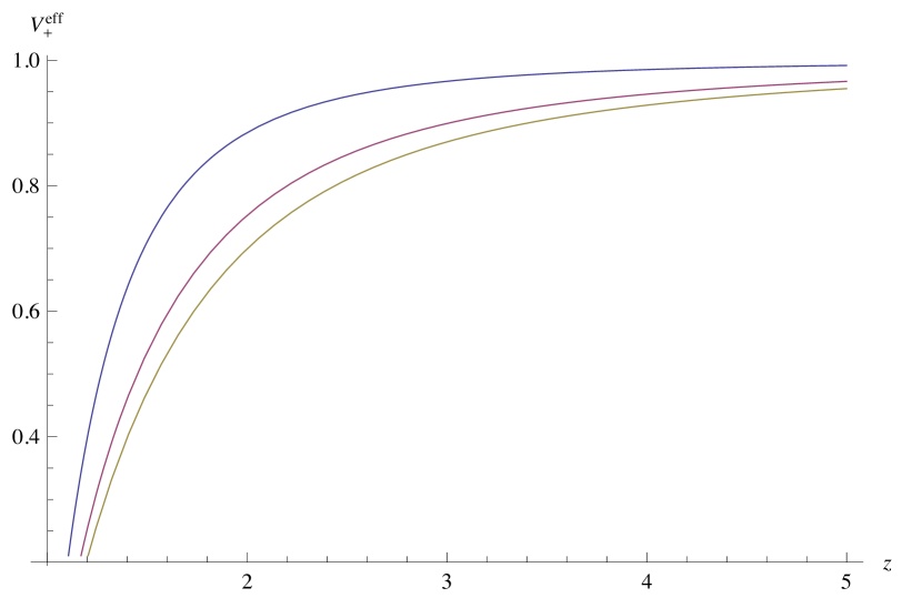
Figure 1: This figure shows $V^{\text{eff}}_{+}(z)$ for fixed $v=0.10,\,\mathfrak{m}^{2}=1.00,\,\delta h=0.06$, and three different values of $\delta g=0.50,\,7.00,\,10.00$. As $\delta g$ increases the potential increases faster towards the boundary where it reaches a local maximum with $V_{+}^{\text{eff}}(z=\infty)=1$.

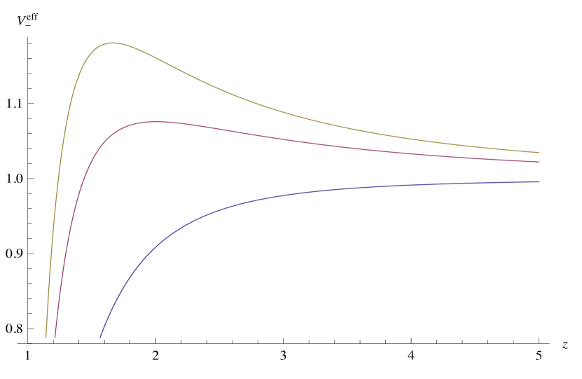
Figure 2: Here we see a plot of $V_{-}^{\text{eff}}(z)$ versus $z$ for fixed $v=0.10,\,\mathfrak{m}^{2}=1.00,\,\delta h=0.06$, and for $\delta g=0.50,\,7.00,\,10.00$. When $\delta g^{2}$ becomes greater than $\mathfrak{m}^{2}$ the potential attains a local maximum whose value exceeds unity.

It is instructive to study how $V_{\pm}^{\text{eff}}$ change as $\delta g$ and $\delta h$ are varied. A plot of the effective potential of each mode for various values of $\delta g$ where $\delta h$ and $\mathfrak{m}$ are held fixed, is presented in Fig. 1 and Fig. 2 . On the one hand, $V^{\text{eff}}_{+}$ smoothly decreases except for a tiny region close to the horizon, as expected from (33). $V^{\text{eff}}_{-}$, on the other hand, develops a local maximum with $\text{Sup}\left\{V^{\text{eff}}_{-}\right\}>1$ for some values of $\delta g$. In this case the existence of a turning point for $E>1$ is unambiguous and the potential supports metastable states whose group velocity may exceed unity.

To examine the conditions under which causality is violated let us first expand the effective potential near the boundary:

$$V^{\text{eff}}_{-}=1+\frac{2v}{z^{2}}\left[\frac{|\delta g|}{\sqrt{\mathfrak{m}^{2}}}-1\right]-\frac{3}{z^{4}}\left[1-\frac{v^{2}}{3}\left(\left[\frac{|\delta g|}{\sqrt{\mathfrak{m}^{2}}}-1\right]^{2}+\frac{\delta g^{2}}{\mathfrak{m}^{2}}+\frac{2\delta g}{\mathfrak{m}^{2}}\right)\right]+\mathcal{O}\left(\frac{1}{z^{6}}\right).$$ (34)

We see that whenever $\delta g^{2}>\mathfrak{m}^{2}$, even for $v\ll 1$, the potential will develop a maximum. As long as the coefficient of the $\mathcal{O}(v^{2})$ term is not too large, the first three terms in the near-boundary expansion (34) suffice to give an estimation of the maximum of the potential. This in turn enables one to compute the group velocity (30), which has the following power-series expansion in $v$:

$$u_{g}=1+v-\frac{v^{2}}{6}\left(\frac{|\delta g|}{\sqrt{\mathfrak{m}^{2}}}-1\right)^{2}+\mathcal{O}(v^{4}).$$ (35)

It is clear that for $v\ll 1$ the group velocity always exceeds unity for finite values of $\delta g^{2}/\mathfrak{m}^{2}$. Causality violation can be avoided by forbidding the potential to develop a maximum with the condition:

$$\delta g^{2}~{}\leq~{}\mathfrak{m}^{2}.$$ (36)

Note that if $v$ ceases to be small, the effective potential might develop a maximum even for values of $\delta g^{2}$ within the bound (36). This however does not necessarily imply causality violation since the group velocity may still remain smaller than unity. In any case, analyzing this regime of $v$ is beyond the scope this article.

3 Conclusions & Outlook

In this paper, we have shown that holography constrains the EM and gravitational couplings of a spin-1 field. For a given mass, the otherwise undetermined $g$-factor and $h$-factor of the classical theory are allowed to take values only in some given range. The results followed from considering in AdS Reissner-Nordström background the dynamics of spin-1 fluctuations, whose EoMs simplify in a certain region of the parameter space, so that one could employ the WKB method to construct explicit solutions. For the modes coupled to the dual boundary operator, one could then calculate the group velocity, which become superluminal unless the spin-1 couplings are constrained.

Field theoretically, the Lagrangian (2) describes generic electromagnetic and gravitational couplings of a massive vector boson. The bounds (32) and (36), however, are obtained for a very particular setup $-$ when the spin 1 is a probe in a dynamical Maxwell-Einstein background with the AdS Reissner-Nordström geometry, so that holography could be employed. The generic situation of an arbitrary background may not come with a holographic interpretation, but is likely to call for sharper bounds. Since the couplings $q$, $g$, $h$ and the original mass $m^{2}$ (which one takes to be positive) appearing in the Lagrangian (2) are a priori independent of one another, one expects the same for the bounds on these couplings. This possibility leads to the “natural” value of $g=2$ and to $h\leq 1$.

It is quite possible that a more extensive holographic analysis, which takes into consideration other regions of the parameter space, could yield stronger constraints. From the point of view of the CFT, the constraints obtained here on $\delta g$ presumably correspond to unitarity constraints on the parameters that determine the 3-point function of two spin-1 operators and a conserved vector current (or stress energy tensor operator) [14, 15]. After all, their holographic derivation is remarkably similar to that appearing in [9]. The black hole background used in [9] to provide a non-zero expectation value for the stress energy tensor operator, is replaced here by the Reissner-Nordström which provides a non-zero charge density (or chemical potential). While Ref. [9] studied the 2-point function of the stress energy tensor, in this work we consider the 2-point function of a non-conserved spin-1 operator.

Given this interpretation, one could try to reproduce our results in field theory by following the reasoning of [15]. Consider for example the 2-point function of a spin-1 operator at finite charge density $\rho\equiv\langle J_{t}\rangle$ with the help of the operator product expansion (ope),

$$\langle\mathcal{O}_{\mu}(-k)\mathcal{O}_{\nu}(k)\rangle=\cdots+\mathcal{A}_{\mu\nu}^{~{}~{}\;\sigma}(k)\langle J_{\sigma}\rangle+\cdots\,,$$ (37)

where the dots represent the contribution of other operators in the ope. Symmetries imply that the ope coefficient $\mathcal{A}_{\mu\nu\sigma}$ can only depend on a few (generically coupling constant dependent) parameters. Moreover it is possible to show that in the large frequency and large momentum limit, i.e., when ${\omega\over\rho}\gg 1$ and ${k\over\rho}\gg 1$ the term explicitly shown in (37) provides the leading contribution to the 2-point function. Positivity of the spectral density of the 2-point function will then necessarily impose constraints on the parameters which appear in $\mathcal{A}_{\mu\nu\sigma}(k)$.

However, there is an obvious issue with this line of reasoning. Unlike the thermal expectation value of the stress energy tensor which is necessarily positive definite (since it is the energy of the system), the charge density expectation value can have either sign. The same issue arises if we try to interpret these constraints as charge flux constraints in analogy with the energy flux constraints of [14]. The charge flux operator was already defined in [14] but to the best of our knowledge there is no physical principle which would restrict its 1-point functions to be non-negative. Perhaps the resolution of this puzzle lies in understanding the parameter-space region where the results are derived $-$ as one can see from (18), the chemical potential is scaled with the momentum in the large momentum region. It would be interesting to investigate this point further and give a proper identification of the couplings $g$ and $h$ in terms of the dual CFT.

We emphasize again that the parameters which determine the 3-point function of two spin-1 operators and a conserved current are in general ’t Hooft coupling dependent . Hence if the cubic couplings discussed here correspond to these CFT parameters, Eqs. (36) and (32) would represent constrains at strong coupling. In this respect our results may have some predictive value, especially since consistency of the dual CFT for spin-1 operators of arbitrary conformal dimension requires that $\delta g=0$ .

In this work we have seen that for a bulk theory which is perfectly consistent classically, the boundary dual may be inconsistent. Could it be that the CFT actually probes the quantum consistency of the theory in the bulk? An affirmative answer might find justification in the fact that perturbative renormalizability of the spin-1 electrodynamics indeed requires the $g$-factor to be constrained (to the bare value of 2) [20]. Classically consistent in $\text{AdS}_{3}$, some Vasiliev-like theories also seem to support this, since they are believed to lack a healthy quantum description and the corresponding CFT is known to be non-unitary [39] . One might therefore argue that the duality holds good if the full quantum theory in the bulk, at least in the weak coupling regime, is well behaved. As we have already mentioned, weak coupling requires $g\approx 2$ for all spin [23].

One might wonder what would be the consequences of other possible cubic couplings added to the Lagrangian (2). At the 2-derivative level, indeed, there is the non-minimal coupling to the scalar curvature: $RW^{\ast}_{\mu}W^{\mu}$. This term redefines the effective mass, but has no contribution to the gravitational quadrupole [31, 33]. Inclusion of this term would not affect our analysis, and we have chosen to drop it for the sake of simplicity. Among the possible higher-derivative cubic couplings the only one relevant for our analysis is the ad hoc 3-derivative EM quadrupole term: $W^{*}_{\mu}\nabla^{\mu}F^{\nu\rho}\nabla_{\nu}W_{\rho}+\text{h.c.}$, which alters the value of $Q_{e}$ given in Eq. (1). But such a term is inconsistent to begin with, since it afflicts the classical bulk theory with superluminal modes [18].

In principle, for particles of any spin one should be able to do similar analysis to constrain their EM and gravitational couplings. Spin $\tfrac{1}{2}$ is particularly interesting in this respect because it has a striking similarity with spin 1: the classical electrodynamics of either particle allows an arbitrary $g$-factor but quantum consistency (perturbative renormalizability) of the theory requires in either case that $g=2$. It was recently appreciated that cubic couplings for a spin-$\tfrac{1}{2}$ field show up naturally in top-down AdS/CFT models [40, 41, 42, 43]. In these class of models, the $g$-factor for given mass and charge of the fermion can take several discrete values ^,.

One would also like to study higher spins, for which the bulk theory is generically fraught with inconsistencies already at the classical level [18, 27, 28, 29]. One might consider, for example, the next simple case of a spin-2 field $\varphi_{\mu\nu}$, for which the $g$- and $h$-factors appear the Lagrangian in the following way.

$$\mathcal{L} = -|\nabla_{\mu}\varphi_{\nu\rho}|^{2}+2|\nabla_{\mu}\varphi^{\mu\nu}|^{2}+|\nabla_{\mu}\varphi|^{2}+\left(\varphi^{\ast}_{\mu\nu}\nabla^{\mu}\nabla^{\nu}\varphi+\text{c.c.}\right)-m^{2}\left(|\varphi_{\mu\nu}|^{2}-|\varphi|^{2}\right)$$ (38)

$$+2iqgF^{\mu\nu}\varphi^{\ast}_{\mu\rho}\varphi_{\nu}^{\rho}+2h\varphi^{\ast}_{\mu\nu}\left(R_{\mu\alpha\nu\beta}\varphi^{\alpha\beta}-R^{\mu\alpha}\varphi_{\alpha}^{\nu}\right)+...\,,$$

where $\varphi^{\mu}_{\mu}\equiv\varphi$, and the ellipses stand for non-minimal terms that are not important for our purpose . Here we expect that $g$ and $h$ will be constrained as well, just as they are for the spin-1 field. It is worth mentioning that recently a spin-2 action in $\text{AdS}_{5}$ was derived by consistent truncation of type IIB supergravity on an Einstein-Sasaki manifold, where the gyromagnetic ratio does not take the natural value of 2 [43]. It will be interesting to see what implications the pathologies of the classical theory in the bulk may have for the dual CFT. We leave these as future work.

Acknowledgments

We would like to thank R. Argurio, A. Parnachev and M. Taylor for useful discussions. The work of MK is partially supported by the ERC Advanced Grant “SyDuGraM”, by IISN-Belgium (convention 4.4514.08) and by the “Communauté Française de Belgique” through the ARC program. RR is a Postdoctoral Fellow of the Fonds de la Recherche Scientifique-FNRS. His work is partially supported by IISN-Belgium (conventions 4.4511.06 and 4.4514.08) and by the “Communauté Française de Belgique” through the ARC program.

Appendix A Stability Bound in AdS

In pure $\text{AdS}_{d+1}$, let us consider a massive vector field that does not backreact on the geometry. The dynamical background satisfies the EoM

$$R^{\mu\nu}=-dg^{\mu\nu},$$ (A.1)

which simplifies the last term in the spin-1 action (2), and reduce it to

$$\mathcal{S}=\int d^{d+1}x\,\sqrt{-g}\,\Big{(}-\tfrac{1}{2}\mathcal{F}_{\mu\nu}^{*}\mathcal{F}^{\mu\nu}-\mathfrak{m}^{2}W_{\mu}^{*}W^{\mu}\Big{)},$$ (A.2)

where $\mathcal{F}_{\mu\nu}\equiv\nabla_{\mu}W_{\nu}-\nabla_{\nu}W_{\mu}$ is the spin-1 curvature, and $\mathfrak{m}^{2}\equiv m^{2}-d(h-1)$ is the effective mass in AdS. One can show that

$$\mathfrak{m}^{2}~{}\geq~{}0,$$ (A.3)

if the energy functional for $W_{\mu}$ is required to be positive definite . Apart from the fact that a generic non-zero value of $h-1$ changes the effective mass, the proof is essentially given in Appendix B of [45], which we rephrase here for the sake of self-containedness.

The stress-energy tensor for the spin-1 field is

$$\mathcal{T}_{\mu\nu}=\frac{2}{\sqrt{-g}}\,\frac{\delta\mathcal{S}}{\delta g^{\mu\nu}}\,,$$ (A.4)

which, when integrated over a spacelike slice orthogonal to the timelike Killing vector $\xi^{\mu}=(1,0,\dots,0)$, gives the energy functional

$$\mathcal{E}=\int d^{d}x\,\sqrt{-g}\,\mathcal{T}^{0\mu}\xi_{\mu}.$$ (A.5)

To compute this quantity, one can choose the line element

$$ds^{2}=(1/\cosh^{2}\rho)(-dt^{2}+d\rho^{2}+\sinh^{2}\rho\,d\Omega_{d-1}),$$ (A.6)

and distinguish the time component ($\mu=0$) from the spatial ones ($\mu,\nu=i,j$). One finds that the energy functional (A.5) boils down to

$$\mathcal{E}=\int d^{d}x\,\tanh^{d-1}\rho\,\left[g^{ij}\mathcal{F}_{0i}^{*}\mathcal{F}_{0j}+\frac{1}{2\cosh^{2}\rho}\,\mathcal{F}_{ij}^{*}\mathcal{F}^{ij}+\mathfrak{m}^{2}|W_{0}|^{2}+\frac{\mathfrak{m}^{2}}{\cosh^{2}\rho}\,W_{i}^{*}W^{i}\right].$$ (A.7)

Note that $\mathcal{F}_{\mu\nu}=0$ is always a valid solution, even when $\mathfrak{m}^{2}\neq 0$. To see this, one notices that the energy functional (A.7) depends on neither $\partial_{0}W_{0}$ nor $\partial_{\rho}W_{\rho}$. Therefore, at a given time one can construct modes with only one non-zero component: $W_{\rho}(\rho)$, which vanishes at large $\rho$ arbitrarily fast and satisfies $\partial_{0}W_{\rho}=0$. When $\mathfrak{m}^{2}\neq 0$, there appears the constraint $\nabla\cdot W=0$, but it merely fixes the quantity $\partial_{0}W_{0}$.

Given this, if we demand that $\mathcal{E}$ be positive definite, restrictions on $\mathfrak{m}^{2}$ follow immediately. When $\mathfrak{m}^{2}>0$, the energy functional (A.7) is manifestly positive definite. When $\mathfrak{m}^{2}=0$, solutions with $\mathcal{F}_{\mu\nu}=0$ have zero energy, so that $\mathcal{E}$ is semi-positive definite. However, because energy is interpreted as the norm in the Hilbert space of states, such solutions are unphysical and correspond to null states. If $\mathfrak{m}^{2}<0$, the energy functional can become negative, which is obviously the case for solutions with $\mathcal{F}_{\mu\nu}=0$. Correspondingly, the Hilbert space is plagued with negative-norm states. This sets the bound (A.3).

Appendix B The Spin-1 EoMs

Under the limit (18), the EoMs for the modes $\mathcal{E}_{i}$ reduce to (19), which contain the functions $a(z)$, $b(z)$, $c(z)$ and $d(z)$, whose explicit forms are given below.

$$a(z) = 2\delta g\,vz^{3}N_{1}^{-1}(z),$$ (B.1)

$$b(z) = \tfrac{z^{2}N_{1}(z)}{\left(z^{2}-1\right)^{4}\left(z^{2}+2\right)^{2}}\,,$$ (B.2)

$$c(z) = 2\delta g\,vzN_{2}^{-1}(z),$$ (B.3)

$$d(z) = -\tfrac{4\delta g^{2}v^{2}z^{6}(z^{2}-1)^{2}(z^{2}+2)((u-v)z^{2}+v)^{2}+4\delta g\,v^{2}z^{4}(z^{2}-1)^{2}(z^{2}+2)N_{1}(z)+z^{2}N_{1}(z)N_{3}(z)}{\left(z^{2}-1\right)^{3}\left(z^{2}+2\right)\left(z^{4}+z^{2}-2\right)N_{1}(z)N_{2}(z)}\,,$$ (B.4)

where the functions $N_{1}(z)$, $N_{2}(z)$ and $N_{3}(z)$ are defined as

$$N_{1}(z) = z^{6}\left[(u-v)^{2}-1\right]+2z^{4}v(u-v)+z^{2}(v^{2}+3)-2,$$

$$N_{2}(z) = \mathfrak{m}^{2}z^{6}-8\delta h,$$ (B.5)

$$N_{3}(z) = 4\delta{h}\left[z^{6}\left(2(u-v)^{2}+1\right)+4z^{4}v(u-v)+z^{2}(2v^{2}-3)+2\right]-\mathfrak{m}^{2}z^{6}N_{1}(z).$$

Appendix C Turning Points

First we show that there exist no turning points of the second class, defined in (27). In other words, we show that the polynomial below–the square root in Eq. (25)–has no real solution for $z>1$. In the following, we set $z^{2}=y$ and define the polynomial in question

$$Z(y)\equiv v^{2}\mathfrak{m}^{2}\delta g^{2}\left[y^{4}+{\left(1+\delta g\right)^{2}v^{2}\over\mathfrak{m}^{2}}\,y^{2}+2\delta h{\left(3-\delta g\right)\over\delta g\,\mathfrak{m}^{2}}\,y+{9\delta h^{2}\over\delta g^{2}v^{2}\mathfrak{m}^{2}}\right]$$ (C.1)

Notice first that $Z(y)$ behaves like $y^{4}$ near the boundary and is non-negative at the horizon $y=1$. For the allowed values of $\delta h$, i.e., $-\tfrac{1}{4}\mathfrak{m}^{2}\leq\delta h<\tfrac{1}{8}\mathfrak{m}^{2}$, it is in fact possible to show that $Z(y)$ is non-negative everywhere in the bulk for $y>1$. This implies that any real roots outside the horizon will coincide with a point where $Z(y)$ has a minimum. In other words, any root should also be a root of the derivative of the polynomial. From Descartes rule of signs, one sees that $Z(y)$ will generically have only complex roots. It is only when the coefficient of the linear term in (C.1) is negative and the following inequalities are met, namely,

$$\begin{split}&\delta h>0\quad\&\quad 0>\delta g>{-3\delta h\,\over 2\mathfrak{m}^{2}-\delta h}\quad\&\quad|v|<\sqrt{\frac{-2\delta g\,\mathfrak{m}^{2}-\delta h\left(3-\delta g\right)}{\delta g\left(1+\delta g\right)^{2}}}\,,\\ &\delta h<0\quad\&\quad 0<\delta g<{-3\delta h\,\over 2\mathfrak{m}^{2}-\delta h}\quad\&\quad|v|<\sqrt{\frac{-2\delta g\,\mathfrak{m}^{2}-\delta h\left(3-\delta g\right)}{\delta g\left(1+\delta g\right)^{2}}}\,,\\ \end{split}$$ (C.2)

may the polynomial have two real roots outside the horizon. Since every such root of $Z(y)$ must also be a root of $Z^{\prime}(y)$, and $Z^{\prime}(y)$ is a cubic polynomial with just one real root, the only possibility is that $Z(y)$ has a double real root. However, this is only true if a relation exists between the coefficients of the polynomial which cannot be satisfied for generic $\delta g\neq 0,\,v\neq 0$. As a result there are no second class turning points.

Next, we would like to show that $\left(\partial{\mathbb{G}}\over\partial u\right)$ and $\left(\partial{\mathbb{G}}\over\partial v\right)$ are non-vanishing when evaluated at the turning point $z_{t}$. Recall that we consider the turning point $z_{t}$ which is closest to the boundary $z=\infty$ and where

$$p^{2}(z_{t})\equiv\tfrac{1}{2}\left(-\left[a(z)c(z)-b(z)-d(z)\right]\pm\sqrt{\left[a(z)c(z)-b(z)-d(z)\right]^{2}-4b(z)d(z)}\right)_{z=z_{t}}=0\,.$$ (C.3)

The explicit form of the functions $a(z)$, $b(z)$, $c(z)$, $d(z)$ can be found in Appendix B. Given that these functions are real, Eq. (C.3) essentially implies that the turning point will be a solution of the equation $b(z)d(z)=0$.

The determinant $\mathbb{G}$ is now defined as

$${\mathbb{G}}\equiv p^{4}+p^{2}\left[a(z)c(z)-b(z)-d(z)\right]+b(z)d(z)\,,$$ (C.4)

It follows that

$${\partial\mathbb{G}\over\partial u}=p^{2}{\partial\over\partial u}\left[a(z)c(z)-b(z)-d(z)\right]+{\partial\over\partial u}\,b(z)d(z).$$ (C.5)

Evaluated at the turning point $z=z_{t}$, where $p^{2}(z_{t})=0$, Eq. (C.5) reduces to

$$\left(\partial\mathbb{G}\over\partial u\right)=\left.{\partial\over\partial u}\,b(z)d(z)\right|_{z=z_{t}}\,.$$ (C.6)

With the help of Appendix B, it is easy to deduce that

$$b(z)d(z)=P^{-1}(z)\left[u^{4}P_{4}(z)+u^{3}P_{3}(z)+u^{2}P_{2}(z)+uP_{1}(z)+P_{0}(z)\right],$$ (C.7)

where $P(z),\,P_{i}(z)$ with $i=1,...,4$ are polynomials of $z$, and $P(z)$ diverges like $z^{8}$ at the boundary. Since $b(z)d(z)$ is a polynomial in $u$ it can also be written as

$$b(z)d(z)=P^{-1}(z)P_{4}(z)\left(u-u_{1}(z)\right)\left(u-u_{2}(z)\right)\left(u-u_{3}(z)\right)\left(u-u_{4}(z)\right).$$ (C.8)

At the turning point under consideration some but not all of the parentheses may vanish so that (C.6) is finite and different from zero. In a similar manner one can show that ${\partial{\mathbb{G}}\over\partial v}\neq 0$. Finally let us note for completeness that ${\partial\mathbb{G}\over\partial p}$ behaves like $z^{-8}$ close to the boundary and thus ${\partial p\over\partial u}$ is finite there.

References

- [1] J. M. Maldacena, Adv. Theor. Math. Phys. 2, 231 (1998) [hep-th/9711200].
- [2] S. S. Gubser, I. R. Klebanov and A. M. Polyakov, Phys. Lett. B 428, 105 (1998) [hep-th/9802109].
- [3] E. Witten, Adv. Theor. Math. Phys. 2, 253 (1998) [hep-th/9802150].
- [4] S. Deser and A. Waldron, Phys. Lett. B 513, 137 (2001) [hep-th/0105181]; Nucl. Phys. B 607, 577 (2001) [hep-th/0103198]; Phys. Lett. B 508, 347 (2001) [hep-th/0103255]; Phys. Rev. Lett. 87, 031601 (2001) [hep-th/0102166]. S. Deser and R. I. Nepomechie, Annals Phys. 154, 396 (1984); Phys. Lett. B 132, 321 (1983).
- [5] A. Higuchi, Nucl. Phys. B 325, 745 (1989); Nucl. Phys. B 282, 397 (1987); Class. Quant. Grav. 6, 397 (1989).
- [6] I. L. Buchbinder, D. M. Gitman and V. D. Pershin, Phys. Lett. B 492, 161 (2000) [hep-th/0006144]. I. L. Buchbinder, D. M. Gitman, V. A. Krykhtin and V. D. Pershin, Nucl. Phys. B 584, 615 (2000) [hep-th/9910188].
- [7] L. Dolan, C. R. Nappi and E. Witten, JHEP 0110, 016 (2001) [hep-th/0109096].
- [8] C. Lanczos Z. Phys. 73, 147 (1932). C. Lanzcos Ann. Math. 39, 842 (1938). D. Lovelock, J. Math. Phys. 12, 498 (1971).
- [9] M. Brigante, H. Liu, R. C. Myers, S. Shenker and S. Yaida, Phys. Rev. Lett. 100, 191601 (2008) [arXiv:0802.3318 [hep-th]]; Phys. Rev. D 77, 126006 (2008) [arXiv:0712.0805 [hep-th]].
- [10] A. Buchel and R. C. Myers, JHEP 0908, 016 (2009) [arXiv:0906.2922 [hep-th]].
- [11] D. M. Hofman, Nucl. Phys. B 823, 174 (2009) [arXiv:0907.1625 [hep-th]].
- [12] A. Buchel, J. Escobedo, R. C. Myers, M. F. Paulos, A. Sinha and M. Smolkin, JHEP 1003, 111 (2010) [arXiv:0911.4257 [hep-th]]. J. de Boer, M. Kulaxizi and A. Parnachev, JHEP 1003, 087 (2010) [arXiv:0910.5347 [hep-th]]. X. O. Camanho and J. D. Edelstein, JHEP 1004, 007 (2010) [arXiv:0911.3160 [hep-th]].
- [13] J. de Boer, M. Kulaxizi and A. Parnachev, JHEP 1006, 008 (2010) [arXiv:0912.1877 [hep-th]]. X. O. Camanho and J. D. Edelstein, JHEP 1006, 099 (2010) [arXiv:0912.1944 [hep-th]]. X. O. Camanho, J. D. Edelstein and M. F. Paulos, JHEP 1105, 127 (2011) [arXiv:1010.1682 [hep-th]]. R. C. Myers, M. F. Paulos and A. Sinha, JHEP 1008, 035 (2010) [arXiv:1004.2055 [hep-th]].
- [14] D. M. Hofman and J. Maldacena, JHEP 0805, 012 (2008) [arXiv:0803.1467 [hep-th]].
- [15] M. Kulaxizi and A. Parnachev, Phys. Rev. Lett. 106, 011601 (2011) [arXiv:1007.0553 [hep-th]].
- [16] C. Lorce, Phys. Rev. D 79, 113011 (2009) [arXiv:0901.4200 [hep-ph]].
- [17] H. Aronson, Phys. Rev. 186, 1434 (1969).
- [18] G. Velo and D. Zwanziger, Phys. Rev. 188, 2218 (1969).
- [19] S. J. Brodsky and J. R. Hiller, Phys. Rev. D 46, 2141 (1992).
- [20] J. M. Cornwall, D. N. Levin and G. Tiktopoulos, Phys. Rev. Lett. 30, 1268 (1973) [Erratum-ibid. 31, 572 (1973)]; Phys. Rev. D 10, 1145 (1974) [Erratum-ibid. D 11, 972 (1975)].
- [21] W. A. Bardeen, R. Gastmans and B. E. Lautrup, Nucl. Phys. B 46, 319 (1972).
- [22] K. J. Kim and Y. -S. Tsai, Phys. Rev. D 7, 3710 (1973).
- [23] S. Weinberg, Lectures On Elementary Particles And Quantum Field Theory, Proceedings of the Summer Institute, Brandeis University, 1970, Vol. I, (MIT Press, Cambridge, MA, 1970).
- [24] S. Ferrara, M. Porrati and V. L. Telegdi, Phys. Rev. D 46, 3529 (1992).
- [25] S. Ferrara and M. Porrati, Phys. Lett. B 288, 85 (1992).
- [26] P. C. Argyres and C. R. Nappi, Phys. Lett. B 224, 89 (1989). M. Porrati, R. Rahman and A. Sagnotti, Nucl. Phys. B 846, 250 (2011) [arXiv:1011.6411 [hep-th]].
- [27] G. Velo and D. Zwanziger, Phys. Rev. 186, 1337 (1969). G. Velo, Nucl. Phys. B 43, 389 (1972).
- [28] A. Shamaly, A. Z. Capri, Annals Phys. 74, 503-523 (1972); Can. J. Phys. 52, 919-920 (1974). M. Hortacsu, Phys. Rev. D 9, 928 (1974). J. Prabhakaran, M. Seetharaman, P. M. Mathews, Phys. Rev. D12, 3191-3194 (1975); Phys. Rev. D12, 458-466 (1975); J. Phys. A A8, 560-565 (1975).
- [29] S. Deser, V. Pascalutsa and A. Waldron, Phys. Rev. D 62, 105031 (2000) [arXiv:hep-th/0003011]. S. Deser and A. Waldron, Nucl. Phys. B 631, 369 (2002) [arXiv:hep-th/0112182].
- [30] M. Porrati and R. Rahman, Phys. Rev. D 80, 025009 (2009) [arXiv:0906.1432 [hep-th]]. R. Rahman, arXiv:1111.3366 [hep-th].
- [31] I. Giannakis, J. T. Liu and M. Porrati, Phys. Lett. B 469, 129 (1999) [hep-th/9909012].
- [32] I. B. Khriplovich, Sov. Phys. JETP 69, 217 (1989) [Zh. Eksp. Teor. Fiz. 96, 385 (1989)]. I. B. Khriplovich and A. A. Pomeransky, J. Exp. Theor. Phys. 86, 839 (1998) [Zh. Eksp. Teor. Fiz. 113, 1537 (1998)] [gr-qc/9710098]; Surveys High Energ. Phys. 14, 145 (1999) [gr-qc/9809069].
- [33] M. Porrati, Phys. Lett. B 304, 77 (1993) [gr-qc/9301012]. A. Cucchieri, M. Porrati and S. Deser, Phys. Rev. D 51, 4543 (1995) [hep-th/9408073].
- [34] L. J. Romans, Nucl. Phys. B 383, 395 (1992) [hep-th/9203018]. A. Chamblin, R. Emparan, C. V. Johnson and R. C. Myers, Phys. Rev. D 60, 064018 (1999) [hep-th/9902170].
- [35] K. Yabana and H. Horiuchi, Prog. Theor. Phys. 71, 1275 (1984); Prog. Theor. Phys. 75, 592 (1986).
- [36] T. Faulkner, H. Liu, J. McGreevy and D. Vegh, Phys. Rev. D 83, 125002 (2011) [arXiv:0907.2694 [hep-th]].
- [37] R. C. Myers, A. O. Starinets and R. M. Thomson, JHEP 0711, 091 (2007) [arXiv:0706.0162 [hep-th]].
- [38] X. H. Ge and S. J. Sin, JHEP 0905, 051 (2009) [arXiv:0903.2527 [hep-th]]. X. H. Ge, Y. Matsuo, F. W. Shu, S. J. Sin and T. Tsukioka, JHEP 0810, 009 (2008) [arXiv:0808.2354 [hep-th]]. R. G. Cai, Z. Y. Nie and Y. W. Sun, Phys. Rev. D 78, 126007 (2008) [arXiv:0811.1665 [hep-th]]. R. G. Cai, Z. Y. Nie, N. Ohta and Y. W. Sun, Phys. Rev. D 79, 066004 (2009) [arXiv:0901.1421 [hep-th]].
- [39] E. Perlmutter, T. Prochazka and J. Raeymaekers, arXiv:1210.8452 [hep-th].
- [40] M. Ammon, J. Erdmenger, M. Kaminski and A. O’Bannon, JHEP 1005, 053 (2010) [arXiv:1003.1134 [hep-th]].
- [41] I. Bah, A. Faraggi, J. I. Jottar, R. G. Leigh and L. A. Pando Zayas, JHEP 1102, 068 (2011) [arXiv:1008.1423 [hep-th]]. I. Bah, A. Faraggi, J. I. Jottar and R. G. Leigh, JHEP 1101, 100 (2011) [arXiv:1009.1615 [hep-th]].
- [42] O. DeWolfe, S. S. Gubser and C. Rosen, Phys. Rev. Lett. 108, 251601 (2012) [arXiv:1112.3036 [hep-th]]. O. DeWolfe, S. S. Gubser and C. Rosen, Phys. Rev. D 86, 106002 (2012) [arXiv:1207.3352 [hep-th]].
- [43] K. -Y. Kim and M. Taylor, arXiv:1304.6729 [hep-th]. M. Taylor, Talk at “Holography, Gauge Theory and Black Holes” Workshop, Amsterdam, 17-19 Dec. 2012.
- [44] M. Edalati, R. G. Leigh and P. W. Phillips, Phys. Rev. Lett. 106, 091602 (2011) [arXiv:1010.3238 [hep-th]]. M. Edalati, R. G. Leigh, K. W. Lo and P. W. Phillips, Phys. Rev. D 83, 046012 (2011) [arXiv:1012.3751 [hep-th]]. D. Guarrera and J. McGreevy, arXiv:1102.3908 [hep-th].
- [45] F. Benini, C. P. Herzog, R. Rahman and A. Yarom, JHEP 1011, 137 (2010) [arXiv:1007.1981 [hep-th]].
- [46] P. Breitenlohner and D. Z. Freedman, Phys. Lett. B 115, 197 (1982).