Cluster algebras: an introduction

Abstract.

Cluster algebras are commutative rings with a set of distinguished generators having a remarkable combinatorial structure. They were introduced by Fomin and Zelevinsky in 2000 in the context of Lie theory, but have since appeared in many other contexts, from Poisson geometry to triangulations of surfaces and Teichmüller theory. In this expository paper we give an introduction to cluster algebras, and illustrate how this framework naturally arises in Teichmüller theory. We then sketch how the theory of cluster algebras led to a proof of the Zamolodchikov periodicity conjecture in mathematical physics.

1. Introduction

Cluster algebras were conceived by Fomin and Zelevinsky [13] in the spring of 2000 as a tool for studying total positivity and dual canonical bases in Lie theory. However, the theory of cluster algebras has since taken on a life of its own, as connections and applications have been discovered to diverse areas of mathematics including quiver representations, Teichmüller theory, tropical geometry, integrable systems, and Poisson geometry.

In brief, a cluster algebra $\mathcal{A}$ of rank $n$ is a subring of an ambient field $\mathcal{F}$ of rational functions in $n$ variables. Unlike “most” commutative rings, a cluster algebra is not presented at the outset via a complete set of generators and relations. Instead, from the initial data of a seed – which includes $n$ distinguished generators called cluster variables plus an exchange matrix – one uses an iterative procedure called mutation to produce the rest of the cluster variables. In particular, each new cluster variable is a rational expression in the initial cluster variables. The cluster algebra is then defined to be the subring of $\mathcal{F}$ generated by all cluster variables.

The set of cluster variables has a remarkable combinatorial structure: this set is a union of overlapping algebraically independent $n$-subsets of $\mathcal{F}$ called clusters, which together have the structure of a simplicial complex called the cluster complex. The clusters are related to each other by birational transformations of the following kind: for every cluster $\mathbf{x}$ and every cluster variable $x\in\mathbf{x}$, there is another cluster $\mathbf{x}^{\prime}=(\mathbf{x}-\{x\})\cup\{x^{\prime}\}$, with the new cluster variable $x^{\prime}$ determined by an exchange relation of the form

$$xx^{\prime}=y^{+}M^{+}+y^{-}M^{-}.$$

Here $y^{+}$ and $y^{-}$ lie in a coefficient semifield $\mathbb{P}$, while $M^{+}$ and $M^{-}$ are monomials in the elements of $\mathbf{x}-\{x\}$. In the most general class of cluster algebras, there are two dynamics at play in the exchange relations: that of the monomials, and that of the coefficients, both of which are encoded in the exchange matrix.

The aim of this article is threefold: to give an elementary introduction to the theory of cluster algebras; to illustrate how the framework of cluster algebras naturally arises in diverse areas of mathematics, in particular Teichmüller theory; and to illustrate how the theory of cluster algebras has been an effective tool for solving outstanding conjectures, in particular the Zamolodchikov periodicity conjecture from mathematical physics.

To this end, in Section 2 we introduce the notion of cluster algebra, beginning with the simple but somewhat restrictive definition of a cluster algebra defined by a quiver. After giving a detailed example (the type A cluster algebra, and its realization as the coordinate ring of the Grassmannian $Gr_{2,d}$), we give a more general definition of cluster algebra, in which both the cluster variables and coefficient variables have their own dynamics.

In Section 3 we explain how cluster algebras had appeared implicitly in Teichmüller theory, long before the introduction of cluster algebras themselves. We start by associating a cluster algebra to any bordered surface with marked points, following work of Fock-Goncharov [8], Gekhtman-Shapiro-Vainshtein [20], and Fomin-Shapiro-Thurston [11]. This construction specializes to the type A example from Section 2 when the surface is a disk with marked points on the boundary. We then explain how a cluster algebra from a bordered surface is related to the decorated Teichmüller space of the corresponding cusped surface. Finally we briefly discuss the Teichmüller space of a surface with oriented geodesic boundary and two related spaces of laminations, and how natural coordinate systems on these spaces are related to cluster algebras.

In Section 4 we discuss Zamolodchikov’s periodicity conjecture for Y-systems [48]. Although this conjecture arose from Zamolodchikov’s study of the thermodynamic Bethe ansatz in mathematical physics, Fomin-Zelevinsky realized that it could be reformulated in terms of the dynamics of coefficient variables in a cluster algebra [15]. We then discuss how Fomin-Zelevinsky used fundamental structural results for finite type cluster algebras to prove the periodicity conjecture for Dynkin diagrams [15], and how Keller used deep results from the categorification of cluster algebras to prove the corresponding conjecture for pairs of Dynkin diagrams [29, 30].

Acknowledgements: This paper was written to accompany my talk at the Current Events Bulletin Session at the Joint Mathematics Meetings in San Diego, in January 2013; I would like to thank the organizers for the impetus to prepare this document. I gratefully acknowledge the hospitality of MSRI during the Fall 2012 program on cluster algebras, which provided an ideal environment for writing this paper. In addition, I am indebted to Bernhard Keller, Tomoki Nakanishi, and Dylan Thurston for useful conversations, and to Keller for the use of several figures. Finally, I am grateful to an anonymous referee for insightful comments.

2. What is a cluster algebra?

In this section we will define the notion of cluster algebra, first introduced by Fomin and Zelevinsky in [13]. For the purpose of acquainting the reader with the basic notions, in Section 2.1 we will give the simple but somewhat restrictive definition of a cluster algebra defined by a quiver, also called a skew-symmetric cluster algebra of geometric type. We will give a detailed example in Section 2.2, and then present a more general definition of cluster algebra in Section 2.3.

2.1. Cluster algebras from quivers

Definition 2.1 (Quiver).

A quiver $Q$ is an oriented graph given by a set of vertices $Q_{0}$, a set of arrows $Q_{1}$, and two maps $s:Q_{1}\to Q_{0}$ and $t:Q_{1}\to Q_{0}$ taking an arrow to its source and target, respectively.

A quiver $Q$ is finite if the sets $Q_{0}$ and $Q_{1}$ are finite. A loop of a quiver is an arrow $\alpha$ whose source and target coincide. A $2$-cycle of a quiver is a pair of distinct arrows $\beta$ and $\gamma$ such that $s(\beta)=t(\gamma)$ and $t(\beta)=s(\gamma)$.

Definition 2.2 (Quiver Mutation).

Let $Q$ be a finite quiver without loops or $2$-cycles. Let $k$ be a vertex of $Q$. Following [13], we define the mutated quiver $\mu_{k}(Q)$ as follows: it has the same set of vertices as $Q$, and its set of arrows is obtained by the following procedure:

1. for each subquiver $i\to k\to j$, add a new arrow $i\to j$;

2. reverse all allows with source or target $k$;

3. remove the arrows in a maximal set of pairwise disjoint $2$-cycles.

Exercise 2.3.

Mutation is an involution, that is, $\mu_{k}^{2}(Q)=Q$ for each vertex $k$.

Figure 1 shows two quivers which are obtained from each other by mutating at the vertex $1$. We say that two quivers $Q$ and $Q^{\prime}$ are mutation-equivalent if one can get from $Q$ to $Q^{\prime}$ by a sequence of mutations.

Figure 1. Two mutation-equivalent quivers.

Definition 2.4.

Let $Q$ be a finite quiver with no loops or $2$-cycles and whose vertices are labeled $1,2,\dots,m$. Then we may encode $Q$ by an $m\times m$ skew-symmetric exchange matrix $B(Q)=(b_{ij})$ where $b_{ij}=-b_{ji}=\ell$ whenever there are $\ell$ arrows from vertex $i$ to vertex $j$. We call $B(Q)$ the signed adjacency matrix of the quiver.

Exercise 2.5.

Check that when one encodes a quiver $Q$ by a matrix as in Definition 2.4, the matrix $B(\mu_{k}(Q))=(b^{\prime}_{ij})$ is again an $m\times m$ skew-symmetric matrix, whose entries are given by

(2.1) $$b^{\prime}_{ij}=\begin{cases}-b_{ij}&\text{if $i=k$ or $j=k$;}\\[3.61371pt] b_{ij}+b_{ik}b_{kj}&\text{if $b_{ik}>0$ and $b_{kj}>0$;}\\[3.61371pt] b_{ij}-b_{ik}b_{kj}&\text{if $b_{ik}<0$ and $b_{kj}<0$;}\\[3.61371pt] b_{ij}&\text{otherwise.}\end{cases}$$

Definition 2.6 (Labeled seeds).

Choose $m\geq n$ positive integers. Let $\mathcal{F}$ be an ambient field of rational functions in $n$ independent variables over $\mathbb{Q}(x_{n+1},\dots,x_{m})$. A labeled seed in $\mathcal{F}$ is a pair $(\mathbf{x},Q)$, where

• $\mathbf{x}=(x_{1},\dots,x_{m})$ forms a free generating set for $\mathcal{F}$, and

• $Q$ is a quiver on vertices $1,2,\dots,n,n+1,\dots,m$, whose vertices $1,2,\dots,n$ are called mutable, and whose vertices $n+1,\dots,m$ are called frozen.

We refer to $\mathbf{x}$ as the (labeled) extended cluster of a labeled seed $(\mathbf{x},Q)$. The variables $\{x_{1},\dots,x_{n}\}$ are called cluster variables, and the variables $c=\{x_{n+1},\dots,x_{m}\}$ are called frozen or coefficient variables.

Definition 2.7 (Seed mutations).

Let $(\mathbf{x},Q)$ be a labeled seed in $\mathcal{F}$, and let $k\in\{1,\dots,n\}$. The seed mutation $\mu_{k}$ in direction $k$ transforms $(\mathbf{x},Q)$ into the labeled seed $\mu_{k}(\mathbf{x},Q)=(\mathbf{x}^{\prime},\mu_{k}(Q))$, where the cluster $\mathbf{x}^{\prime}=(x^{\prime}_{1},\dots,x^{\prime}_{m})$ is defined as follows: $x_{j}^{\prime}=x_{j}$ for $j\neq k$, whereas $x^{\prime}_{k}\in\mathcal{F}$ is determined by the exchange relation

(2.2) $$x^{\prime}_{k}\ x_{k}=\ \prod_{\begin{subarray}{c}\alpha\in Q_{1}\\ s(\alpha)=k\end{subarray}}x_{t(\alpha)}+\ \prod_{\begin{subarray}{c}\alpha\in Q_{1}\\ t(\alpha)=k\end{subarray}}x_{s(\alpha)}\,.$$

Remark 2.8.

Note that arrows between two frozen vertices of a quiver do not affect seed mutation (they do not affect the mutated quiver or the exchange relation). For that reason, one may omit arrows between two frozen vertices. Correspondingly, when one represents a quiver by a matrix, one often omits the data corresponding to such arrows. The resulting matrix $B$ is hence an $m\times n$ matrix rather than an $m\times m$ one.

Example 2.9.

Let $Q$ be the quiver on two vertices $1$ and $2$ with a single arrow from $1$ to $2$. Let $((x_{1},x_{2}),Q)$ be an initial seed. Then if we perform seed mutations in directions $1$, $2$, $1$, $2$, and $1$, we get the sequence of labeled seeds shown in Figure 2. Note that up to relabeling of the vertices of the quiver, the initial seed and final seed coincide.

Figure 2. Seeds and seed mutations in type $A_{2}$.

Definition 2.10 (Patterns).

Consider the $n$-regular tree $\mathbb{T}_{n}$ whose edges are labeled by the numbers $1,\dots,n$, so that the $n$ edges emanating from each vertex receive different labels. A cluster pattern is an assignment of a labeled seed $\Sigma_{t}=(\mathbf{x}_{t},Q_{t})$ to every vertex $t\in\mathbb{T}_{n}$, such that the seeds assigned to the endpoints of any edge $t\!\begin{array}[]{c}\scriptstyle{k}\\[-7.22743pt] -\!\!\!-\!\!\!-\\[-7.22743pt] {}\scriptstyle\hfil\end{array}\!t^{\prime}$ are obtained from each other by the seed mutation in direction $k$. The components of $\mathbf{x}_{t}$ are written as $\mathbf{x}_{t}=(x_{1;t}\,,\dots,x_{n;t}).$

Clearly, a cluster pattern is uniquely determined by an arbitrary seed.

Definition 2.11 (Cluster algebra).

Given a cluster pattern, we denote

(2.3) $$\mathcal{X}=\bigcup_{t\in\mathbb{T}_{n}}\mathbf{x}_{t}=\{x_{i,t}\,:\,t\in\mathbb{T}_{n}\,,\ 1\leq i\leq n\}\ ,$$

the union of clusters of all the seeds in the pattern. The elements $x_{i,t}\in\mathcal{X}$ are called cluster variables. The cluster algebra $\mathcal{A}$ associated with a given pattern is the $\mathbb{Z}[c]$-subalgebra of the ambient field $\mathcal{F}$ generated by all cluster variables: $\mathcal{A}=\mathbb{Z}[c][\mathcal{X}]$. We denote $\mathcal{A}=\mathcal{A}(\mathbf{x},Q)$, where $(\mathbf{x},Q)$ is any seed in the underlying cluster pattern. In this generality, $\mathcal{A}$ is called a cluster algebra from a quiver, or a skew-symmetric cluster algebra of geometric type. We say that $\mathcal{A}$ has rank $n$ because each cluster contains $n$ cluster variables.

2.2. Example: the type $A$ cluster algebra

In this section we will construct a cluster algebra using the combinatorics of triangulations of a $d$-gon (a polygon with $d$ vertices). We will subsequently identify this cluster algebra with the homogeneous coordinate ring of the Grassmannian $Gr_{2,d}$ of $2$-planes in a $d$-dimensional vector space.

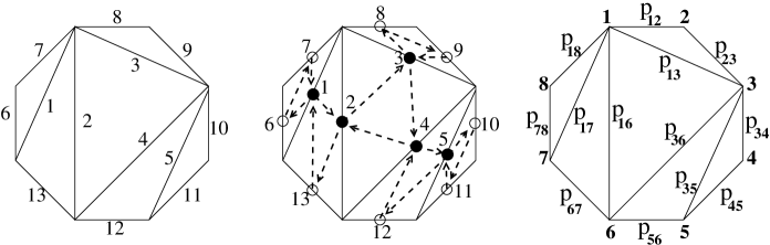
Figure 3. A triangulation $T$ of an octagon, the quiver $Q(T)$, and the labeling of $T$ by Plücker coordinates.

Definition 2.12 (The quiver $Q(T)$).

Consider a $d$-gon $(d\geq 3$), and choose any triangulation $T$. Label the $d-3$ diagonals of $T$ with the numbers $1,2,\dots,d-3$, and label the $d$ sides of the polygon by the numbers $d-2,d-1,\dots,2d-3$. Put a frozen vertex at the midpoint of each side of the polygon, and put a mutable vertex at the midpoint of each diagonal of the polygon. These $2d-3$ vertices are the vertices $Q_{0}(T)$ of $Q(T)$; label them according to the labeling of the diagonals and sides of the polygon. Now within each triangle of $T$, inscribe a new triangle on the vertices $Q_{0}(T)$, whose edges are oriented clockwise. The edges of these inscribed triangles comprise the set of arrows $Q_{1}(T)$ of $Q(T)$.

See the left and middle of Figure 3 for an example of a triangulation $T$ together with the corresponding quiver $Q(T)$. The frozen vertices are indicated by hollow circles and the mutable vertices are indicated by shaded circles. The arrows of the quiver are indicated by dashed lines.

Definition 2.13 (The cluster algebra associated to a $d$-gon).

Let $T$ be any triangulation of a $d$-gon, let $m=2d-3$, and let $n=d-3$. Set $\mathbf{x}=(x_{1},\dots,x_{m})$. Then $(\mathbf{x},Q(T))$ is a labeled seed and it determines a cluster algebra $\mathcal{A}(T)=\mathcal{A}(\mathbf{x},Q(T))$.

Remark 2.14.

The quiver $Q(T)$ depends on the choice of triangulation $T$. However, we will see in Proposition 2.17 that (the isomorphism class of) the cluster algebra $\mathcal{A}(T)$ does not depend on $T$, only on the number $d$.

Definition 2.15 (Flips).

Consider a triangulation $T$ which contains a diagonal $t$. Within $T$, the diagonal $t$ is the diagonal of some quadrilateral. Then there is a new triangulation $T^{\prime}$ which is obtained by replacing the diagonal $t$ with the other diagonal of that quadrilateral. This local move is called a flip.

Consider the graph whose vertex set is the set of triangulations of a $d$-gon, with an edge between two vertices whenever the corresponding triangulations are related by a flip. It is well-known that this “flip-graph” is connected, and moreover, is the $1$-skeleton of a convex polytope called the associahedron. See Figure 4 for a picture of the flip-graph of the hexagon.

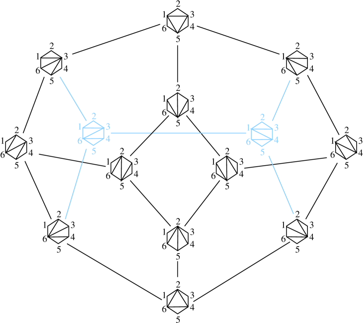
Figure 4. The exchange graph of the cluster algebra of type $A_{3}$, which coincides with the $1$-skeleton of the associahedron.

Exercise 2.16.

Let $T$ be a triangulation of a polygon, and let $T^{\prime}$ be the new triangulation obtained from $T$ by flipping the diagonal $k$. Then the quiver associated to $T^{\prime}$ is the same as the quiver obtained from $Q(T)$ by mutating at $k$: $Q(T^{\prime})=\mu_{k}(Q(T))$.

Proposition 2.17.

If $T_{1}$ and $T_{2}$ are two triangulations of a $d$-gon, then the cluster algebras $\mathcal{A}(T_{1})$ and $\mathcal{A}(T_{2})$ are isomorphic.

Proof.

This follows from Exercise 2.16 and the fact that the flip-graph is connected. ∎

Since the cluster algebra associated to a triangulation of a $d$-gon depends only on $d$, we will refer to this cluster algebra as $\mathcal{A}_{d-3}$. We’ve chosen to index this cluster algebra by $d-3$ because this cluster algebra has rank $d-3$.

2.2.1. The homogeneous coordinate ring of the Grassmannian $Gr_{2,d}$

We now explain how the cluster algebra associated to a $d$-gon can be identified with the coordinate ring $\mathbb{C}[Gr_{2,d}]$ of (the affine cone over) the Grassmannian $Gr_{2,d}$ of $2$-planes in a $d$-dimensional vector space.

Recall that the coordinate ring $\mathbb{C}[Gr_{2,d}]$ is generated by Plücker coordinates $p_{ij}$ for $1\leq i<j\leq d$. The relations among the Plücker coordinates are generated by the three-term Plücker relations: for any $1\leq i<j<k<\ell\leq d$, one has

(2.4) $$p_{ik}p_{j\ell}=p_{ij}p_{k\ell}+p_{i\ell}p_{jk}.$$

To make the connection with cluster algebras, label the vertices of a $d$-gon from $1$ to $d$ in order around the boundary. Then each side and diagonal of the polygon is uniquely identified by the labels of its endpoints. Note that the Plücker coordinates for $Gr_{2,d}$ are in bijection with the set of sides and diagonals of the polygon, see the right of Figure 3.

By noting that the three-term Plücker relations correspond to exchange relations in $\mathcal{A}_{d-3}$, one may verify the following.

Exercise 2.18.

The cluster and coefficient variables of $\mathcal{A}_{d-3}$ are in bijection with the diagonals and sides of the $d$-gon, and the clusters are in bijection with triangulations of the $d$-gon. Moreover the coordinate ring of $Gr_{2,d}$ is isomorphic to the cluster algebra $\mathcal{A}_{d-3}$ associated to the $d$-gon.

Figure 5. A flip in a quadrilateral and the corresponding exchange relation $p_{ik}p_{j\ell}=p_{ij}p_{k\ell}+p_{i\ell}p_{jk}.$

Remark 2.19.

One may generalize this example of the type A cluster algebra in several ways. First, one may replace $Gr_{2,d}$ by an arbitrary Grassmannian, or partial flag variety. It turns out that the coordinate ring $\mathbb{C}[Gr_{k,d}]$ of any Grassmannian has the structure of a cluster algebra [43], and more generally, so does the coordinate ring of any partial flag variety $SL_{m}(\mathbb{C})/P$ [18]. Second, one may generalize this example by replacing the $d$-gon – topologically a disk with $d$ marked points on the boundary – by an orientable Riemann surface $S$ (with or without boundary) together with some marked points $M$ on $S$. One may still consider triangulations of $(S,M)$, and use the combinatorics of these triangulations to define a cluster algebra. This cluster algebra is closely related to the decorated Teichmulller space associated to $(S,M)$. We will take up this theme in Section 3.

2.3. Cluster algebras revisited

We now give a more general definition of cluster algebra, following [16], in which the coefficient variables have their own dynamics. In Section 4 we will see that the dynamics of coefficient variables is closely related to Zamolodchikov’s Y-systems.

To define a cluster algebra $\mathcal{A}$ we first choose a semifield $(\mathbb{P},\oplus,\cdot)$, i.e., an abelian multiplicative group endowed with a binary operation of (auxiliary) addition $\oplus$ which is commutative, associative, and distributive with respect to the multiplication in $\mathbb{P}$. The group ring $\mathbb{Z}\mathbb{P}$ will be used as a ground ring for $\mathcal{A}$. One important choice for $\mathbb{P}$ is the tropical semifield (see Definition 2.20); in this case we say that the corresponding cluster algebra is of geometric type.

Definition 2.20 (Tropical semifield).

Let $\operatorname{Trop}(u_{1},\dots,u_{m})$ be an abelian group, which is freely generated by the $u_{j}$’s, and written multiplicatively. We define $\oplus$ in $\operatorname{Trop}(u_{1},\dots,u_{m})$ by

(2.5) $$\prod_{j}u_{j}^{a_{j}}\oplus\prod_{j}u_{j}^{b_{j}}=\prod_{j}u_{j}^{\min(a_{j},b_{j})}\,,$$

and call $(\operatorname{Trop}(u_{1},\dots,u_{m}),\oplus,\cdot)$ a tropical semifield. Note that the group ring of $\operatorname{Trop}(u_{1},\dots,u_{m})$ is the ring of Laurent polynomials in the variables $u_{j}\,$.

As an ambient field for $\mathcal{A}$, we take a field $\mathcal{F}$ isomorphic to the field of rational functions in $n$ independent variables (here $n$ is the rank of $\mathcal{A}$), with coefficients in $\mathbb{Q}\mathbb{P}$. Note that the definition of $\mathcal{F}$ does not involve the auxiliary addition in $\mathbb{P}$.

Definition 2.21 (Labeled seeds).

A labeled seed in $\mathcal{F}$ is a triple $(\mathbf{x},\mathbf{y},B)$, where

• $\mathbf{x}=(x_{1},\dots,x_{n})$ is an $n$-tuple from $\mathcal{F}$ forming a free generating set over $\mathbb{Q}\mathbb{P}$, that is, $x_{1},\dots,x_{n}$ are algebraically independent over $\mathbb{Q}\mathbb{P}$, and $\mathcal{F}=\mathbb{Q}\mathbb{P}(x_{1},\dots,x_{n})$.

• $\mathbf{y}=(y_{1},\dots,y_{n})$ is an $n$-tuple from $\mathbb{P}$, and

• $B=(b_{ij})$ is an $n\!\times\!n$ integer matrix which is skew-symmetrizable, that is, there exist positive integers $d_{1},\dots,d_{n}$ such that $d_{i}b_{ij}=-d_{j}b_{ij}$.

We refer to $\mathbf{x}$ as the (labeled) cluster of a labeled seed $(\mathbf{x},\mathbf{y},B)$, to the tuple $\mathbf{y}$ as the coefficient tuple, and to the matrix $B$ as the exchange matrix.

We obtain (unlabeled) seeds from labeled seeds by identifying labeled seeds that differ from each other by simultaneous permutations of the components in $\mathbf{x}$ and $\mathbf{y}$, and of the rows and columns of $B$.

In what follows, we use the notation $[x]_{+}=\max(x,0)$.

Definition 2.22 (Seed mutations).

Let $(\mathbf{x},\mathbf{y},B)$ be a labeled seed in $\mathcal{F}$, and let $k\in\{1,\dots,n\}$. The seed mutation $\mu_{k}$ in direction $k$ transforms $(\mathbf{x},\mathbf{y},B)$ into the labeled seed $\mu_{k}(\mathbf{x},\mathbf{y},B)=(\mathbf{x}^{\prime},\mathbf{y}^{\prime},B^{\prime})$ defined as follows:

• The entries of $B^{\prime}=(b^{\prime}_{ij})$ are given by

  (2.6) $$b^{\prime}_{ij}=\begin{cases}-b_{ij}&\text{if $i=k$ or $j=k$;}\\[3.61371pt] b_{ij}+b_{ik}b_{kj}&\text{if $b_{ik}>0$ and $b_{kj}>0$;}\\[3.61371pt] b_{ij}-b_{ik}b_{kj}&\text{if $b_{ik}<0$ and $b_{kj}<0$;}\\[3.61371pt] b_{ij}&\text{otherwise.}\end{cases}$$

• The coefficient tuple $\mathbf{y}^{\prime}=(y_{1}^{\prime},\dots,y_{n}^{\prime})$ is given by

  (2.7) $$y^{\prime}_{j}=\begin{cases}y_{k}^{-1}&\text{if $j=k$};\\[3.61371pt] y_{j}y_{k}^{[b_{kj}]_{+}}(y_{k}\oplus 1)^{-b_{kj}}&\text{if $j\neq k$}.\end{cases}$$

• The cluster $\mathbf{x}^{\prime}=(x_{1}^{\prime},\dots,x_{n}^{\prime})$ is given by $x_{j}^{\prime}=x_{j}$ for $j\neq k$, whereas $x^{\prime}_{k}\in\mathcal{F}$ is determined by the exchange relation

  (2.8) $$x^{\prime}_{k}=\frac{y_{k}\ \prod x_{i}^{[b_{ik}]_{+}}+\ \prod x_{i}^{[-b_{ik}]_{+}}}{(y_{k}\oplus 1)x_{k}}\,.$$

We say that two exchange matrices $B$ and $B^{\prime}$ are mutation-equivalent if one can get from $B$ to $B^{\prime}$ by a sequence of mutations.

If we forget the cluster variables, then we refer to the resulting seeds and operation of mutation as Y-seeds and Y-seed mutation.

Definition 2.23 (Y-seed mutations).

Let $(\mathbf{y},B)$ be a labeled seed in which we have omitted the cluster $\mathbf{x}$, and let $k\in\{1,\dots,n\}$. The Y-seed mutation $\mu_{k}$ in direction $k$ transforms $(\mathbf{y},B)$ into the labeled Y-seed $\mu_{k}(\mathbf{y},B)=(\mathbf{y}^{\prime},B^{\prime})$, where $\mathbf{y}^{\prime}$ and $B^{\prime}$ are as in Definition 2.22.

Definition 2.24 (Patterns).

Consider the $n$-regular tree $\mathbb{T}_{n}$ whose edges are labeled by the numbers $1,\dots,n$, so that the $n$ edges emanating from each vertex receive different labels. A cluster pattern is an assignment of a labeled seed $\Sigma_{t}=(\mathbf{x}_{t},\mathbf{y}_{t},B_{t})$ to every vertex $t\in\mathbb{T}_{n}$, such that the seeds assigned to the endpoints of any edge $t\!\begin{array}[]{c}\scriptstyle{k}\\[-7.22743pt] -\!\!\!-\!\!\!-\\[-7.22743pt] {}\scriptstyle\hfil\end{array}\!t^{\prime}$ are obtained from each other by the seed mutation in direction $k$. The components of $\Sigma_{t}$ are written as:

(2.9) $$\mathbf{x}_{t}=(x_{1;t}\,,\dots,x_{n;t})\,,\quad\mathbf{y}_{t}=(y_{1;t}\,,\dots,y_{n;t})\,,\quad B_{t}=(b^{t}_{ij})\,.$$

One may view a cluster pattern as a discrete dynamical system on an $n$-regular tree. If we ignore the coefficients (i.e. if we set each coefficient tuple equal to $(1,\dots,1)$ and choose a semifield such that $1\oplus 1=1$), then we refer to the evolution of the cluster variables as cluster dynamics. On the other hand, ignoring the cluster variables, we refer to the evolution of the coefficient variables as coefficient dynamics.

Definition 2.25 (Cluster algebra).

Given a cluster pattern, we denote

(2.10) $$\mathcal{X}=\bigcup_{t\in\mathbb{T}_{n}}\mathbf{x}_{t}=\{x_{i,t}\,:\,t\in\mathbb{T}_{n}\,,\ 1\leq i\leq n\}\ ,$$

the union of clusters of all the seeds in the pattern. The elements $x_{i,t}\in\mathcal{X}$ are called cluster variables. The cluster algebra $\mathcal{A}$ associated with a given pattern is the $\mathbb{Z}\mathbb{P}$-subalgebra of the ambient field $\mathcal{F}$ generated by all cluster variables: $\mathcal{A}=\mathbb{Z}\mathbb{P}[\mathcal{X}]$. We denote $\mathcal{A}=\mathcal{A}(\mathbf{x},\mathbf{y},B)$, where $(\mathbf{x},\mathbf{y},B)$ is any seed in the underlying cluster pattern.

We now explain the relationship between Definition 2.11 – the definition of cluster algebra we gave in Section 2.1 – and Definition 2.25. There are two apparent differences between the definitions. First, in Definition 2.11, the dynamics of mutation was encoded by a quiver, while in Definition 2.25, the dynamics of mutation was encoded by a skew-symmetrizable matrix $B$. Clearly if $B$ is not only skew-symmetrizable but also skew-symmetric, then $B$ can be regarded as the signed adjacency matrix of a quiver. In that case mutation of $B$ reduces to the mutation of the corresponding quiver, and the two notions of exchange relation coincide. Second, in Definition 2.11, the coefficient variables are “frozen” and do not mutate, while in Definition 2.25, the coefficient variables $y_{i}$ have a dynamics of their own. It turns out that if in Definition 2.25 the semifield $\mathbb{P}$ is the tropical semifield (and $B$ is skew-symmetric), then Definitions 2.11 and 2.25 are equivalent. This is a consequence of the following exercise.

Exercise 2.26.

Let $\mathbb{P}=\operatorname{Trop}(x_{n+1},\dots,x_{m})$ be the tropical semifield with generators $x_{n+1},\dots,x_{m}$, and consider a cluster algebra as defined in Definition 2.25. Since the coefficients $y_{j;t}$ at the seed $\Sigma_{t}=(\mathbf{x}_{t},\mathbf{y}_{t},B_{t})$ are Laurent monomials in $x_{n+1},\dots,x_{m}$, we may define the integers $b_{ij}^{t}$ for $j\in\{1,\dots,n\}$ and $n<i\leq m$ by

$$y_{j;t}=\prod_{i=n+1}^{m}x_{i}^{b_{ij}^{t}}.$$

This gives a natural way of including the exchange matrix $B_{t}$ as the principal $n\times n$ submatrix into a larger $m\times n$ matrix $\widetilde{B}_{t}=(b_{ij}^{t})$ where $1\leq i\leq m$ and $1\leq j\leq n$, whose matrix elements $b_{ij}^{t}$ with $i>n$ encode the coefficients $y_{j}=y_{j;t}$.

Check that with the above conventions, the exchange relation (2.8) reduces to the exchange relation (2.2), and that the Y-seed mutation rule (2.7) implies that the extended exchange matrix $\widetilde{B}_{t}$ mutates according to (2.1).

2.4. Structural properties of cluster algebras

In this section we will explain various structural properties of cluster algebras. Throughout this section $\mathcal{A}$ will be an arbitrary cluster algebra as defined in Section 2.3.

From the definitions, it is clear that any cluster variable can be expressed as a rational function in the variables of an arbitrary cluster. However, the remarkable Laurent phenomenon, proved in [13, Theorem 3.1], asserts that each such rational function is actually a Laurent polynomial.

Theorem 2.27 (Laurent Phenomenon).

The cluster algebra $\mathcal{A}$ associated with a seed $\Sigma=(\mathbf{x},\mathbf{y},B)$ is contained in the Laurent polynomial ring $\mathbb{Z}\mathbb{P}[\mathbf{x}^{\pm 1}]$, i.e. every element of $\mathcal{A}$ is a Laurent polynomial over $\mathbb{Z}\mathbb{P}$ in the cluster variables from $\mathbf{x}=(x_{1},\dots,x_{n})$.

Let $\mathcal{A}$ be a cluster algebra, $\Sigma$ be a seed, and $x$ be a cluster variable of $\mathcal{A}$. Let $[x]_{\Sigma}^{\mathcal{A}}$ denote the Laurent polynomial which expresses $x$ in terms of the cluster variables from $\Sigma$; it is called the cluster expansion of $x$ in terms of $\Sigma$. The longstanding Positivity Conjecture [13] says that the coefficients that appear in such Laurent polynomials are positive.

Conjecture 2.28 (Positivity Conjecture).

For any cluster algebra $\mathcal{A}$, any seed $\Sigma$, and any cluster variable $x$, the Laurent polynomial $[x]_{\Sigma}^{\mathcal{A}}$ has coefficients which are nonnegative integer linear combinations of elements in $\mathbb{P}$.

While Conjecture 2.28 is open in general, it has been proved in some special cases, see for example [2], [37], [38], [5], [24], [31].

One of Fomin-Zelevinsky’s motivations for introducing cluster algebras was the desire to understand the canonical bases of quantum groups due to Lusztig and Kashiwara [34, 28]. See [19] for some recent results connecting cluster algebras and canonical bases. Some of the conjectures below, including Conjectures 2.30 and 2.32, are motivated in part by the conjectural connection between cluster algebras and canonical bases.

Definition 2.29 (Cluster monomial).

A cluster monomial in a cluster algebra $\mathcal{A}$ is a monomial in cluster variables, all of which belong to the same cluster.

Conjecture 2.30.

Cluster monomials are linearly independent.

The best result to date towards Conjecture 2.30 is the following.

Theorem 2.31.

[3] In a cluster algebra defined by a quiver, the cluster monomials are linearly independent.

The following conjecture has long been a part of the cluster algebra folklore, and it implies both Conjecture 2.28 and Conjecture 2.30.

Conjecture 2.32 (Strong Positivity Conjecture).

Any cluster algebra has an additive basis $\mathbb{B}$ which

• includes the cluster monomials, and

• has nonnegative structure constants, that is, when one writes the product of any two elements in $\mathbb{B}$ in terms of $\mathbb{B}$, the coefficients are positive.

One of the most striking results about cluster algebras is that the classification of the finite type cluster algebras is parallel to the Cartan-Killing classification of complex simple Lie algebras. In particular, finite type cluster algebras are classified by Dynkin diagrams.

Definition 2.33 (Finite type).

We say that a cluster algebra is of finite type if it has finitely many seeds.

It turns out that the classification of finite type cluster algebras is parallel to the Cartan-Killing classification of complex simple Lie algebras [14]. More specifically, define the diagram $\Gamma(B)$ associated to an $n\times n$ exchange matrix $B$ to be a weighted directed graph on nodes $v_{1},\dots,v_{n}$, with $v_{i}$ directed towards $v_{j}$ if and only if $b_{ij}>0$. In that case, we label this edge by $|b_{ij}b_{ji}|.$

Theorem 2.34.

[14, Theorem 1.8] The cluster algebra $\mathcal{A}$ is of finite type if and only if it has a seed $(\mathbf{x},\mathbf{y},B)$ such that $\Gamma(B)$ is an orientation of a finite type Dynkin diagram.

If the conditions of Theorem 2.34 hold, we say that $\mathcal{A}$ is of finite type. And in that case if $\Gamma(B)$ is an orientation of a Dynkin diagram of type $X$ (here $X$ belongs to one of the infinite series $A_{n}$, $B_{n}$, $C_{n}$, $D_{n}$, or to one of the exceptional types $E_{6}$, $E_{7}$, $E_{8}$, $F_{4}$, $G_{2}$), we say that the cluster algebra $\mathcal{A}$ is of type $X$.

We define the exchange graph of a cluster algebra to be the graph whose vertices are the (unlabeled) seeds, and whose edges connect pairs of seeds which are connected by a mutation. When a cluster algebra is of finite type, its exchange graph has a remarkable combinatorial structure.

Theorem 2.35.

[4] Let $\mathcal{A}$ be a cluster algebra of finite type. Then its exchange graph is the $1$-skeleton of a convex polytope.

When $\mathcal{A}$ is a cluster algebra of type $A$, its exchange graph is the $1$-skeleton of a famous polytope called the associahedron, see Figure 4. Therefore the polytopes that arise from finite type cluster algebras as in Theorem 2.35 are called generalized associahedra.

3. Cluster algebras in Teichmüller theory

In this section we will explain how cluster algebras had already appeared implicitly in Teichmüller theory, before the introduction of cluster algebras themselves. In particular, we will associate a cluster algebra to any bordered surface with marked points, following work of Fock-Goncharov [8], Gekhtman-Shapiro-Vainshtein [20], and Fomin-Shapiro-Thurston [11]. This construction provides a natural generalization of the type A cluster algebra from Section 2.2, and realizes the lambda lengths (also called Penner coordinates) on the decorated Teichmüller space associated to a cusped surface, which Penner had defined in 1987 [39]. We will also briefly discuss the Teichmüller space of a surface with oriented geodesic boundary and related spaces of laminations, and how these spaces are related to cluster theory. For more details on the Teichmüller and lamination spaces, see [9].

3.1. Surfaces, arcs, and triangulations

Definition 3.1 (Bordered surface with marked points).

Let $S$ be a connected oriented 2-dimensional Riemann surface with (possibly empty) boundary. Fix a nonempty set $M$ of marked points in the closure of $S$ with at least one marked point on each boundary component. The pair $(S,M)$ is called a bordered surface with marked points. Marked points in the interior of $S$ are called punctures.

For technical reasons we require that $(S,M)$ is not a sphere with one, two or three punctures; a monogon with zero or one puncture; or a bigon or triangle without punctures.

Definition 3.2 (Arcs and boundary segments).

An arc $\gamma$ in $(S,M)$ is a curve in $S$, considered up to isotopy, such that: the endpoints of $\gamma$ are in $M$; $\gamma$ does not cross itself, except that its endpoints may coincide; except for the endpoints, $\gamma$ is disjoint from $M$ and from the boundary of $S$; and $\gamma$ does not cut out an unpunctured monogon or an unpunctured bigon.

A boundary segment is a curve that connects two marked points and lies entirely on the boundary of $S$ without passing through a third marked point.

Let $A(S,M)$ and $B(S,M)$ denote the sets of arcs and boundary segments in $(S,M)$. Note that $A(S,M)$ and $B(S,M)$ are disjoint.

Definition 3.3 (Compatibility of arcs, and triangulations).

We say that arcs $\gamma$ and $\gamma^{\prime}$ are compatible if there exist curves $\alpha$ and $\alpha^{\prime}$ isotopic to $\gamma$ and $\gamma^{\prime}$, such that $\alpha$ and $\alpha^{\prime}$ do not cross. A triangulation is a maximal collection of pairwise compatible arcs (together with all boundary segments). The arcs of a triangulation cut the surface into triangles.

There are two types of triangles: triangles that have three distinct sides, and self-folded triangles that have only two. Note that a self-folded triangle consists of a loop, together with an arc to an enclosed puncture, called a radius, see Figure 6.

Figure 6. Two triangulations of a once-punctured polygon. The triangulation at the right contains a self-folded triangle.

Definition 3.4 (Flips).

A flip of a triangulation $T$ replaces a single arc $\gamma\in T$ by a (unique) arc $\gamma^{\prime}\neq\gamma$ that, together with the remaining arcs in $T$, forms a new triangulation.

In Figure 6, the triangulation at the right is obtained from the triangulation at the left by flipping the arc between the marked points $3$ and $5$. However, a radius inside a self-folded triangle in $T$ cannot be flipped (see e.g. the arc between $1$ and $5$ at the right).

Proposition 3.5.

[22, 23, 36] Any two triangulations of a bordered surface are related by a sequence of flips.

3.2. Decorated Teichmüller space

In this section we assume that the reader is familiar with some basics of hyperbolic geometry.

Definition 3.6 (Teichmüller space).

Let $(S,M)$ be a bordered surface with marked points. The (cusped) Teichmüller space $\mathcal{T}(S,M)$ consists of all complete finite-area hyperbolic metrics with constant curvature $-1$ on $S\setminus M$, with geodesic boundary at $\partial S\setminus M$, considered up to $\operatorname{Diff}_{0}(S,M)$, diffeomorphisms of $S$ fixing $M$ that are homotopic to the identity. (Thus there is a cusp at each point of $M$: points at $M$ “go off to infinity,” while the area remains bounded.)

For a given hyperbolic metric in $\mathcal{T}(S,M)$, each arc can be represented by a unique geodesic. Since there are cusps at the marked points, such a geodesic segment is of infinite length. So if we want to measure the “length” of a geodesic arc between two marked points, we need to renormalize.

To do so, around each cusp $p$ we choose a horocycle, which may be viewed as the set of points at an equal distance from $p$. Although the cusp is infinitely far away from any point in the surface, there is still a well-defined way to compare the distance to $p$ from two different points in the surface. A horocycle can also be characterized as a curve perpendicular to every geodesic to $p$. See Figure 7 for a depiction of some points and horocycles, drawn in the hyperbolic plane.

The notion of horocycle leads to the following definition.

Definition 3.7 (Decorated Teichmüller space).

A point in a decorated Teichmüller space $\widetilde{\mathcal{T}}(S,M)$ is a hyperbolic metric as above together with a collection of horocyles $h_{p}$, one around each cusp corresponding to a marked point $p\in M$.

One may parameterize decorated Teichmüller space using lambda lengths or Penner coordinates, as introduced and developed by Penner [39, 40].

Definition 3.8 (Lambda lengths).

[40] Fix $\sigma\in\widetilde{\mathcal{T}}(S,M)$. Let $\gamma$ be an arc or a boundary segment. Let $\gamma_{\sigma}$ denote the geodesic representative of $\gamma$ (relative to $\sigma$). Let $\ell(\gamma)=\ell_{\sigma}(\gamma)$ be the signed distance along $\gamma_{\sigma}$ between the horocycles at either end of $\gamma$ (positive if the two horocycles do not intersect, and negative if they do). The lambda length $\lambda(\gamma)=\lambda_{\sigma}(\gamma)$ of $\gamma$ is defined by

(3.1) $$\lambda(\gamma)=\exp(\ell(\gamma)/2).$$

Given $\gamma\in A(S,M)\cup B(S,M)$, one may view the lambda length

$$\lambda(\gamma):\sigma\mapsto\lambda_{\sigma}(\gamma)$$

as a function on the decorated Teichmüller space $\widetilde{\mathcal{T}}(S,M)$. Let $n$ denote the number of arcs in a triangulation of $(S,M)$; recall that $c$ denotes the number of marked points on the boundary of $S$. Penner showed that if one fixes a triangulation $T$, then the lambda lengths of the arcs of $T$ and the boundary segments can be used to parameterize $\widetilde{\mathcal{T}}(S,M)$:

Theorem 3.9.

For any triangulation $T$ of $(S,M)$, the map

$$\prod_{\gamma\in T\cup B(S,M)}\lambda(\gamma):\widetilde{\mathcal{T}}(S,M)\to\mathbb{R}_{>0}^{n+c}$$

is a homeomorphism.

Note that the first versions of Theorem 3.9 were due to Penner [39, Theorem 3.1], [40, Theorem 5.10], but the formulation above is from [12, Theorem 7.4].

The following “Ptolemy relation” is an indication that lambda lengths on decorated Teichmüller space are part of a related cluster algebra.

Proposition 3.10.

[39, Proposition 2.6(a)] Let $\alpha,\beta,\gamma,\delta\in A(S,M)\cup B(S,M)$ be arcs or boundary segments (not necessarily distinct) that cut out a quadrilateral in $S$; we assume that the sides of the quadrilateral, listed in cyclic order, are $\alpha,\beta,\gamma,\delta$. Let $\eta$ and $\theta$ be the two diagonals of this quadrilateral. Then the corresponding lambda lengths satisfy the Ptolemy relation

$$\lambda(\eta)\lambda(\theta)=\lambda(\alpha)\lambda(\gamma)+\lambda(\beta)\lambda(\delta).$$

Figure 7. Four points and corresponding horocycles, together with the arcs forming the geodesics between them, drawn in the hyperbolic plane. At the left, all lengths $\ell(\alpha),\dots,\ell(\theta)$ are positive; but at the right, $\ell(\gamma)$ is negative.

3.3. The cluster algebra associated to a surface

To make precise the connection between decorated Teichmüller space and cluster algebras, let us fix a triangulation $T$ of $(S,M)$, and explain how to associate an exchange matrix $B_{T}$ to $T$ [8, 10, 20, 11]. For simplicity we assume that $T$ has no self-folded triangles. It is not hard to see that all of the bordered surfaces we are considering admit a triangulation without self-folded triangles.

Definition 3.11 (Exchange matrices associated to a triangulation).

Let $T$ be a triangulation of $(S,M)$. Let $\tau_{1},\tau_{2},\ldots,\tau_{n}$ be the $n$ arcs of $T$, and $\tau_{n+1},\dots,\tau_{n+c}$ be the $c$ boundary segments of $(S,M)$. We define

$$b_{ij}= \#\{\text{triangles with sides }\tau_{i}\text{ and }\tau_{j},\text{ with }\tau_{j}\text{ following }\tau_{i}\text{ in clockwise order}\}-$$

$$\#\{\text{triangles with sides }\tau_{i}\text{ and }\tau_{j},\text{ with }\tau_{j}\text{ following }\tau_{i}\text{ in counterclockwise order}\}.$$

Then we define the exchange matrix $B_{T}=(b_{ij})_{1\leq i\leq n,1\leq j\leq n}$ and the extended exchange matrix $\widetilde{B}_{T}=(b_{ij})_{1\leq i\leq n+c,1\leq j\leq n}$.

In Figure 7 there is a triangle with sides $\alpha$, $\beta$, and $\eta$, and our convention is that $\beta$ follows $\alpha$ in clockwise order. Note that in order to speak about clockwise order, one must be working with an oriented surface. That is why Definition 3.1 requires $S$ to be oriented.

We leave the following as an exercise for the reader; alternatively, see [11].

Exercise 3.12.

Extend Definition 3.11 to the case that $T$ has self-folded triangles, so that the exchange matrices transform compatibly with mutation.

Remark 3.13.

Note that each entry $b_{ij}$ of the exchange matrix (or extended exchanged matrix) is either $0,\pm 1$, or $\pm 2$, since every arc $\tau$ is in at most two triangles.

Exercise 3.14.

Note that $B_{T}$ is skew-symmetric, and hence can be viewed as the signed adjacency matrix associated to a quiver. Verify that this quiver generalizes the quiver $Q(T)$ from Definition 2.12 associated to a triangulation of a polygon.

The following result is proved by interpreting cluster variables as lambda lengths of arcs, and using the fact that lambda lengths satisfy Ptolemy relations. It also uses the fact that any two triangulations of $(S,M)$ can be connected by a sequence of flips.

Theorem 3.15.

Let $(S,M)$ be a bordered surface and let $T=(\tau_{1},\dots,\tau_{n})$ be a triangulation of $(S,M)$. Let $\mathbf{x}_{T}=(x_{\tau_{1}},\dots,x_{\tau_{n}})$, and let $\mathcal{A}=\mathcal{A}(\mathbf{x}_{T},B_{T})$ be the corresponding cluster algebra. Then we have the following:

• Each arc $\gamma\in A(S,M)$ gives rise to a cluster variable $x_{\gamma}$;

• Each triangulation $T$ of $(S,M)$ gives rise to a seed $\Sigma_{T}=(x_{T},B_{T})$ of $\mathcal{A}$;

• If $T^{\prime}$ is obtained from $T$ by flipping at $\tau_{k}$, then $B_{T^{\prime}}=\mu_{k}(B_{T})$.

It follows that the cluster algebra $\mathcal{A}$ does not depend on the triangulation $T$, but only on $(S,M)$. Therefore we refer to this cluster algebra as $\mathcal{A}(S,M)$.

Remark 3.16.

Theorem 3.15 gives an inclusion of arcs into the set of cluster variables of $\mathcal{A}(S,M)$. This inclusion is a bijection if and only if $(S,M)$ has no punctures. In [11], Fomin-Shapiro-Thurston introduced tagged arcs and tagged triangulations, which generalize arcs and triangulations, and are in bijection with cluster variables and clusters of $\mathcal{A}(S,M)$, see [11, Theorem 7.11]. To each tagged triangulation one may associate an exchange matrix, which as before has all entries equal to $0$, $\pm 1$, or $\pm 2$.

Combining Theorem 3.15 with Theorem 3.9 and Proposition 3.10, we may identify the cluster variable $x_{\gamma}$ with the corresponding lambda length $\lambda(\gamma)$, and therefore view such elements of the cluster algebra $\mathcal{A}$ as functions on $\widetilde{\mathcal{T}}(S,M)$. In particular, when one performs a flip in a triangulation, the lambda lengths associated to the arcs transform according to cluster dynamics.

It is natural to consider whether there is a nice system of coordinates on Teichmüller space $\mathcal{T}(S,M)$ itself (as opposed to its decorated version.) Indeed, if one fixes a point of $\mathcal{T}(S,M)$ and a triangulation $T$ of $(S,M)$, one may represent $T$ by geodesics and lift it to an ideal triangulation of the upper half plane. Note that every arc of the triangulation is the diagonal of a unique quadrilateral. The four points of this quadrilateral have a unique invariant under the action of $PSL_{2}(\mathbb{R})$, the cross-ratio. One may compute the cross-ratio by sending three of the four points to $0$, $-1$, and $\infty$. Then the position $x$ of the fourth point is the cross-ratio. The collection of cross-ratios associated to the arcs in $T$ comprise a system of coordinates on $\mathcal{T}(S,M)$. And when one performs a flip in the triangulation, the coordinates transform according to coefficient dynamics, see [9, Section 4.1].

3.4. Spaces of laminations and their coordinates

Several compactifications of Teichmüller space have been introduced. The most widely used compactification is due to W. Thurston [45, 46]; the points at infinity of this compactification correspond to projective measured laminations.

Informally, a measured lamination on $(S,M)$ is a finite collection of non-self-intersecting and pairwise non-intersecting weighted curves in $S\setminus M$, considered up to homotopy, and modulo a certain equivalence relation. It is not hard to see why such a lamination $L$ might correspond to a limit point of Teichmüller space $\mathcal{T}(S,M)$: given $L$, one may construct a family of metrics on the surface “converging to $L$,” by cutting at each curve in $L$ and inserting a “long neck.” As the necks get longer and longer, the length of an arbitrary curve in the corresponding metric becomes dominated by the number of times that curve crosses $L$. Therefore $L$ represents the limit of this family of metrics.

Interestingly, two versions of the space of laminations on $(S,M)$ – the space of rational bounded measured laminations, and the space of rational unbounded measured laminations – are closely connected to cluster theory. In both cases, one may fix a triangulation $T$ and then use appropriate coordinates to get a parameterization of the space. The appropriate coordinates for the space of rational bounded measured laminations are intersection numbers. Let $T^{\prime}$ be a triangulation obtained from $T$ by performing a flip. It turns out that when one replaces $T$ by $T^{\prime}$, the rule for how intersection numbers change is given by a tropical version of cluster dynamics. On the other hand, the appropriate coordinates for the space of rational unbounded measured laminations are shear coordinates. When one replaces $T$ by $T^{\prime}$, the rule for how shear coordinates change is given by a tropical version of coefficient dynamics. See [9] for more details.

In Table 1, we summarize the properties of the two versions of Teichmüller space, and the two versions of the space of laminations, together with their coordinates.

Space	Coordinates	Coordinate transformations
Decorated Teichmüller space	Lambda lengths	Cluster dynamics
Teichmüller space	Cross-ratios	Coefficient dynamics
Bounded measured laminations	Intersection numbers	Tropical cluster dynamics
Unbounded measured laminations	Shear coordinates	Tropical coefficient dynamics

Table 1. Teichmüller and lamination spaces.

3.5. Applications of Teichmüller theory to cluster theory

The connection between Teichmüller theory and cluster algebras has useful applications to cluster algebras, some of which we discuss below.

As mentioned in Remark 3.16, the combinatorics of (tagged) arcs and (tagged) triangulations gives a concrete way to index cluster variables and clusters in a cluster algebra from a surface. Additionally, the combinatorics of unbounded measured laminations gives a concrete way to encode the coefficient variables for a cluster algebra, whose coefficient system is of geometric type [12]. Recall from Section 2.1 or Exercise 2.26 that the coefficient system is determined by the bottom $m-n$ rows of the initial extended exchange matrix $\widetilde{B}$. However, after one has mutated away from the initial cluster, one would like an explicit way to read off the resulting coefficient variables (short of performing the corresponding sequence of mutations). In [12], the authors demonstrated that one may encode the initial extended exchange matrix by a triangulation together with a lamination, and that one may compute the coefficient variables (even after mutating away from the initial cluster) by using shear coordinates.

Note that for a general cluster algebra, there is no explicit way to index cluster variables or clusters, or to encode the coefficients. A cluster variable is simply a rational function of the initial cluster variables that is obtained after some arbitrary and arbitrarily long sequence of mutations. Having a concrete index set for the cluster variables and clusters, as in [11, Theorem 7.11], is a powerful tool. Indeed, this was a key ingredient in [37], which proved the Positivity Conjecture for all cluster algebras from surfaces.

The connection between Teichmüller theory and cluster algebras from surfaces has also led to important structural results for such cluster algebras. We say that a cluster algebra has polynomial growth if the number of distinct seeds which can be obtained from a fixed initial seed by at most $n$ mutations is bounded from above by a polynomial function of $n$. A cluster algebra has exponential growth if the number of such seeds is bounded from below by an exponentially growing function of $n$. In [11], Fomin-Shapiro-Thurston classified the cluster algebras from surfaces according to their growth: there are six infinite families which have polynomial growth, and all others have exponential growth.

Another structural result relates to the classification of mutation-finite cluster algebras. We say that a matrix $B$ (and the corresponding cluster algebra) is mutation-finite (or is of finite mutation type) if its mutation equivalence class is finite, i.e. only finitely many matrices can be obtained from $B$ by repeated matrix mutations. Felikson-Shapiro-Tumarkin gave a classification of all skew-symmetric mutation-finite cluster algebras in [7]. They showed that these cluster algebras are the union of the following classes of cluster algebras:

• Rank 2 cluster algebras;

• Cluster algebras from surfaces;

• One of 11 exceptional types.

Note that the above classification may be extended to all mutation-finite cluster algebras (not necessarily skew-symmetric), using cluster algebras from orbifolds [6].

Exercise 3.17.

Show that any cluster algebra from a surface is mutation-finite. Hint: use Remark 3.16.

4. Cluster algebras and the Zamolodchikov periodicity conjecture

The thermodynamic Bethe ansatz is a tool for understanding certain conformal field theories. In a paper from 1991 [48], the physicist Al. B. Zamolodchikov studied the thermodynamic Bethe ansatz equations for ADE-related diagonal scattering theories. He showed that if one has a solution to these equations, it should also be a solution of a set of functional relations called a Y-system. Furthermore, he remarked that based on numerical tests, the solutions to the Y-system appeared to be periodic. This phenomenon is called the Zamolodchikov periodicity conjecture, and has important consequences for the corresponding field theory. Although this conjecture arose in mathematical physics, we will see that it can be reformulated and proved using the framework of cluster algebras.

Note that Zamolodchikov initially stated his conjecture for the Y-system of a simply-laced Dynkin diagram. The notion of Y-system and the periodicity conjecture were subsequently generalized by Ravanini-Valleriani-Tateo [42], Kuniba-Nakanishi [32], Kuniba-Nakanishi-Suzuki [33], Fomin-Zelevinsky [15], etc. We will first present Zamolodchikov’s periodicity conjecture for Dynkin diagrams $\Delta$ (not necessarily simply-laced), and then present its extension to pairs $(\Delta,\Delta^{\prime})$ of Dynkin diagrams. Note that the latter conjecture reduces to the former in the case that $\Delta^{\prime}=A_{1}$. The conjecture was proved for $(A_{n},A_{1})$ by Frenkel-Szenes [17] and Gliozzi-Tateo [21]; for $(\Delta,A_{1})$ (where $\Delta$ is an arbitrary Dynkin diagram) by Fomin-Zelevinsky [15]; and for $(A_{n},A_{m})$ by Volkov [47] and independently by Szenes [44]. Finally in 2008, Keller proved the conjecture in the general case [29, 30], using cluster algebras and their additive categorification via triangulated categories. Another proof was subsequently given by Inoue-Iyama-Keller-Kuniba-Nakanishi [25, 26].

In Sections 4.1 and 4.2 we will state the periodicity conjecture for Dynkin diagrams and pairs of Dynkin diagrams, respectively, and explain how the conjectures may be formulated in terms of cluster algebras. In Section 4.3 we will discuss how techniques from the theory of cluster algebras were used to prove the conjectures.

4.1. Zamolodchikov’s Periodicity Conjecture for Dynkin diagrams

Let $\Delta$ be a Dynkin diagram with vertex set $I$. Let $A$ denote the incidence matrix of $\Delta$, i.e. if $C$ is the Cartan matrix of $\Delta$ and $J$ the identity matrix of the same size, then $A=2J-C$. Let $h$ denote the Coxeter number of $\Delta$, see Table 2.

$\Delta$	$A_{n}$	$B_{n}$	$C_{n}$	$D_{n}$	$E_{6}$	$E_{7}$	$E_{8}$	$F_{4}$	$G_{2}$
$h$	$n+1$	$2n$	$2n$	$2n-2$	$12$	$18$	$30$	$12$	$6$

Table 2. Coxeter numbers.

Theorem 4.1 (Zamolodchikov’s periodicity conjecture).

Consider the recurrence relation

(4.1) $$Y_{i}(t+1)Y_{i}(t-1)=\prod_{j\in I}(Y_{j}(t)+1)^{a_{ij}},\quad t\in\mathbb{Z}.$$

All solutions to this system are periodic in $t$ with period dividing $2(h+2)$, i.e. $Y_{i}(t+2(h+2))=Y_{i}(t)$ for all $i$ and $t$.

The system of equations in (4.1) is called a Y-system.

Note that any Dynkin diagram is a tree, and hence its set $I$ of vertices is the disjoint union of two sets $I_{+}$ and $I_{-}$ such that there is no edge between any two vertices of $I_{+}$ nor between any two vertices of $I_{-}$. Define $\epsilon(i)$ to be $1$ or $-1$ based on whether $i\in I_{+}$ or $i\in I_{-}$. Let $\mathbb{Q}(u)$ be the field of rational functions in the variables $u_{i}$ for $i\in I$. For $\epsilon=\pm 1$, define an automorphism $\tau_{\epsilon}$ by setting

$$\tau_{\epsilon}(u_{i})=\begin{cases}u_{i}\prod_{j\in I}(u_{j}+1)^{a_{ij}}&\text{ if $\epsilon(i)=\epsilon$}\\ u_{i}^{-1}&\text{ otherwise.}\end{cases}$$

One may reformulate Zamolodchikov’s periodicity conjecture in terms of $\tau_{\epsilon}$, as we will see below in Lemma 4.4. First note that the variables $Y_{i}(k)$ on the left-hand side of (4.1) have a fixed “parity” $\epsilon(i)(-1)^{k}$. Therefore the Y-system decomposes into two independent systems, an even one and an odd one, and it suffices to prove periodicity for one of them. Without loss of generality, we may therefore assume that

$$Y_{i}(k+1)=Y_{i}(k)^{-1}\text{ whenever }\epsilon(i)=(-1)^{k}.$$

If we combine this assumption with (4.1), we obtain

(4.2) $$Y_{i}(k+1)=\begin{cases}Y_{i}(k){\prod_{j\in I}(Y_{j}(k)+1)^{a_{ij}}}&\text{ if $\epsilon(i)=(-1)^{k+1}$}\\ Y_{i}(k)^{-1}&\text{ if $\epsilon(i)=(-1)^{k}$.}\end{cases}$$

Example 4.2.

Let $\Delta$ be the Dynkin diagram of type $A_{2}$, on nodes $1$ and $2$, where $I_{-}=\{1\}$ and $I_{+}=\{2\}$. The incidence matrix of the Dynkin diagram is

$$A=\begin{pmatrix}0&1\\ 1&0\end{pmatrix}.$$

If we set $Y_{1}(0)=u_{1}$, $Y_{2}(0)=u_{2}$, then the recurrence for $Y_{i}(k)$ in (4.2) yields:

$$Y_{1}(0) =u_{1}\,, Y_{2}(0) =u_{2}$$

$$Y_{1}(1) =u_{1}^{-1}\,, Y_{2}(1) =u_{2}(1+u_{1})$$

$$Y_{1}(2) =\frac{1+u_{2}+u_{1}u_{2}}{u_{1}}\,, Y_{2}(2) =\frac{1}{u_{2}(1+u_{1})}$$

$$Y_{1}(3) =\frac{u_{1}}{1+u_{2}+u_{1}u_{2}}\,, Y_{2}(3) =\frac{1+u_{2}}{u_{1}u_{2}}$$

$$Y_{1}(4) =u_{2}^{-1}\,, Y_{2}(4) =\frac{u_{1}u_{2}}{1+u_{2}}$$

$$Y_{1}(5) ={u_{2}}\,, Y_{2}(5) =u_{1}.$$

By symmetry, it’s clear that $Y_{1}(10)=u_{1}$ and $Y_{2}(10)=u_{2}$ and this system has period $10=2(3+2)$, as predicted by Theorem 4.1.

The following lemma follows easily from induction and the definition of $\tau_{\epsilon}$.

Lemma 4.3.

Set $Y_{i}(0)=u_{i}$ for $i\in I$. Then for all $k\in\mathbb{Z}_{\geq 0}$ and $i\in I$, we have $Y_{i}(k)=(\tau_{-}\tau_{+}\dots\tau_{\pm})(u_{i})$, where the number of factors $\tau_{+}$ and $\tau_{-}$ equals $k$.

Let us define an automorphism of $\mathbb{Q}(u)$ by

(4.3) $$\phi=\tau_{-}\tau_{+}.$$

Then we have the following.

Lemma 4.4.

The Y-system from (4.1) is periodic with period dividing $2(h+2)$ if and only if $\phi$ has finite order dividing $h+2$.

To connect Zamolodchikov’s conjecture to cluster algebras, let us revisit the notion of Y-seed mutation from Definition 2.23. We will assume that $B$ is skew-symmetric, and hence can be encoded by a finite quiver $Q$ without loops or $2$-cycles. Let $(\mathbb{P},\oplus,\cdot)$ be $\mathbb{Q}$ with the usual operations of addition and multiplication. Then $\mu_{k}(\mathbf{y},Q)=(\mathbf{y}^{\prime},Q^{\prime})$, where

$$y_{j}^{\prime}=\begin{cases}y_{k}^{-1}&\text{ if $j=k$}\\ y_{j}(1+y_{k})^{m}&\text{ if there are $m\geq 0$ arrows $j\to k$}\\ y_{j}(1+y_{k}^{-1})^{-m}&\text{ if there are $m\geq 0$ arrows $k\to j$.}\end{cases}$$

Comparing the formula for Y-seed mutation with the definition of the automorphisms $\tau_{\epsilon}$ suggests a connection, which we make precise in Exercise 4.6. First we will define a restricted $Y$-pattern.

Definition 4.5 (Restricted $Y$-pattern).

Let $(\mathbb{P},\oplus,\cdot)$ be $\mathbb{Q}$ with the usual operations of addition and multiplication. Let $Q$ denote a finite quiver without loops or $2$-cycles with vertex set $\{1,\dots,n\}$, let $\mathbf{y}=(y_{1},\dots,y_{n})$ and let $(\mathbf{y},Q)$ be the corresponding Y-seed. Let $\mathbf{v}$ be a sequence of vertices $v_{1},\dots,v_{N}$ of $Q$, with the property that the composed mutation

$$\mu_{\mathbf{v}}=\mu_{v_{N}}\dots\mu_{v_{2}}\mu_{v_{1}}$$

transforms $Q$ into itself. Then clearly the same holds for the same sequence in reverse $\mu_{\mathbf{v}}^{-1}$. We define the restricted $Y$-pattern associated with $Q$ and $\mu_{\mathbf{v}}$ to be the sequence of Y-seeds obtained from the initial Y-seed $(\mathbf{y},Q)$ be applying all integer powers of $\mu_{\mathbf{v}}$.

Exercise 4.6.

Let $\Delta$ be a simply-laced Dynkin diagram with $n$ vertices, and vertex set $I=I_{+}\cup I_{-}$ as above. Let $Q$ denote the unique “bipartite” orientation of $\Delta$ such that each vertex in $I_{+}$ is a source and each vertex in $I_{-}$ is a sink.

1. Then the composed mutation $\mu_{+}=\prod_{i\in I_{-}}\mu_{i}$ is well-defined, in other words, any sequence of mutations on the vertices in $I_{-}$ yields the same result. Similarly $\mu_{-}=\prod_{i\in I_{+}}\mu_{i}$ is well-defined.

2. The composed mutation $\mu_{-}\mu_{+}$ transforms $Q$ into itself. Similarly for $\mu_{+}\mu_{-}$.

3. The automorphism $\tau_{-}\tau_{+}$ has finite order $m$ if and only if the restricted $Y$-pattern associated with $Q$ and $\mu_{-}\mu_{+}$ is periodic with period $m$.

Combining Exercise 4.6 with Lemma 4.3, we see that Zamolodchikov’s periodicity conjecture is equivalent to verifying the periodicity of the restricted $Y$-pattern from Exercise 4.6 (3). See Figure 8 for an example of Y-seed mutation on the Dynkin diagram of type $A_{2}$. Compare the labeled Y-seeds here with Example 4.2.

Figure 8. Y-seeds and Y-seed mutations in type $A_{2}$.

4.2. The periodicity conjecture for pairs of Dynkin diagrams

In this section we let $\Delta$ and $\Delta^{\prime}$ be Dynkin diagrams, with vertex sets $I$ and $I^{\prime}$, and incidence matrices $A$ and $A^{\prime}$.

Theorem 4.7 (The periodicity conjecture for pairs of Dynkin diagrams).

Consider the recurrence relation

(4.4) $$Y_{i,i^{\prime}}(t+1)Y_{i,i^{\prime}}(t-1)=\frac{\prod_{j\in I}(Y_{j,i^{\prime}}(t)+1)^{a_{ij}}}{\prod_{j^{\prime}\in I^{\prime}}(Y_{i,j^{\prime}}(t)^{-1}+1)^{a^{\prime}_{i^{\prime},j^{\prime}}}},\quad t\in\mathbb{Z}.$$

All solutions to this system are periodic in $t$ with period dividing $2(h+h^{\prime})$.

Note that if $\Delta^{\prime}$ is of type $A_{1}$, then Theorem 4.7 reduces to Theorem 4.1.

Just as we saw for Theorem 4.1, it is possible to reformulate Theorem 4.7 in terms of certain automorphisms. Write $I=I_{+}\cup I_{-}$ and $I^{\prime}=I^{\prime}_{+}\cup I^{\prime}_{-}$ as before. For a vertex $(i,i^{\prime})$ of the product $I\times I^{\prime}$, define $\epsilon(i,i^{\prime})$ to be $1$ or $-1$ based on whether $(i,i^{\prime})$ lies in $(I_{+}\times I^{\prime}_{+})\cup(I_{-}\times I^{\prime}_{-})$ or not. Let $\mathbb{Q}(u)$ be the field of rational functions in the variables $u_{ii^{\prime}}$ for $i\in I$ and $i^{\prime}\in I^{\prime}$, and define an automorphism of $\mathbb{Q}(u)$ by

(4.5) $$\phi=\tau_{-}\tau_{+},\text{ where }$$

$$\tau_{\epsilon}(u_{ii^{\prime}})=\begin{cases}u_{ii^{\prime}}\prod_{j\in I}(u_{ji^{\prime}}+1)^{a_{ij}}\prod_{j^{\prime}\in I^{\prime}}(u_{ij^{\prime}}^{-1}+1)^{-a^{\prime}_{i^{\prime}j^{\prime}}}&\text{ if $\epsilon(i,i^{\prime})=\epsilon$}\\ u_{ii^{\prime}}^{-1}&\text{ otherwise.}\end{cases}$$

As before, we may assume that $Y_{i,i^{\prime}}(k+1)=Y_{i,i^{\prime}}(k)^{-1}$ whenever $\epsilon(i,i^{\prime})=(-1)^{k}.$ One may then reformulate the periodicity conjecture as follows.

Lemma 4.8.

The periodicity conjecture for pairs of Dynkin diagrams holds if and only if $\phi$ has finite order dividing $h+h^{\prime}$.

Now let us explain how to relate the periodicity conjecture for pairs of Dynkin diagrams to cluster algebras (more specifically, restricted $Y$-patterns). We first need to define some operations on quivers.

Let $Q$ and $Q^{\prime}$ be two finite quivers on vertex sets $I$ and $I^{\prime}$ which are bipartite, i.e. each vertex is a source or a sink. The tensor product $Q\otimes Q^{\prime}$ is the quiver on vertex set $I\times I^{\prime}$, where the number of arrows from a vertex $(i,i^{\prime})$ to a vertex $(j,j^{\prime})$

1. is zero if $i\neq j$ and $i^{\prime}\neq j^{\prime}$;

2. equals the number of arrows from $j$ to $j^{\prime}$ if $i=i^{\prime}$;

3. equals the number of arrows from $i$ to $i^{\prime}$ if $j=j^{\prime}$.

The square product $Q\square Q^{\prime}$ is the quiver obtained from $Q\otimes Q^{\prime}$ by reversing all arrows in the full subquivers of the form $\{i\}\times Q^{\prime}$ and $Q\times\{i^{\prime}\}$, where $i$ is a sink of $Q$ and $i^{\prime}$ a source of $Q^{\prime}$. See Figure 9 for an example of the square product of the following quivers.

$$\vec{A}_{4} :\lx@xy@svg{\hbox{\raise 0.0pt\hbox{\kern 5.5pt\hbox{\ignorespaces\ignorespaces\ignorespaces\hbox{\vtop{\kern 0.0pt\offinterlineskip\halign{\entry@#!@&&\entry@@#!@\cr&&&\crcr}}}\ignorespaces{\hbox{\kern-5.5pt\raise 0.0pt\hbox{\hbox{\kern 0.0pt\raise 0.0pt\hbox{\hbox{\kern 3.0pt\raise 0.0pt\hbox{$\textstyle{1}$}}}}}}}{\hbox{\kern 29.5pt\raise 0.0pt\hbox{\hbox{\kern 0.0pt\raise 0.0pt\hbox{\hbox{\kern 3.0pt\raise 0.0pt\hbox{$\textstyle{2\ignorespaces\ignorespaces\ignorespaces\ignorespaces\ignorespaces\ignorespaces\ignorespaces\ignorespaces}$}}}}}}}\ignorespaces\ignorespaces\ignorespaces\ignorespaces{}{\hbox{\lx@xy@droprule}}\ignorespaces{\hbox{\kern 5.50002pt\raise 0.0pt\hbox{\hbox{\kern 0.0pt\raise 0.0pt\hbox{\lx@xy@tip{1}\lx@xy@tip{-1}}}}}}{\hbox{\lx@xy@droprule}}{\hbox{\lx@xy@droprule}}\ignorespaces\ignorespaces\ignorespaces\ignorespaces{}{\hbox{\lx@xy@droprule}}\ignorespaces{\hbox{\kern 64.5pt\raise 0.0pt\hbox{\hbox{\kern 0.0pt\raise 0.0pt\hbox{\lx@xy@tip{1}\lx@xy@tip{-1}}}}}}{\hbox{\lx@xy@droprule}}{\hbox{\lx@xy@droprule}}{\hbox{\kern 64.5pt\raise 0.0pt\hbox{\hbox{\kern 0.0pt\raise 0.0pt\hbox{\hbox{\kern 3.0pt\raise 0.0pt\hbox{$\textstyle{3}$}}}}}}}{\hbox{\kern 99.5pt\raise 0.0pt\hbox{\hbox{\kern 0.0pt\raise 0.0pt\hbox{\hbox{\kern 3.0pt\raise 0.0pt\hbox{$\textstyle{4\ignorespaces\ignorespaces\ignorespaces\ignorespaces}$}}}}}}}\ignorespaces\ignorespaces\ignorespaces\ignorespaces{}{\hbox{\lx@xy@droprule}}\ignorespaces{\hbox{\kern 75.50002pt\raise 0.0pt\hbox{\hbox{\kern 0.0pt\raise 0.0pt\hbox{\lx@xy@tip{1}\lx@xy@tip{-1}}}}}}{\hbox{\lx@xy@droprule}}{\hbox{\lx@xy@droprule}}\ignorespaces}}}}\ignorespaces\>,\; \textstyle{1} \textstyle{2\ignorespaces\ignorespaces\ignorespaces\ignorespaces\ignorespaces\ignorespaces\ignorespaces\ignorespaces} \textstyle{3} \textstyle{4\ignorespaces\ignorespaces\ignorespaces\ignorespaces} \textstyle{1} \textstyle{2\ignorespaces\ignorespaces\ignorespaces\ignorespaces\ignorespaces\ignorespaces\ignorespaces\ignorespaces} \textstyle{3} \textstyle{4\ignorespaces\ignorespaces\ignorespaces\ignorespaces}$$

$$\vec{D}_{5} :\raisebox{21.33955pt}{\lx@xy@svg{\hbox{\raise 0.0pt\hbox{\kern 5.5pt\hbox{\ignorespaces\ignorespaces\ignorespaces\hbox{\vtop{\kern 0.0pt\offinterlineskip\halign{\entry@#!@&&\entry@@#!@\cr&&&\\&&&\\&&&\crcr}}}\ignorespaces{\hbox{\kern-3.0pt\raise 0.0pt\hbox{\hbox{\kern 0.0pt\raise 0.0pt\hbox{\hbox{\kern 3.0pt\raise 0.0pt\hbox{$\textstyle{}$}}}}}}}{\hbox{\kern 32.0pt\raise 0.0pt\hbox{\hbox{\kern 0.0pt\raise 0.0pt\hbox{\hbox{\kern 3.0pt\raise 0.0pt\hbox{$\textstyle{}$}}}}}}}{\hbox{\kern 67.0pt\raise 0.0pt\hbox{\hbox{\kern 0.0pt\raise 0.0pt\hbox{\hbox{\kern 3.0pt\raise 0.0pt\hbox{$\textstyle{}$}}}}}}}{\hbox{\kern 100.8889pt\raise 0.0pt\hbox{\hbox{\kern 0.0pt\raise 0.0pt\hbox{\hbox{\kern 3.0pt\raise 0.0pt\hbox{$\textstyle{4\ignorespaces\ignorespaces\ignorespaces\ignorespaces}$}}}}}}}\ignorespaces\ignorespaces\ignorespaces{}\ignorespaces\ignorespaces{\hbox{\lx@xy@drawline@}}\ignorespaces{\hbox{\kern 75.50002pt\raise-15.39563pt\hbox{\hbox{\kern 0.0pt\raise 0.0pt\hbox{\lx@xy@tip{1}\lx@xy@tip{-1}}}}}}\ignorespaces\ignorespaces{\hbox{\lx@xy@drawline@}}\ignorespaces{\hbox{\lx@xy@drawline@}}{\hbox{\kern-5.5pt\raise-18.13489pt\hbox{\hbox{\kern 0.0pt\raise 0.0pt\hbox{\hbox{\kern 3.0pt\raise 0.0pt\hbox{$\textstyle{1}$}}}}}}}{\hbox{\kern 29.5pt\raise-18.13489pt\hbox{\hbox{\kern 0.0pt\raise 0.0pt\hbox{\hbox{\kern 3.0pt\raise 0.0pt\hbox{$\textstyle{2\ignorespaces\ignorespaces\ignorespaces\ignorespaces\ignorespaces\ignorespaces\ignorespaces\ignorespaces}$}}}}}}}\ignorespaces\ignorespaces\ignorespaces\ignorespaces{}{\hbox{\lx@xy@droprule}}\ignorespaces{\hbox{\kern 5.50002pt\raise-18.13489pt\hbox{\hbox{\kern 0.0pt\raise 0.0pt\hbox{\lx@xy@tip{1}\lx@xy@tip{-1}}}}}}{\hbox{\lx@xy@droprule}}{\hbox{\lx@xy@droprule}}\ignorespaces\ignorespaces\ignorespaces\ignorespaces{}{\hbox{\lx@xy@droprule}}\ignorespaces{\hbox{\kern 64.5pt\raise-18.13489pt\hbox{\hbox{\kern 0.0pt\raise 0.0pt\hbox{\lx@xy@tip{1}\lx@xy@tip{-1}}}}}}{\hbox{\lx@xy@droprule}}{\hbox{\lx@xy@droprule}}{\hbox{\kern 64.5pt\raise-18.13489pt\hbox{\hbox{\kern 0.0pt\raise 0.0pt\hbox{\hbox{\kern 3.0pt\raise 0.0pt\hbox{$\textstyle{3}$}}}}}}}{\hbox{\kern 103.3889pt\raise-18.13489pt\hbox{\hbox{\kern 0.0pt\raise 0.0pt\hbox{\hbox{\kern 3.0pt\raise 0.0pt\hbox{$\textstyle{}$}}}}}}}{\hbox{\kern-3.0pt\raise-36.26978pt\hbox{\hbox{\kern 0.0pt\raise 0.0pt\hbox{\hbox{\kern 3.0pt\raise 0.0pt\hbox{$\textstyle{}$}}}}}}}{\hbox{\kern 32.0pt\raise-36.26978pt\hbox{\hbox{\kern 0.0pt\raise 0.0pt\hbox{\hbox{\kern 3.0pt\raise 0.0pt\hbox{$\textstyle{}$}}}}}}}{\hbox{\kern 67.0pt\raise-36.26978pt\hbox{\hbox{\kern 0.0pt\raise 0.0pt\hbox{\hbox{\kern 3.0pt\raise 0.0pt\hbox{$\textstyle{}$}}}}}}}{\hbox{\kern 99.5pt\raise-36.26978pt\hbox{\hbox{\kern 0.0pt\raise 0.0pt\hbox{\hbox{\kern 3.0pt\raise 0.0pt\hbox{$\textstyle{5.\ignorespaces\ignorespaces\ignorespaces\ignorespaces}$}}}}}}}\ignorespaces\ignorespaces\ignorespaces{}\ignorespaces\ignorespaces{\hbox{\lx@xy@drawline@}}\ignorespaces{\hbox{\kern 75.50002pt\raise-20.86877pt\hbox{\hbox{\kern 0.0pt\raise 0.0pt\hbox{\lx@xy@tip{1}\lx@xy@tip{-1}}}}}}\ignorespaces\ignorespaces{\hbox{\lx@xy@drawline@}}\ignorespaces{\hbox{\lx@xy@drawline@}}\ignorespaces}}}}\ignorespaces} \textstyle{4\ignorespaces\ignorespaces\ignorespaces\ignorespaces} \textstyle{1} \textstyle{2\ignorespaces\ignorespaces\ignorespaces\ignorespaces\ignorespaces\ignorespaces\ignorespaces\ignorespaces} \textstyle{3} \textstyle{5.\ignorespaces\ignorespaces\ignorespaces\ignorespaces} \textstyle{4\ignorespaces\ignorespaces\ignorespaces\ignorespaces} \textstyle{1} \textstyle{2\ignorespaces\ignorespaces\ignorespaces\ignorespaces\ignorespaces\ignorespaces\ignorespaces\ignorespaces} \textstyle{3} \textstyle{5.\ignorespaces\ignorespaces\ignorespaces\ignorespaces}$$

Figure 9. The quiver $\vec{A}_{4}\square\vec{D}_{5}$

Exercise 4.9.

Let $\Delta$ and $\Delta^{\prime}$ be simply-laced Dynkin diagrams with vertex sets $I$ and $I^{\prime}$. We write $I=I_{+}\cup I_{-}$ and $I^{\prime}=I^{\prime}_{+}\cup I^{\prime}_{-}$ as usual, and choose the corresponding bipartite orientations $Q$ and $Q^{\prime}$ of $\Delta$ and $\Delta^{\prime}$ so that each vertex in $I_{+}$ or $I^{\prime}_{+}$ is a source and each vertex in $I_{-}$ or $I^{\prime}_{-}$ is a sink.

1. Given two elements $\sigma,\sigma^{\prime}$ of $\{+,-\}$, the following composed mutation

   $$\mu_{\sigma,\sigma^{\prime}}=\prod_{i\in I_{\sigma},\ i^{\prime}\in I^{\prime}_{\sigma^{\prime}}}\mu_{(i,i^{\prime})}$$

   of $Q\square Q^{\prime}$ is well-defined, that is, the order in the product does not matter.

2. The composition $\mu_{\square}=\mu_{-,-}\ \mu_{+,+}\ \mu_{-,+}\ \mu_{+,-}$ transforms $Q$ into itself.

3. The automorphism $\phi$ has finite order $m$ if and only if the restricted Y-seed associated with $Q\square Q^{\prime}$ and $\mu_{\square}$ is periodic with period $m$.

Combining Exercise 4.9 with Lemma 4.8, we have the following:

Lemma 4.10.

The periodicity conjecture holds for $\Delta$ and $\Delta^{\prime}$ if and only if the restricted Y-seed associated with $Q\square Q^{\prime}$ and $\mu_{\square}$ is periodic with period dividing $h+h^{\prime}$.

4.3. On the proofs of the periodicity conjecture

In this section we discuss how techniques from the theory of cluster algebras were used to prove Theorems 4.1 and 4.7.

First note that the proofs of Theorem 4.1 and Theorem 4.7 can be reduced to the case that the Dynkin diagrams are simply-laced, using standard “folding” arguments. Second, as illustrated in Exercises 4.6 and 4.9, the periodicity conjecture for simply-laced Dynkin diagrams may be reformulated in terms of cluster algebras. Specifically, the conjecture is equivalent to verifying the periodicity of certain restricted $Y$-patterns.

Fomin-Zelevinsky’s proof of Theorem 4.1 used ideas which are now fundamental to the structure theory of finite type cluster algebras, including a bijection between cluster variables and “almost-positive” roots of the corresponding root system. They showed that this bijection, together with a “tropical” version of Theorem 4.1, implies Theorem 4.1. Moreover, they gave an explicit solution to each Y-system, in terms of certain Fibonacci polynomials. The Fibonacci polynomials are (up to a twist) special cases of F-polynomials, which in turn are important objects in cluster algebras, and control the dynamics of both cluster and coefficient variables [16]. Note however that the Fomin-Zelevinsky proof does not apply to Theorem 4.7, because the cluster algebras associated with products $Q\square Q^{\prime}$ are not in general of finite type.

Keller’s proof of Theorem 4.7 used the additive categorification (via triangulated categories) of cluster algebras. To give some background on categorification, in 2003, Marsh-Reineke-Zelevinsky [35] discovered that when $\Delta$ is a simply-laced Dynkin diagram, there is a close resemblance between the combinatorics of the cluster variables and those of the tilting modules in the category of representations of the quiver; this initiated the theory of additive categorification of cluster algebras. In this theory, one seeks to construct module or triangulated categories associated to quivers so as to obtain a correspondence between rigid objects of the categories and the cluster monomials in the cluster algebras. The required correspondence sends direct sum decompositions of rigid objects to factorizations of the associated cluster monomials. One may then hope to use the rich structure of these categories to prove results on cluster algebras which seem beyond the scope of purely combinatorial methods.

Recall from Section 4.2 that the periodicity conjecture for pairs of Dynkin diagrams is equivalent to the periodicity of the automorphism $\phi$ from (4.5), which in turn is equivalent to the periodicity of a restricted $Y$-pattern associated to $Q\square Q^{\prime}$. Keller’s central construction from [30] was a triangulated 2-Calabi-Yau category $\mathcal{C}$ with a cluster-tilting object $T$, whose endoquiver (quiver of its endomorphism algebra) is closely related to $Q\square Q^{\prime}$; the category $\mathcal{C}$ is a generalized cluster category in the sense of Amiot [1]. Since $\mathcal{C}$ is 2-Calabi-Yau, results of Iyama-Yoshino [27] imply that there is a well-defined mutation operation for the cluster-tilting objects. Keller defined the Zamolodchikov transformation $Za:\mathcal{C}\to\mathcal{C}$, which one may think of as a categorification of the automorphism $\phi$, and proved that $Za$ is periodic of period $h+h^{\prime}$. By “decategorification,” it follows that $\phi$ is periodic of period $h+h^{\prime}$, and hence the periodicity conjecture for pairs of Dynkin diagrams is true.

The Inoue-Iyama-Keller-Kuniba-Nakanishi proof of Theorem 4.7 also used categorification, in particular the work of Plamondon [41]. Moreover, just as in the case of the Fomin-Zelevinsky proof of Theorem 4.7, one crucial ingredient in their proof was a “tropical” version of Theorem 4.7.

References

- [1] Claire Amiot, Cluster categories for algebras of global dimension 2 and quivers with potential, Ann. Inst. Fourier (Grenoble) 59 (2009), no. 6, 2525–2590. MR 2640929 (2011c:16026)
- [2] Philippe Caldero and Markus Reineke, On the quiver Grassmannian in the acyclic case, J. Pure Appl. Algebra 212 (2008), no. 11, 2369–2380. MR 2440252 (2009f:14102)
- [3] Giovanni Cerulli Irelli, Bernhard Keller, Daniel Labardini-Fragoso, and Pierre-Guy Plamondon, Linear independence of cluster monomials for skew-symmetric cluster algebras, ArXiv Mathematics e-prints (2012), arXiv:1203.1307.
- [4] Frédéric Chapoton, Sergey Fomin, and Andrei Zelevinsky, Polytopal realizations of generalized associahedra, Canad. Math. Bull. 45 (2002), no. 4, 537–566, Dedicated to Robert V. Moody. MR 1941227 (2003j:52014)
- [5] Philippe Di Francesco and Rinat Kedem, -systems, heaps, paths and cluster positivity, Comm. Math. Phys. 293 (2010), no. 3, 727–802. MR 2566162 (2010m:13032)
- [6] Anna Felikson, Michael Shapiro, and Pavel Tumarkin, Cluster algebras of finite mutation type via unfoldings, Int. Math. Res. Not. IMRN (2012), no. 8, 1768–1804. MR 2920830
- [7] by same author, Skew-symmetric cluster algebras of finite mutation type, J. Eur. Math. Soc. (2012), no. 14, 1135–1180.
- [8] Vladimir Fock and Alexander Goncharov, Moduli spaces of local systems and higher Teichmüller theory, Publ. Math. Inst. Hautes Études Sci. (2006), no. 103, 1–211. MR 2233852 (2009k:32011)
- [9] by same author, Dual Teichmüller and lamination spaces, Handbook of Teichmüller theory. Vol. I, IRMA Lect. Math. Theor. Phys., vol. 11, Eur. Math. Soc., Zürich, 2007, pp. 647–684. MR 2349682 (2008k:32033)
- [10] by same author, Cluster ensembles, quantization and the dilogarithm, Ann. Sci. Éc. Norm. Supér. (4) 42 (2009), no. 6, 865–930. MR 2567745 (2011f:53202)
- [11] Sergey Fomin, Michael Shapiro, and Dylan Thurston, Cluster algebras and triangulated surfaces. I. Cluster complexes, Acta Math. 201 (2008), no. 1, 83–146. MR 2448067 (2010b:57032)
- [12] Sergey Fomin and Dylan Thurston, Cluster algebras and triangulated surfaces. part ii: Lambda lengths, ArXiv Mathematics e-prints (2012), arXiv:1210.5569.
- [13] Sergey Fomin and Andrei Zelevinsky, Cluster algebras. I. Foundations, J. Amer. Math. Soc. 15 (2002), no. 2, 497–529 (electronic). MR 1887642 (2003f:16050)
- [14] by same author, Cluster algebras. II. Finite type classification, Invent. Math. 154 (2003), no. 1, 63–121. MR 2004457 (2004m:17011)
- [15] by same author, -systems and generalized associahedra, Ann. of Math. (2) 158 (2003), no. 3, 977–1018. MR 2031858 (2004m:17010)
- [16] by same author, Cluster algebras. IV. Coefficients, Compos. Math. 143 (2007), no. 1, 112–164. MR 2295199 (2008d:16049)
- [17] Edward Frenkel and András Szenes, Thermodynamic Bethe ansatz and dilogarithm identities. I, Math. Res. Lett. 2 (1995), no. 6, 677–693. MR 1362962 (97a:11182)
- [18] Christof Geiss, Bernard Leclerc, and Jan Schröer, Partial flag varieties and preprojective algebras, Ann. Inst. Fourier (Grenoble) 58 (2008), no. 3, 825–876. MR 2427512 (2009f:14104)
- [19] by same author, Preprojective algebras and cluster algebras, Trends in representation theory of algebras and related topics, EMS Ser. Congr. Rep., Eur. Math. Soc., Zürich, 2008, pp. 253–283. MR 2484728 (2009m:16024)
- [20] Michael Gekhtman, Michael Shapiro, and Alek Vainshtein, Cluster algebras and Weil-Petersson forms, Duke Math. J. 127 (2005), no. 2, 291–311. MR 2130414 (2006d:53103)
- [21] Ferdinando Gliozzi and Roberto Tateo, Thermodynamic Bethe ansatz and three-fold triangulations, Internat. J. Modern Phys. A 11 (1996), no. 22, 4051–4064. MR 1403679 (97e:82014)
- [22] John Harer, The virtual cohomological dimension of the mapping class group of an orientable surface, Invent. Math. 84 (1986), no. 1, 157–176. MR 830043 (87c:32030)
- [23] Allen Hatcher, On triangulations of surfaces, Topology Appl. 40 (1991), no. 2, 189–194. MR 1123262 (92f:57020)
- [24] David Hernandez and Bernard Leclerc, Cluster algebras and quantum affine algebras, Duke Math. J. 154 (2010), no. 2, 265–341. MR 2682185 (2011g:17027)
- [25] Rei Inoue, Osama Iyama, Bernhard Keller, Atsuo Kuniba, and Tomoki Nakanishi, Periodicities of t and y-systems, dilogarithm identities, and cluster algebras i: Type ., ArXiv Mathematics e-prints (2010), arXiv:1001.1880, to appear in Publ. RIMS.
- [26] by same author, Periodicities of t and y-systems, dilogarithm identities, and cluster algebras ii: Types , , and ., ArXiv Mathematics e-prints (2010), arXiv:1001.1881, to appear in Publ. RIMS.
- [27] Osamu Iyama and Yuji Yoshino, Mutation in triangulated categories and rigid Cohen-Macaulay modules, Invent. Math. 172 (2008), no. 1, 117–168. MR 2385669 (2008k:16028)
- [28] Masaki Kashiwara, On crystal bases of the -analogue of universal enveloping algebras, Duke Math. J. 63 (1991), no. 2, 465–516. MR 1115118 (93b:17045)
- [29] Bernhard Keller, Cluster algebras, quiver representations and triangulated categories, Triangulated categories, London Math. Soc. Lecture Note Ser., vol. 375, Cambridge Univ. Press, Cambridge, 2010, pp. 76–160. MR 2681708 (2011h:13033)
- [30] by same author, The periodicity conjecture for pairs of dynkin diagrams, Ann. Math. 177 (2013).
- [31] Yoshiyuki Kimura and Fan Qin, Graded quiver varieties, quantum cluster algebras, and dual canonical basis, ArXiv Mathematics e-prints (2012), arXiv:1205.2066.
- [32] Atsuo Kuniba and Tomoki Nakanishi, Spectra in conformal field theories from the Rogers dilogarithm, Modern Phys. Lett. A 7 (1992), no. 37, 3487–3494. MR 1192727 (94c:81185)
- [33] Atsuo Kuniba, Tomoki Nakanishi, and Junji Suzuki, Functional relations in solvable lattice models. I. Functional relations and representation theory, Internat. J. Modern Phys. A 9 (1994), no. 30, 5215–5266. MR 1304818 (96h:82003)
- [34] George Lusztig, Canonical bases arising from quantized enveloping algebras, J. Amer. Math. Soc. 3 (1990), no. 2, 447–498. MR 1035415 (90m:17023)
- [35] Robert Marsh, Markus Reineke, and Andrei Zelevinsky, Generalized associahedra via quiver representations, Trans. Amer. Math. Soc. 355 (2003), no. 10, 4171–4186. MR 1990581 (2004g:52014)
- [36] Lee Mosher, Tiling the projective foliation space of a punctured surface, Trans. Amer. Math. Soc. 306 (1988), no. 1, 1–70. MR 927683 (89f:57014)
- [37] Gregg Musiker, Ralf Schiffler, and Lauren Williams, Positivity for cluster algebras from surfaces, Adv. Math. 227 (2011), no. 6, 2241–2308. MR 2807089 (2012f:13052)
- [38] Hiraku Nakajima, Quiver varieties and cluster algebras, Kyoto J. Math. 51 (2011), no. 1, 71–126. MR 2784748 (2012f:13053)
- [39] Robert Penner, The decorated Teichmüller space of punctured surfaces, Comm. Math. Phys. 113 (1987), no. 2, 299–339. MR 919235 (89h:32044)
- [40] by same author, Decorated Teichmüller theory of bordered surfaces, Comm. Anal. Geom. 12 (2004), no. 4, 793–820. MR 2104076 (2006a:32018)
- [41] Pierre-Guy Plamondon, Cluster algebras via cluster categories with infinite-dimensional morphism spaces, Compos. Math. 147 (2011), no. 6, 1921–1934. MR 2862067
- [42] Francesco Ravanini, Angelo Valleriani, and Roberto Tateo, Dynkin TBAs, Internat. J. Modern Phys. A 8 (1993), no. 10, 1707–1727. MR 1216231 (94h:81149)
- [43] Joshua Scott, Grassmannians and cluster algebras, Proc. London Math. Soc. (3) 92 (2006), no. 2, 345–380. MR 2205721 (2007e:14078)
- [44] András Szenes, Periodicity of Y-systems and flat connections, Lett. Math. Phys. 89 (2009), no. 3, 217–230. MR 2551180 (2011b:81116)
- [45] William Thurston, On the geometry and dynamics of diffeomorphisms of surfaces, Bull. Amer. Math. Soc. (N.S.) 19 (1988), no. 2, 417–431. MR 956596 (89k:57023)
- [46] William P. Thurston, The geometry and topology of three-manifolds, Princeton University notes, 1980.
- [47] Alexandre Yu. Volkov, On the periodicity conjecture for -systems, Comm. Math. Phys. 276 (2007), no. 2, 509–517. MR 2346398 (2008m:17021)
- [48] Al. B. Zamolodchikov, On the thermodynamic Bethe ansatz equations for reflectionless scattering theories, Phys. Lett. B 253 (1991), no. 3-4, 391–394. MR 1092210 (92a:81196)