Rotating Unruh-DeWitt Detector in Minkowski Vacuum

Abstract

Response of a circularly rotating Unrh-DeWitt detector to the Minkowski vacuum is investigated. What the detector observes depends on the surface (three volume) to define it by the Hamiltonian. Detectors in the past literature were defined on a surface of a constant Minkowski time, and this is the reason why rotating detectors investigated so far resister particles. No particle is detected by a detector defined by the Hamiltonian on a surface normal to the detector’s orbit, in agreement with the global analysis of vacua. A detector with drift motion superposed on the linear acceleration is also examined, to find the same effect.

I Introduction

Thermalization of a vacuum due to acceleration has been first suggested by Fulling Fulling (1973). Unruh Unruh (1976) and DeWitt DeWitt (1979) have shown that particles with Planckian distribution are actually observed by an accelerated detector in an inertial vacuum (Minkowski vacuum); such a detector is called Unruh-DeWitt detector. After that, numerous papers has been published on this topic to this date (see Takagi (1986); Fulling (2005); Crispino et al. (2008) and references therein). Compared to the well established effect of linear acceleration, the particle detection due to acceleration of rotational motion is still controversial.

Letaw and Pfautsch Letaw and Pfautsch (1981) investigated vacua correspond to various Killing flows in a flat spacetime. They have categorized Killing flows into six classes, and examined the vacuum in each class. Their conclusion is that there are only two inequivalent vacua in a flat spacetime, which they called Minkowski vacuum and Fulling vacuum. The vacuum with the Killing flow of circular rotation is the Minkowski vacuum, which means an observer in rotational motion does not see particles in a Minkowski vacuum. However, analysis using Unruh-DeWitt detector indicates that a rotating detector will resister particles Letaw (1981); Kim et al. (1987) (see also Bell and Leinaas (1983, 1987)).

Davies et al. Davies et al. (1996) found that the existence of a static limit is necessary for the particle detection in a rotating orbit. They have shown that a detector is not excited in the Minkowski vacuum confined in a boundary inside the light cylinder. From this result they suggested the possibility of detector excitation by negative energy. It was Korsbakken and Leinaas Korsbakken and Leinaas (2004) (referred as Paper 1 hereafter) who revealed the actual process of a rotating detector to observe particles; they found the detector is excited by the emission of negative energy quanta.

It was argued in Paper 1 that some wave modes can have negative generalized energy when the flow has a static limit. Here let us use more specific words “Killing energy” for what termed “generalized energy” in Paper 1; it is the energy-momentum along the Killing flow in interest. Two specific Killing flows are investigated in detail in Paper 1: one corresponds to the spatial circular rotation and the other is the flow with drift motion superposed on linear acceleration. The excitation of detector due to the absorption of negative Killing energy was found in both cases.

The present paper is stimulated by the results in Paper 1 and explore the response of accelerating detectors. Our point is that the detector’s response depends on the choice of surface (three volume) to define it, and the detector excitation by negative Killing energy does not occur when we choose the surface appropriately.

The Unruh-DeWitt detector is a hypothetical monopole interacting with the field at one volumeless point. The orbit of the detector is externally given, and its internal energy is the energy measured in the frame comoving with the orbit; it becomes Killing energy when the orbit is along the Killing flow. The detector’s interaction is represented by a small interaction term added to the Hamiltonian of the whole system. In general, a Hamiltonian is defined by the integration of energy-momentum tensor over a surface of a constant time. Therefore, what a detector observes is the Killing energy integrated over the surface of Hamiltonian.

The Hamiltonian used in Paper 1 is on a surface of a constant Minkowski time, which is not normal to the detector’s orbit. The measured Killing energy becomes a combination of energy and momentum integrated over the surface of constant Minkowski time. This can be negative for waves with large negative momentum, and the detector is excited by the emission of such waves.

In contrast, the Killing energy is always positive when integrated over a surface normal to the Killing flow, just like the pressure (three dimensional momentum flow) is always positive. Therefore, a detector does not perceive negative Killing energy when we define it on the normal surface.

These two results do not contradict; two detectors observes different physical quantities which do not have to agree. A similar situation takes place for the acceleration superposed on the drift motion.

In the present paper we first investigate why and how the negative Killing energy modes can exit as a result of the surface choice. As we will see, the negative Killing energy occurs when a wave with phase phase speed slower than the detector crosses the surface oblique to the Killing flow.

Though the wave phase speed is usually faster than the speed of light for planar waves, it can be locally slower in the cylindrical modes for the rotational vacuum as in our case. However, it is not intuitively easy to understand the underlying mechanism with the cylindrical modes expressed with Bessel functions. Therefore, we firstly mimic the slower phase speed using hypothetical planar waves with imaginary mass in Section II. The detector is moving with inertial motion there. This is fake but not entirely unrealistic; we can clarify the mechanism of negative energy mode with it.

Then we move on to the accelerating detectors with realistic models. The response of a rotating detector to the Minkowski vacuum is examined in Section III; we find the detector will not be excited with an appropriate choice of surface. In Section IV another similar motion of detector, motion with drift superposed in acceleration namely, is investigated. Again a properly defined detector has no excitation due to the negative Killing energy; it detects only the particles with Planckian distribution of the ordinary Unruh effect with Doppler shift. Section V is for brief concluding remarks.

II Negative Killing Energy Mode

Here in this section we examine how the negative Killing energy modes occur with a simple and somewhat unrealistic model. To begin with, let us clarify the definition of Killing energy. Let $\zeta_{\mu}$ be the unit vector in the direction of a Killing flow and $T_{\nu}^{\mu}$ be the energy-momentum tensor. What we call Killing energy in the present paper is the energy-momentum along the Killing flow; its flux $j_{\nu}$ is defined as

$$j_{\nu}=\zeta_{\mu}T_{\nu}^{\mu}\,.$$ (1)

The gross Killing energy is obtained by integrating the above flux over a specific surface.

In the following we examine the Killing energy of a real valued two dimensional field with wave equation

$$\phi_{,tt}-\phi_{,xx}-m^{2}\phi=0\,$$ (2)

where we write $\partial\phi/\partial t=\phi_{,t}$, etc., in shorthand. We use the unit system of $c=\hbar=1$ (speed of light = Planck constant = unity) throughout the present paper.

Suppose a hypothetical monopole detector with internal degree of freedom $\mu$ is coupled with the above scalar field $\phi$ by a small coupling constant $c$; the detector is moving along a fixed trajectory $(t,x)=(T(\tau),X(\tau))$, where $\tau$ is the detector’s proper time. The total Hamiltonian of the system is given as

$$H(t)=\int_{t=\textnormal{const}}\left[h_{\phi}+c\left(\frac{dT}{d\tau}\right)^{-1}{\mu}(\tau)\phi(t,x)\delta(x-X)\right]dx+\left(\frac{dT}{d\tau}\right)^{-1}H_{\mu}(\tau(t))$$ (3)

where $h_{\phi}=\frac{1}{2}(\phi_{,t}^{2}+\phi_{,x}^{2}+m^{2}\phi^{2})$ is the Hamiltonian density of the field and $H_{\mu}(\tau)$ is the internal Hamiltonian of the detector, which is independent of the proper time $\tau$. The time evolution of the detector’s internal dynamics is along its propertied $\tau$, which can be inversely written as a function of $t$; $\tau$ and $X$ in the above expression should be understood as $\tau=\tau(t)$ and $X=X(\tau(t))$. The factor $(dT/d\tau)^{-1}$ in the coupling term comes from the same reason, i.e., the interaction takes place along the detector’s proper time $\tau$, while the Hamiltonian is defined along the Minkowski time $t$. It should be noted that the Hamiltonian is defined by the integration over a Cauchy surface of $t=\textnormal{constant}$ which depends on the choice of $(t,x)$ coordinates.

The total Hamiltonian $H(t)$ is time dependent since $X$ depends on time $t$. This means $\partial H/\partial t\neq 0$. On the other hand, the Killing energy is a conserved quantity since the detector moves along the Killing flow. It is conserved locally due to the Noether’s theorem, so its integration over any Cauchy surface is also conserved. Thus we can write

$$\frac{\partial}{\partial t}\int_{t=\textnormal{const}}dx[\zeta_{t}(t,x)h_{\phi}-\zeta_{x}(t,x)p_{\phi}]=\frac{\partial}{\partial\tau}H_{\mu}\,,$$ (4)

where $p_{\phi}=\phi_{,t}\phi_{,x}$ is the momentum flux across the surface of constant $t$. We neglected in the above expression the interaction energy, which vanishes by long time average. The above expression means what the detector measures is the Killing energy integrated over a surface of constant $t$.

Now let us suppose the wave field is in the vacuum and the detector is in the state with lowest energy $E_{0}$; note that the detector’s energy $E$, i.e., the eigenvalue of $H_{\mu}$, is the energy in the detector’s frame since the time evolution with $H_{\mu}$ is determined by the proper time. The detector moves along the Killing flow, thus $E$ is the Killing energy. The state vector of the total system is decomposed as

$$\left|E,\Psi\right\rangle=\left|E_{0}\right\rangle\left|0\right\rangle\,.$$ (5)

The transition by the coupling occurs only for $\left|0\right\rangle\rightarrow\left|1_{k}\right\rangle$ ($1_{k}$ denotes the state with one particle in mode $k$) when the coupling constant $c$ is small enough (see, e.g., DeWitt (2003)):

$$A(E,1;E_{0},0) =ic\left\langle E,1_{k}\right|\int_{-\infty}^{\infty}dt\,\int dx\,\left(\frac{dT}{d\tau}\right)^{-1}\mu(\tau)\phi(t,x)\delta(x-X)\left|E_{0},0\right\rangle$$

$$=ic\left\langle E,1_{k}\right|\int_{-\infty}^{\infty}d\tau\,\mu(\tau)\phi(T(\tau),X(\tau))\left|E_{0},0\right\rangle$$

$$=ic\left\langle E\right|\mu(0)\left|E_{0}\right\rangle\int_{-\infty}^{\infty}d\tau\,e^{i\Delta E\tau}\left\langle 1_{k}\right|\phi(T(\tau),X(\tau))\left|0\right\rangle\,,$$ (6)

In the past literature, the transition amplitude $|A|^{2}$ expressed with the Wightman function is often used to reach the same conclusion. However, we use the above expression because emission/absorption of quanta is more transparent in this form; one can obtain the same result with the Wightman function.

The field can be expanded as

$$\phi=\left(a_{k}^{+}e^{-i\omega t}+a_{k}^{-}e^{i\omega t}\right)\,e^{ikx}\,,$$ (7)

where $\omega>0$ and $a_{k}^{+}$ [$a_{k}^{-}$] are the annihilation [creation] operators for the particles in mode $k$. This definition of annihilation and creation operators is based on the Hamiltonian on the surface of constant $t$, therefore, the detector’s excitation calculated by these operators is in response to the Killing energy integrated over that surface as in (4).

Since the terms with annihilation operator $a_{k}^{+}$ vanishes for the vacuum state $|0\rangle$, the transition coefficient in (6) reduces to

$$\left\langle 1_{k}\right|\phi(T(\tau),X(\tau))\left|0\right\rangle=\exp i(\omega T(\tau)+kX(\tau))\,.$$ (8)

Suppose the detector is moving with a constant velocity $(\zeta_{0t},\zeta_{0x})$, i.e., $(T,X)=(\zeta_{0t}\tau,\zeta_{0x}\tau)$. Then we have

$$\int_{-\infty}^{\infty}d\tau\,e^{i\Delta E\tau}\left\langle 1_{k}\right|\phi(T(\tau),X(\tau))\left|0\right\rangle=\delta(\Delta E+\zeta_{0t}\omega+\zeta_{0x}k)$$ (9)

The above expression vanishes for ordinary plane waves since $\omega>|k|$ and the detector’s speed must be less than unity (=speed of light). Nevertheless, it can survive for mode functions with Bessel (or Macdonald) functions, for which $\omega$ can be smaller than $|k|$ locally, as we will see in the following sections.

However, calculations with Bessel functions in a four dimensional space is complicated and not easy to understand what is happening intuitively. Therefore in this section we artificially assume the mass $m$ is imaginary, i.e., $m^{2}<0$ so that $\omega<|k|$. Although this is somewhat unrealistic, it can demonstrate how a detector is excited by negative Killing-energy.

When $\omega<|k|$ the argument of the $\delta$ function in (9) can be non-zero for a large $k$. This means the detector is excited by the emission of negative Killing energy since the term in (8) is the result of creation operators.

In contrast, such negative Killing energy emission does not occur when we perform the same calculation in the detector’s rest frame. Let us introduce a new frame $\Sigma^{\prime}$ which is moving with a velocity $(u_{t},u_{x})=(\zeta_{0t},\zeta_{0x})$ relative to the original frame (let’s call the original frame $\Sigma$); the coordinates in the frame $\Sigma^{\prime}$ becomes

$$t^{\prime}=\zeta_{0t}t-\zeta_{0x}x\,,\;\;x^{\prime}=\zeta_{0t}x-\zeta_{0x}t$$ (10)

The trajectory of the detector is $(T^{\prime}(\tau),X^{\prime}(\tau))=(t^{\prime},0)$. When we do the same calculation as above, (9) becomes

$$\int_{-\infty}^{\infty}d\tau\,e^{i\Delta E\tau}\left\langle 1_{k}\right|\phi(T^{\prime}(\tau),X^{\prime}(\tau))\left|0\right\rangle=\delta(\Delta E+\omega^{\prime})\,,$$ (11)

where $\omega^{\prime}=|\zeta_{0t}\omega+\zeta_{0x}k|$ is the wave frequency of the creation operator in $\Sigma^{\prime}$. The above expression is always zero since $\omega^{\prime}>0$.

This discrepancy occurs because the the energy-momentum tensor is a flux density and its sign depends on the flow direction across the surface. This situation is illustrated in Figure 1. Two dashed lines indicate the constant time surface in $\Sigma$ and $\Sigma^{\prime}$ respectively, and the hollow arrow is the phase speed of the negative Killing energy mode in $\Sigma$. The energy-momentum carried by this wave crosses the constant time surfaces of $\Sigma$ and $\Sigma^{\prime}$ from the opposite side, and the flux has opposite sign correspondingly.

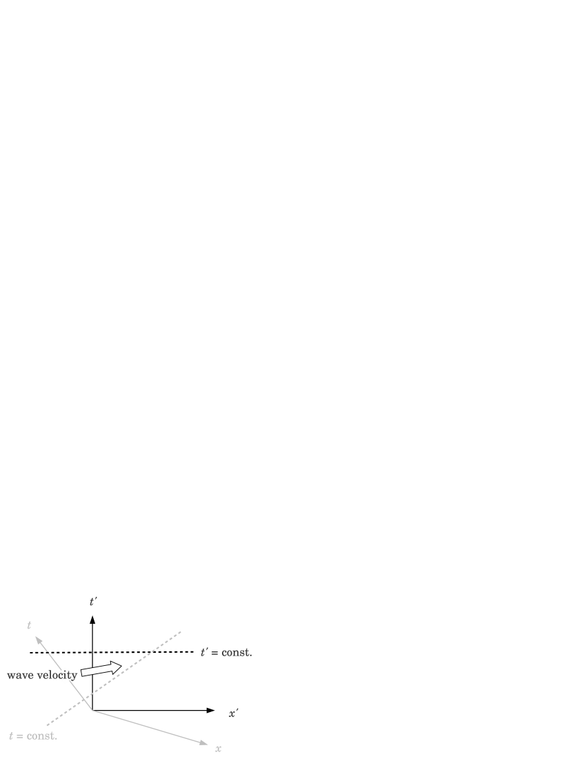
Figure 1: The wave direction crossing the surfaces of constant time. Dashed lines are the time constant surfaces of $\Sigma$ (constant $t$) and $\Sigma^{\prime}$ (constant $t^{\prime}$) respectively. In $\Sigma^{\prime}$ the wave crosses the surface in the increasing $t^{\prime}$ direction, which is decreasing $t$ in $\Sigma$.

From the above consideration, we understand the negative Killing energy in $\Sigma$ becomes positive with the same absolute value in $\Sigma^{\prime}$. Therefore, if we wish to express the Killing energy in $\Sigma^{\prime}$ with the parameters defined on $\Sigma$, straightforward Lorentz transform gives wrong sign. We can obtain the correct answer by replacing $\zeta_{0t}\omega+\zeta_{0x}k$ with $|\zeta_{0t}\omega+\zeta_{0x}k|$.

III Rotating Detector

In this section we examine the response of a rotating detector. Without loss of generality we can express the detector’s orbit using the proper time $\tau$ as

$$(T(\tau),R(\tau),\Theta(\tau),Z(\tau))=(\gamma\tau,r_{0},\gamma\Omega\tau,0)$$ (12)

in the cylindrical coordinates $(t,r,\theta,z)$; the radial distance $r_{0}$ and the angular velocity $\Omega$ are constants, and $\gamma=1/\sqrt{1-\Omega^{2}r_{0}^{2}}$. The detector cannot move faster than the speed of light, thus $1>\Omega r_{0}$.

The massless Klein-Goldon equation in the cylindrical coordinates may be written as

$$\frac{\partial^{2}}{\partial t^{2}}\phi-\left(\frac{1}{r^{2}}\frac{\partial}{\partial r}r\frac{\partial}{\partial r}+\frac{1}{r^{2}}\frac{\partial^{2}}{\partial\theta^{2}}+\frac{\partial^{2}}{\partial z^{2}}\right)\phi=0\,.$$ (13)

The mode functions to the above wave equation is

$$\psi_{hmk}^{\pm}=\frac{J_{m}(hr)}{\sqrt{8\omega\pi^{2}}}\,\exp-i(\pm\omega-m\theta-kz)\,,$$ (14)

where $J_{m}$ is a Bessel function of order $m$ and $\omega=|h|>0$.

The unit vector in the Killing flow direction is expressed as $(\zeta_{t},\zeta_{r},\zeta_{\theta},\zeta_{z})=(\gamma,0,\gamma\Omega r_{0,}0)$. Then the Killing energy of the mode function across the surface of constant $t$ (let us call this surface $S$) becomes

$$E_{S}=\zeta_{t}T_{t}^{t}-\zeta_{\theta}T_{t}^{\theta}=\gamma(\omega+m\Omega)J_{m}(hr_{0})^{2}\,,$$ (15)

at the detector’s orbit. This can be negative for large negative $m\Omega$, which may seem peculiar because it means the local frequency is smaller than the wave number. Suppose we introduce WKB-like approximation in a small region around $(r,\theta)\sim(r_{0},\theta_{0})$ as

$$\psi_{p}^{+}\propto\exp-i(\omega t-k_{r}(r_{0})(r-r_{0})-k_{\theta}r_{0}(\theta-\theta_{0})-k_{z}z)\,,$$ (16)

The above expression is not quantitative approximation, but just a rough sketch to illustrate what is happening. The negative $E_{S}$ means $\omega(r_{0})<|k_{\theta}|$ which is not true for ordinary planar waves since $\omega=\sqrt{k_{r}^{2}+k_{\theta}^{2}+k_{z}^{2}}$. In this case, however, it can be true because the Bessel function $J_{m}(hr)$ exponentially damps in $hr\ll 1$ for large $m$. Then $k_{r}(r_{0})$ in the above approximation becomes imaginary to make $\omega$ smaller than $|k_{\theta}|$. This situation is well mimicked by the imaginary mass we introduced in the previous section, and the details we examined there are also valid here.

On the other hand, the Killing energy across the surface normal to the Killing flow (denoted by $S^{\prime}$) is

$$E_{S^{\prime}}=\zeta_{t}T_{t}^{t}\zeta^{t}-\zeta_{\theta}T_{t}^{\theta}\zeta^{t}-\zeta_{t}T_{\theta}^{t}\zeta^{\theta}+\zeta_{\theta}T_{\theta}^{\theta}\zeta^{\theta}=\gamma^{2}\omega^{-1}(\omega+m\Omega)^{2}J_{m}(hr_{0})^{2}\,,$$ (17)

which is always positive. Note that the above Killing energy density is the one per unit volume. However, energy-momentum of a wave as a physical entity should be a density per wave length because the wave length changes due to the Lorentz transform. The Killing energy density per wave length can be obtained by multiplying the above expression by a factor $\omega\gamma^{-1}/(\omega+m\Omega)$, which yields the energy density $\gamma|\omega+m\Omega|J_{m}^{2}$ in consistent with the result in the previous section.

Now we define the detector in the same way as (3) on $S$. The coefficient for the transition from the Minkowski state to the one particle state is evaluated as as

$$A(E,1_{hmk};E_{0},0_{M}) = ic\left\langle E,1_{hmk}\right|\int_{-\infty}^{\infty}d\tau\,m(\tau)\phi(T(\tau),X_{i}(\tau))\left|E_{0},0\right\rangle$$

$$= ic\left\langle E\right|m(0)\left|E_{0}\right\rangle\int_{-\infty}^{\infty}d\tau\,e^{i\Delta E\tau}\left\langle 1_{k_{hmk}}\right|\phi(T(\tau),X_{i}(\tau))\left|0\right\rangle\,,$$ (18)

where $\Delta E=E-E_{0}$ and $X_{i}(\tau)=(R(\tau),\Theta(\tau),Z(\tau))$ denotes the detector’s spatial position.

We expand the field $\phi$ with the mode functions in (14) as

$$\phi=\sum_{hmk}(a_{hmk}^{+}\psi_{hmk}^{+}+a_{hmk}^{-}\psi_{hmk}^{-})\,.$$ (19)

Mode expansion of the above expression is based on the Hamiltonian on $S$, therefore, the flux of Killing energy calculated with this expansion is the one across the surface $S$ as in the previous section.

The terms with annihilation operators vanish for the transition of $\left|0\right\rangle\rightarrow\left|1_{hmk}\right\rangle$, thus we have

$$\int_{-\infty}^{\infty}d\tau\,e^{i\Delta E\tau} \left\langle 1_{hmk}\right|\phi(T(\tau),X_{i}(\tau)\left|0\right\rangle$$

$$= \frac{J_{m}(hr_{0})}{\sqrt{8\omega\pi^{2}}}\,\int_{-\infty}^{\infty}d\tau\,e^{i\Delta E\tau}\,\exp(i\gamma(\omega+m\Omega)\tau)$$ (20)

$$= \frac{J_{m}(hr_{0})}{\sqrt{8\omega\pi^{2}}}\delta(\Delta E+\gamma(\omega+m\Omega))\,.$$

This means the excitation of the detector takes place when $\omega+m\Omega$ is negative; the rotating detector observes particles due to the emission of negative Killing energy. The amplitude of the above coefficient is small because the Bessel function becomes exponentially small within the static limit when $\omega<|m\Omega|$.

This excitation by negative Killing energy does not occur when we choose the surface $S^{\prime}$ to define the detector as we discussed in the previous section. Let us introduce new coordinates $(s,\varphi,r,z)$ as

$$t=s-r^{2}\Omega\varphi\,,~{}\theta=\varphi+\Omega s\,.$$ (21)

with $r$ and $z$ unchanged. The surface $S^{\prime}$ is specified by a constant $s$, which is normal to the $s$ axis.

The mode functions then become

$$\psi_{hm^{\prime}k}^{\prime\pm}=\frac{1}{\sqrt{8\omega\pi^{2}}}\,e^{\mp\omega^{\prime}s}J_{m}(hr)\,e^{im^{\prime}\varphi}e^{ikz}\,.$$ (22)

where $\omega^{\prime}=|\omega-m\Omega|>0$. The filed can be expanded with these mode functions as

$$\phi=\sum_{hmk}(a_{hm^{\prime}k}^{\prime+}\psi_{hm^{\prime}k}^{\prime+}+a_{hm^{\prime}k}^{\prime-}\psi_{hm^{\prime}k}^{\prime-})\,.$$ (23)

Since $\varphi$ is constant along the orbit, the same calculation as in (20) yields

$$\int_{-\infty}^{\infty}d\tau\,e^{i\Delta E\tau} \left\langle 1_{hmk}\right|\phi(T(\tau),X_{i}(\tau)\left|0\right\rangle$$

$$= \frac{J_{m}(hr_{0})}{\sqrt{8\omega\pi^{2}}}\delta(\Delta E+\gamma\omega^{\prime})\,$$ (24)

The above expression vanishes since the argument of the $\delta$ function is always positive, which means no excitation of the detector.

IV Accelerating Detector with Drift

Another class of vacua was investigated in Paper 1. The Killing flow $K^{\mu}$ to define it is expressed in rectangular coordinates $(t,x,y,z)$ as

$$(K^{t},K^{x},K^{y},K^{z})\propto(\Gamma x,\Gamma t,1,0)\,,$$ (25)

which is a flow accelerating in the $xt$ plane superposed with a constant drift in the $y$ direction. This flow becomes spacelike when $\Gamma\xi<1$ and therefore, the surface of $\Gamma\xi=1$ is the static limit. Readers are refereed to Paper 1 for more details; the above expression is identical to the equation (37) in Paper 1 with $\Gamma=(a^{2}-\omega^{2})/\omega$.

It is reported in Paper 1 that the detector excitation due to the negative Killing energy takes place here in the same way as for the rotating detector. We will see that the excitation can be avoided again when we design the detector appropriately as in the previous section.

A detector’s orbit along the Killing flow (25) is expressed as

$$T =\xi_{0}\sinh(\zeta_{0\eta}\tau/\xi_{0})\,,$$

$$X =\xi_{0}\cosh(\zeta_{0\eta}\tau/\xi_{0})\,,$$ (26)

$$Y =\zeta_{0y}\tau\,,\;Z=0\,.$$

The parameters $\zeta_{0\eta}$ and $\zeta_{0y}$ are constants corresponds to the detectors four velocity: $\zeta_{0\eta}=g^{-1}\Gamma\xi_{0}$ and $\zeta_{0y}=g^{-1}$ with $g=\sqrt{\Gamma^{2}\xi_{0}^{2}-1}$. We can calculate the transition amplitude of the process $\left|E_{0},0\right\rangle\rightarrow\left|E,1_{k_{i}}\right\rangle$ in the same way as the previous section as

$$A(E,1_{k_{i}};E_{0},0) = ic\left\langle E,1_{k_{i}}\right|\int_{-\infty}^{\infty}d\tau\,\mu(\tau)\phi(T(\tau),X_{i}(\tau))\left|E_{0},0\right\rangle$$

$$= ic\left\langle E\right|m(0)\left|E_{0}\right\rangle\int_{-\infty}^{\infty}d\tau\,e^{i\Delta E\tau}\left\langle 1_{k_{i}}\right|{\phi}(T,X_{i})\left|0\right\rangle\,,$$ (27)

where $\Delta E=E-E_{0}$ and $(t,x,y,z)=(T(\tau),X(\tau),Y(\tau),Z(\tau))=(T(\tau),X_{i}(\tau))$ is the detector’s trajectory; $\left|1_{k_{i}}\right\rangle$ is the state one particle with mode $k_{i}$. The field $\phi$ is expanded as

$$\phi=\left(a_{k_{i}}^{+}\,e^{-i\omega t}+a_{k_{i}}^{-}\,e^{i\omega t}\right)e^{k_{i}x^{i}}\,.$$ (28)

Again this expression means that the Killing energy is the one across the surface of constant $t$ as in the previous section. With the above expansion we obtain

$$\int_{-\infty}^{\infty}d\tau e^{\Delta E\tau}\left\langle 1_{k}\right|\phi(T(\tau),Z(\tau),Y(\tau),Z(\tau))\left|0_{M}\right\rangle$$

$$= \frac{1}{\sqrt{2\pi\omega}}\int_{-\infty}^{\infty}d\tau\,e^{i\Delta E\tau}\exp i(\omega T(\tau)+k_{i}X^{i}(\tau))$$ (29)

To simplify the detector’s orbit we introduce the Rindler coordinates for the $tx$ plane as

$$t=\xi\sinh\kappa\eta,\;x=\xi\cosh\kappa\eta\;,$$ (30)

where $\kappa$ is an arbitrary constant to make the arguments of hyperbolic functions dimensionless so that $\eta$ has the unit of length. The detector’s orbit is expressed as $(\eta,\xi,y,z)=(\kappa^{-1}\xi_{0}^{-1}\zeta_{0\eta}\tau,\xi_{0},\zeta_{0y}\tau,0)$ with these coordinates. The mode functions in this coordinate system is expressed as

$$\psi_{p}^{\pm}=\frac{\sqrt{\sinh\sigma\kappa^{-1}}}{2\pi^{2}}\,e^{\mp\sigma\eta}K_{ip}(h\xi)\exp i(k_{y}y+k_{z}z)\,.$$ (31)

where $K_{ip}$ is the Macdonald function (modified Bessel function) with the imaginary order and $\sigma=|p|,\,h=\sqrt{k_{x}^{2}+k_{y}^{2}}$.

The Minkowski modes can be expanded by the above mode functions as

$$\frac{1}{\sqrt{2\pi\omega}}\exp-i(\pm\omega t-k_{i}x^{i})=\sum_{p}[\alpha(p,k_{i})\psi_{p}^{\pm}+\beta(p,k_{i})\psi_{p}^{\mp}]\,.$$ (32)

where $\alpha$ and $\beta$ are the Bogolubov coefficients conventionally used to calculate the Unruh effect. With the above expansion we obtain

$$\int_{-\infty}^{\infty}d\tau \,e^{i\Delta E\tau}\exp i(\omega T(\tau)+k_{i}X^{i}(\tau))$$

$$=\int_{-\infty}^{\infty}d\tau\int_{-\infty}^{\infty}dp\,e^{i\Delta E\tau}e^{ik_{y}\zeta_{0y}\tau}\left[\alpha(p,k_{i})\,\exp\left(\frac{i\sigma\zeta_{0\eta}}{\kappa\xi_{0}}\tau\right)\right.$$

$$~{}~{}~{}~{}~{}~{}~{}~{}~{}~{}~{}~{}~{}~{}~{}~{}~{}~{}~{}~{}~{}~{}~{}~{}~{}~{}~{}\left.+\beta(p,k_{i})\,\exp\left(-\frac{i\sigma\zeta_{0\eta}}{\kappa\xi_{0}}\tau\right)\right]K_{ip}(h\xi_{0})\,$$

$$=\int_{-\infty}^{\infty}dp\,[\alpha(p,k_{x})\,\delta(\Delta E+g(\kappa^{-1}\Gamma\sigma+k_{y}))$$

$$~{}~{}~{}~{}~{}~{}~{}~{}~{}~{}~{}~{}~{}+\beta(p,k_{x})\,\delta(\Delta E-g(\kappa^{-1}\Gamma\sigma-k_{y}))]K_{ip}(h\xi_{0})\,\,.$$ (33)

The terms with Bogolubov coefficients $\beta$ is the result of annihilation operators, which means the absorption of quanta excites the detector as in the usual Unruh effect. The excitation by negative Killing energy is expressed by the terms with coefficients $\alpha$ as in the previous section.

These terms with $\alpha$ again vanish when we choose the surface normal to the Killing flow of the detector’s orbit. Actual calculation is similar to the one in the previous section. Or, we can obtain the same result simply by replacing $\kappa^{-1}\Gamma\sigma\pm k_{y}$ with $|\kappa^{-1}\Gamma\sigma\pm k_{y}|$ following the prescription in Section II. The result shows coefficients with $\alpha$ vanish but those with $\beta$ survive. This means the detector responds not by the negative Killing energy emission, but by the absorption of positive Killing energy only, as in the usual Unruh effect. Further calculation leads to the particle distribution of Doppler shifted Planckian distribution as expected.

V Concluding Remarks

In the present paper we have investigated the vacuum observed by a circularly rotating Unruh-DeWitt detector. The response of a detector depends on the choice of the surface (three volume) for the Hamiltonian to define it. Consequently detectors defined on different surfaces may perceive different state of particles. The reason for the particle detection reported in the past literature is due to the choice of the surface with constant Minkowski time. A detector will not observe particles when we define it on a surface normal to the detector’s orbit.

It has been puzzling that a rotating detector observed particles in a Minkowski vacuum because a global analysis shows the rotating vacuum is identical to the Minkowski vacuum. Korsbakken and Leinaas Korsbakken and Leinaas (2004) clarified the reason for this discrepancy. They found the detector responds to the negative Killing energy wave; the ground state detector can get excited by the emission of negative Killing energy mode. In the present paper it was shown that their result is due to the choice of surface to define the detector; their choice was the surface of constant Minkowski time. Here in the present paper we introduced a detector defined on a surface normal to the detector’s orbit. It was found such a detector does not perceive negative Killing energy, and thus particles are not detected. A similar situation was also found for an accelerating detector with perpendicular drift.

Using a hypothetical negative mass, we demonstrated how and why negative Killing energy occurs. When the phase speed of some waves is slower than the detector, such waves crosses the surface of the constant time from the “flip side” of the surface. Consequently, the energy-momentum flux has opposite sign, since the sign of flux is determined by the direction of surface to cross. The detector sees negative Killing energy for those waves, and can be excited by the absorption of negative Killing energy.

A remark should be made that the definition of the Hamiltonian in the present paper is not rigorous in a sense. Precisely speaking, a surface of a Hamiltonian for field quantization must be all spacelike, however, the surface we introduced here becomes timelike beyond the static limit. There are attempt to generalize the field quantization to accommodate such partially timelike surface (see Oeckl (2006) and references therein), however, it is out of scope of the present paper to discuss it. We simply assume its validity here. Also there is a subtle point at defining the constant time surface with the coordinates (21), which has discontinuity at $\theta=2\pi$. We will leave detailed examination on this point for future work.

The author is grateful to MANZANA for productive research environment.

References

- Fulling (1973) S. Fulling, Physical Review D 7, 2850 (1973).
- Unruh (1976) W. G. Unruh, Physical Review D 14, 870 (1976).
- DeWitt (1979) B. DeWitt, General Relativity: An Einstein Centenary Survey, edited by S. W. Hawking and W. Israel (Cambridge University Press, Cambridge, 1979).
- Takagi (1986) S. Takagi, Progress of Theoretical Physics 88, 1 (1986).
- Fulling (2005) S. A. Fulling, Journal of Modern Optics 52, 2207 (2005).
- Crispino et al. (2008) L. Crispino, A. Higuchi, and G. Matsas, Reviews of Modern Physics 80, 787 (2008), arXiv:arXiv:0710.5373v1 .
- Letaw and Pfautsch (1981) J.R. Letaw and J.D. Pfautsch, Physical Review D 24, 1491 (1981).
- Letaw (1981) J.R. Letaw, Physical Review D 23, 1709 (1981).
- Kim et al. (1987) S.K. Kim, K.S. Soh, and J.H. Yee, Physical Review D D 35, 557 (1987).
- Bell and Leinaas (1983) J. Bell and J. Leinaas, Nuclear Physics B 212, 131 (1983).
- Bell and Leinaas (1987) J. Bell and J. Leinaas, Nuclear Physics B 284, 488 (1987).
- Davies et al. (1996) P.C.W. Davies, T. Dray, and C.A. Manogue, Phys.Rev. D53, 4382 (1996).
- Korsbakken and Leinaas (2004) J. I. Korsbakken and J. M. Leinaas, Physical Review D 70, 084016 (2004).
- DeWitt (2003) B. DeWitt, The global approach to quantum field theory (Oxford Univ. Press, Oxford, 2003).
- Oeckl (2006) R. Oeckl, Journal of Physics Conference Series 67, 6 (2006).