A new look at the long-period eclipsing binary V383 Sco

Abstract

Context. The system V383 Sco was discovered to be an eclipsing binary star at the beginning of the twentieth century. This system has one of the longest orbital periods known (13.5 yr) and was initially classified as a $\zeta$Aur-type eclipsing variable. It was then forgotten about for decades, with no progress made in understanding it.

Aims. This study provides a detailed look at the system V383 Sco, using new data obtained before, during and after the last eclipse, which occurred in 2007/8. There was a suspicion that this system could be similar to eclipsing systems with extensive dusty disks like EE Cep and $\varepsilon$ Aur. This and other, alternative hypotheses are considered here.

Methods. The All Sky Automated Survey (ASAS-3) $V$ and $I$ light curves have been used to examine apparent magnitude and colour changes. Low- and high-resolution spectra have been obtained and used for spectral classification, to analyse spectral line profiles, as well as to determine the reddening, radial velocities and the distance to the system. The spectral energy distribution (SED) was analysed using all available photometric and spectroscopic data. Using our own original numerical code, we performed a very simplified model of the eclipse, taking into account the pulsations of one of the components.

Results. The low-resolution spectrum shows apparent traces of molecular bands, characteristic of an M-type supergiant. The presence of this star in the system is confirmed by the SED, by a strong dependence of the eclipse depth on the photometric bands, and by the nature of pulsational changes. The presence of a very low excitation nebula around the system has been inferred from [O i] 6300 Å emission in the high-resolution spectrum. Analysis of the radial velocities, reddening, and period-luminosity relation for Mira-type stars imply a distance to the V383 Sco system of 8.4 $\pm$ 0.6 kpc. The distance to the nearby V381 Sco is 6.4 $\pm$ 0.8 kpc. The very different and oppositely directed radial velocities of these two systems ($89.8$ km s^-1 vs $-178.8$ km s^-1) seem to be in agreement with a bulge/bar kinematic model of the Galactic centre and inconsistent with purely circular motion.

Conclusions. We have found strong evidence for the presence of a pulsating M-type supergiant in the V383 Sco system. This supergiant periodically obscures the much more luminous F0 I-type star, causing the deep (possibly total) eclipses which vary in duration and shape.

1 Introduction

The star system V383 Sco (HV 7021) was discovered to be an eclipsing binary at the beginning of the twentieth century during a photographic study of variable stars in a field of the Milky Way near the Galactic centre. As a partial result of those studies, Henrietta Swope, (1936) presented photometric data containing observations of three eclipses whose minima occurred in 1901, 1914, and 1928. The very long orbital period, approximately $4900^{\rm d}$ (13.5 yr), is one of the longest known among eclipsing binaries. Its light curve has a wing-like shape at the beginning and at the end of the eclipses, which is characterized by slower photometric changes. Henrietta Swope considered it to be an effect of atmospheric absorption and suggested that V383 Sco is similar to $\zeta$ Aurigae-type stars. Later, the spectral type of the primary was estimated as F0Ia (Popper,, 1948). V383 Sco was then neglected for many years and O’Connell, (1951) barely mentioned it during his analysis of the light curve of the V644 Cen system. Currently V383 Sco is a very poorly–studied system.

During the past decade the ASAS-3 survey has monitored V383 Sco in the standard $V$ and $I$ photometric bands. These observations cover the last eclipse, from 2007 to 2008 (see Figs 1 and 2). While studying the $V$ light curve, one of us pointed out the asymmetry of this eclipse (Kato,, 2008) and its similarity to the asymmetry of eclipses observed in the EE Cep system (see Gałan et al.,, 2012). Inspired by this discovery, we began the study of V383 Sco to verify the possibility that the eclipses could be caused by a dusty disk, as in the unique EE Cep and $\varepsilon$ Aur systems. Here, we present an analysis based on the ASAS-3 survey $V$- and $I$-band photometry, low and high-resolution spectra, and all available visual, near- and far-infrared photometric data.

2 Observations and data reduction

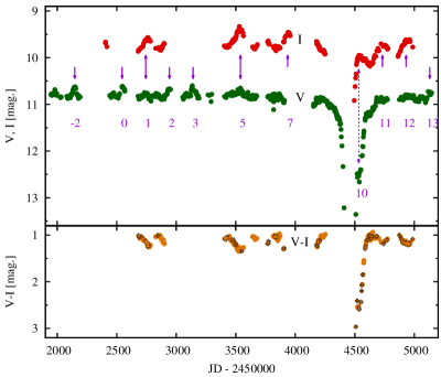
Figure 1: Top: $V$- and $I$-band light curves from ASAS-3. Bottom: the $V-I$ colour index. Crosses denote colour indices $V-I$ obtained by interpolation in the cases when $V$ and $I$ measurements were not simultaneous, i.e. not taken during the same nights. Arrows and numbers show the moments of the pulsation maxima visible in $V$- and $I$-band light curves, used for timing analysis of pulsations (see Sect. 3.2). The dotted arrow shows a postdiction for the pulsation maximum at epoch $E_{\mathrm{p}}=10$ (corresponding to a maximum that occurred during the most recent eclipse — epoch $E=8$) according to the ephemeris from Eq. 4.

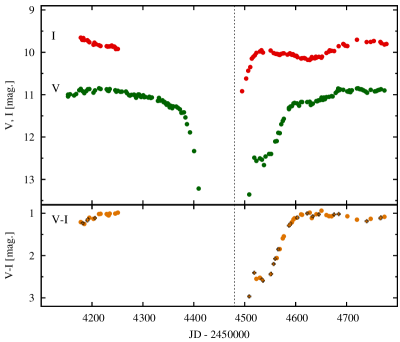
Figure 2: Expanded view of the 2007/8 eclipse of V383 Sco. The symbols are the same as in Fig. 1. The vertical dashed line marks the mid-eclipse moment² (Table 2).

The ASAS-3 survey (see Pojmański,, 2004) has monitored V383 Sco from the Las Campanas Observatory (Chile) with two standard filters since 6 Feb. 2001 (JD 2541947) in $V$ and since 5 Sept. 2002 (JD 2452404) in $I$. The data were extracted from the database in April 2010 and processed using the pipeline described by Pojmański, (1997). We selected data obtained with diaphragm numbers 2 and 0 in the cases of bands $V$ and $I$, respectively, which had the smallest statistical errors. The resulting $V$ and $I$-band light curves are presented in Fig. 1 with the colour index $V-I$ which has been calculated for measurements made on the same nights (marked with circles) and by interpolation of close but non-simultaneous measurements (marked with crosses). These are available as Tables LABEL:ASAS_V.dat–15 in our online Appendix.

High-resolution spectra (R=84000) of V383 Sco and the nearby long-period ($P=6545^{\mathrm{d}}$) eclipsing binary V381 Sco in the spectral range 3800–6900 ÅÅ were obtained at La Silla with the High Accuracy Radial velocity Planet Searcher (HARPS) spectrograph using the EGGS mode on two consecutive nights in mid-October 2009. The spectra were extracted and the wavelength calibrated using the HARPS pipeline. Additionally, a low-resolution spectrum was acquired at the end of October 2009 with the Grating Spectrograph with a SITe (Scientific Imaging Technologies, INC.) CCD mounted at the 1.9 m Radcliffe telescope at the South African Astronomical Observatory (SAAO). Grating number 7 with 300 lines mm^-1 and a slit width of $1\aas@@fstack{\prime\prime}5$ was used. To calibrate the spectrum, the spectrophotometric standard stars LTT 2415, LTT 7987, and LTT 9239 were used. All the data reduction and calibrations were carried out with standard IRAF procedures. The extracted and flux-calibrated spectrum of V383 Sco covers the range $\sim$3800–7700 Å with a resolving power of $R\simeq 1000$. The journal of our spectroscopic observations is given in Table 1.

Table 1: Journal of spectroscopic observations.

Star	Date	HJD (mid)	Exposure	Observat.
V383 Sco	14.10.2009	2455119.4965	900s	ESO
V381 Sco	15.10.2009	2455119.5115	1100s	ESO
V383 Sco	16.10.2009	2455120.5610	1100s	ESO
V383 Sco	31.10.2009	2455136.2602	1800s	SAAO

3 Results and discussion

3.1 The eclipses and orbital period

The $V$- and $I$-band light curves and $V-I$ colour index of the last eclipse of V383 Sco (in 2007/8) are shown in Figs. 1 and 2. There is a strong dependence of the eclipse depth on the photometric band. The mid-eclipse on 14 Jan 2008 (JD 2454480) occurred about $170^{\rm d}$ earlier than predicted from the ephemeris

$$JD_{\rm midecl}=2415450+4900\times E$$ (1)

which was constructed with the period and the moment of minimum from Swope, (1936). We have used the archival photometry of three minima observed before 1930 by Swope, (1936) (where the upper estimates and uncertain points were excluded from the analysis) and the ASAS-3 data obtained in the $V$ band for timing analyses. Table 2 lists approximate times of mid-eclipses, estimated using a slightly simplified variant of the Kwee & van Woerden, (1956) method. The residuals ($O-C$, observations minus calculations) for the times of minima were calculated using the linear ephemeris in Eq. 1, are listed in Table 2, and are marked in Fig. 3. The best linear fit to the residuals at epochs 0, 2, and 8, gives the new ephemeris

$$JD_{\rm midecl}=2415482(\pm 41)+4875.9(\pm 8.5)\times E.$$ (2)

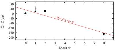
Figure 3: $O-C$ diagram with a linear (solid line) fit to the residuals. The moment of minimum at epoch 1 (vertical bar) is an estimated figure because adequate data were not available.

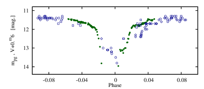
Figure 4: Light curves of four eclipses phased with a constant period according to the new linear ephemeris (Eq. 2). The open symbols denote archival photographic photometric data (squares: $E=0$, circles: $E=1$, diamonds: $E=2$). The $V$-band ASAS data (filled circles: $E=8$) have been shifted arbitrarily by $+0.6$ for facilitate comparison with the light curves from the different photometric systems.

Table 2: Moments of minima and the $O-C$ residuals estimated according to the linear ephemeris $JD_{\rm midecl}=2415450+4900\times E$.

Epoch	$JD_{\rm midecl}$=($T_{\rm Em}$)	$O-C$ [day]
0	2415453	3
1⋆	2420369–2420407	19–57
2	2425273	23
8	2454480	-170

• not used for the ephemeris fitting

It is not possible, however, to phase the light curve correctly (Fig. 4) with this new ephemeris. Regardless of which linear ephemeris is used, the eclipses are always shifted with respect to each other by up to several weeks. This makes the V383 Sco case reminiscent of the VVCep system, where the 1997 eclipse occurred by about 1% of an orbital period later than predicted (Graczyk et al.,, 1999). The reason for such large differences in eclipse contact moments is not clear, but could be due to changes in the orbital parameters. However, in the case of V383 Sco it might be appropriate to consider another possibility. The changes in the eclipse contact moments could be caused by variations in the radius of the eclipsing component caused by pulsations which could explain the observed changes in the durations of the eclipses – the eclipse at epoch $E=2$ clearly lasted significantly longer than the most recent one.

In the observational data collected so far, no traces of an eclipse of the secondary, cool component, have been detected. There is no way to predict the phase of the secondary eclipse, because through the entire orbital period the spectroscopic observations needed to infer the radial velocity curves are almost completely lacking.

3.2 Pulsations

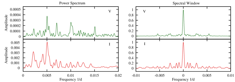
Figure 5: Power spectra obtained using Fourier analysis on out-of-eclipse $V$-band (top) and $I$-band (bottom) data (see Sect. 3.2).

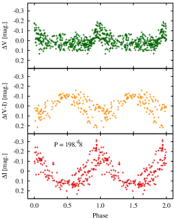
Figure 6: ASAS-3 $V$-band (top), $V-I$ (middle), and $I$-band (bottom) light curves outside of the eclipse, phased with period $P_{\mathrm{pul}}=198$ $\aas@@fstack{d}$$8$. The small amplitude of the observed $V$ variation and its strongly non-sinusoidal shape with a wide minimum are related to the presence in the system of the second component which strongly dominates in this wavelength range (see section 3.7).

The ASAS-3 photometric data outside of eclipses show apparent variations which seem to be connected with stellar pulsations. To investigate the amplitude and periodicity of these variations, we studied the out-of-eclipse data in the time intervals JD 2451947–JD 2454216 and JD 2454683–JD 2455145. After eliminating trends from the ASAS $V$, $I$ and $V-I$ data (by fitting and subtraction of a linear function and/or a second order polynomial), a fast Fourier transform was used to search for possible periods of variation.

Table 3: Frequencies and periods obtained with Fourier analysis of the out-of-eclipse $V$-band light curve. The errors $\sigma$ were estimated using the HWHM^⋆ of peaks in the power spectrum.

Frequency [1/d]	Amplitude	Period [d]	$\sigma$ [d]
0.00503	0.000375	198.8	4.8
0.01004	0.000262	99.6	1.5
0.01507	0.000182	66.36	0.49

• Half width at half maximum.

The power spectra obtained using the $V$-band data are presented in Figure 5 (top) and the frequencies and the corresponding periods are given in Table 3. The dominant frequency is the lowest strong peak at $\sim 0.00505$/d, i.e. a pulsation period of $\sim 198$ $\aas@@fstack{d}$0. A similar peak dominates in the $I$ (Fig. 5 (bottom)) and $V-I$ data, but less accurate by a factor of about two, while the peaks at greater frequencies (corresponding to shorter periods) are not visible. We therefore suggest that the period $P_{\mathrm{pul}}=198$ $\aas@@fstack{d}$$8\pm 4.8$ is a reliable value of a pulsation period for one of the components in this system. The $V$ and $I$-band light curves and variations of the $V-I$ colour index after phasing with this pulsation period are shown in Figure 6. The amplitude of variations observed in the redder $I$ band is much greater than in the bluer $V$ band.

Pulsational maxima $E_{\mathrm{p}}$ from the $V$- and $I$-band light curves, as shown in Fig. 1, were used for a second timing analysis. The moments of maxima are shown in Table 4 with their corresponding $O-C$ residuals, which were calculated using the following ephemeris

$$JD_{\rm maxPul}=2452547.5+198.8\times E_{\mathrm{p}}.$$ (3)

The pulsation zero epoch ($E_{\mathrm{p}}=0$) was adopted arbitrarily at JD 2452547.5. The best linear fit (Fig. 7) gives the ephemeris for pulsation maxima

$$JD_{\rm maxPul}=2452544.8(\pm 2.9)+198.8(\pm 0.4)\times E_{\mathrm{p}}.$$ (4)

Table 4: Pulsational maxima and the $O-C$ residuals estimated according to the initial ephemeris in Eq. 3.

$E_{\mathrm{p}}$	JD-2400000	uncertainty [d]	O-C [d]
-2	52147.0	4.5	-2.9
0	52547.5	2.0	0.0
1	52748.3	11.4	2.0
2	52943.5	4.0	-1.6
3	53134.8	4.0	-9.1
5	53529.7	6.0	-11.8
7	53941.2	3.5	2.1
8⋆	54177.8	30.0	39.9
11	54730.0	9.5	-4.3
12	54939.9	15.0	6.8
13	55123.0	6.5	-8.9

• Not used for timing analysis because of high uncertainty.

Figure 7: $O-C$ diagram for the pulsation maxima with a linear (solid line) fit to residuals.

The resulting pulsation period agrees very closely with the period calculated using Fourier analysis. The final ephemeris for pulsation maxima (Eq. 4) can be used to postdict the moment of the local maximum that indeed occurred during the last eclipse, with an accuracy of a few days, corresponding to the pulsation epoch $E_{\mathrm{p}}=10$ (see the dotted arrow in Fig. 1). It is worth noting that the photographic observations of the eclipse at epoch $E\,=\,1$ show an analogous, local pulsational maximum (see Fig. 4).

3.3 Spectral Energy Distribution (SED)

Table 5: The photometry used to calculate the spectral energy distribution (SED). The observational magnitudes and fluxes were dereddened using a colour excess $E_{\rm{B-V}}=0.46$.

Band	Wavelength	Observational		Extinction corrected		Source
	$\bar{\lambda}[$Å$]$	$[mag]$	$\sigma$	$[mag]$	$Flux[erg$ $cm^{-2}s^{-1}]$
$B_{T}$	4220	11.808	0.096	9.85	3.297e-09	TYCHO
$m_{\rm pg}$	4300	11.4	0.2	9.48	4.555e-09	Swope 1936
$V_{T}$	5353	10.656	0.062	9.20	4.279e-09	TYCHO
$V$	5450	10.790	0.012	9.37	3.535e-09	ASAS-3
$I$	9000	9.667	0.034	9.04	1.727e-09	$-_{{}^{\prime\prime}}-$
$J$	12500	8.631	0.020	8.29	1.752e-09	2MASS
$H$	16500	8.072	0.027	7.87	1.279e-09	$-_{{}^{\prime\prime}}-$
$K$	22000	7.613	0.016	7.49	8.644e-10	$-_{{}^{\prime\prime}}-$
	$\bar{\lambda}[$Å$]$	$Flux[Jy]$	$\sigma$	$Flux[Jy]$	$Flux[erg$ $cm^{-2}s^{-1}]$
9$\mu$m	90000	3.906e-01	0.082e-01	3.942e-01	1.313e-10	AKARI PSC
12$\mu$m	120000	3.632e-01	…	3.656e-01	9.134e-11	IRAS FSC
12$\mu$m	120000	4.605e-01	…	4.636e-01	1.158e-10	IRAS PSC⋆
18$\mu$m	180000	2.511e-01	0.222e-01	2.520e-01	4.197e-11	AKARI PSC
25$\mu$m	250000	2.796e-01	…	2.804e-01	3.363e-11	IRAS FSC
25$\mu$m	250000	1.118e+00	…	1.121e+00	1.344e-10	IRAS PSC⋆
60$\mu$m	600000	7.887e-01	…	7.893e-01	3.944e-11	IRAS FSC⋆
60$\mu$m	600000	5.477e-01	…	5.481e-01	2.739e-11	IRAS PSC⋆
100$\mu$m	1000000	5.090e+00	…	5.090e+00	1.526e-10	IRAS FSC⋆
100$\mu$m	1000000	1.182e+01	…	1.182e+01	3.544e-10	IRAS PSC⋆

• The IRAS PSC and FSC data have very low flux density quality, and are best considered as upper estimates.

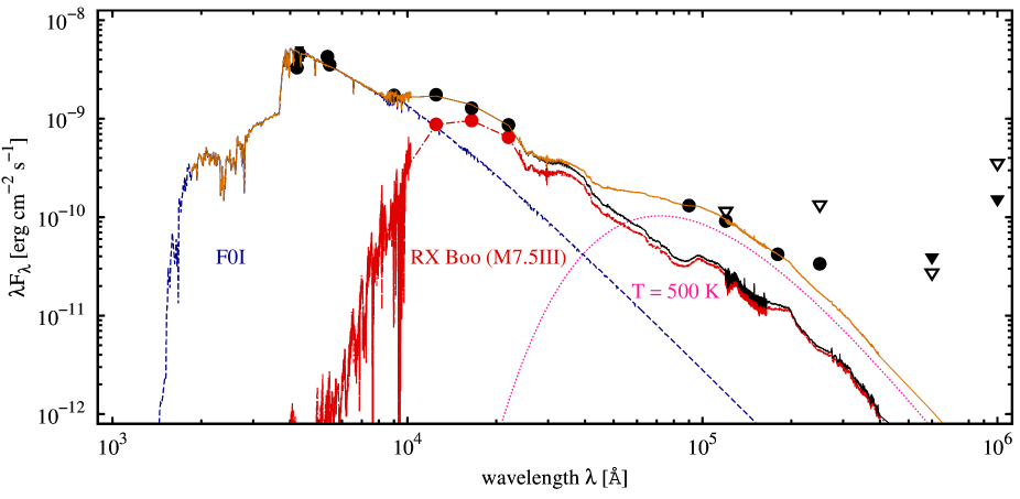
Figure 8: Dereddened spectral energy distribution of V383 Sco obtained from the data given in Table 5 (points). The dashed line (blue in the electronic version of this paper) shows the F0I-type supergiant from the 1993 Kurucz Stellar Atmospheres Atlas (Kurucz,, 1993). The dot-dashed line (red in the electronic version) marks the SED of the SRb-type pulsating star RX Boo, built using the VOSpec virtual observatory tool. The dotted line (magenta in the electronic version) shows a black body with $T$=500 K. The continuous line (orange in the electronic version) shows the sum of all 3 components appropriately rescaled (by a factor of $1.9\times 10^{-20}$ for the Kurucz model of an F0I star and by a factor of $1.3\times 10^{-4}$ for the observational SED of RX Boo) to fit the SED of V383 Sco. Triangles denote IRAS data with very low flux density quality (marked with the number 1 in the revised version of the IRAS Point Source Catalog), i.e. upper estimates: from the IRAS FSC catalogue (filled triangles) and from the IRAS PSC catalogue (open triangles).

There are not many existing photometric multicolour measurements of V383 Sco that can be used to construct its SED; however, these rare data exist over quite a wide spectral range. The TYCHO-2 catalogue has $B_{\rm T}$ and $V_{\rm T}$ magnitudes, although these are not very good quality. Inaccurate out-of-eclipse $m_{\rm pg}$ data is available from Swope, (1936). The ASAS-3 survey gives values of $V$ and $I$ magnitudes in the Johnson photometric system and 2-MASS $JHK$ observations complement the energy distribution in the near-infrared. The revised versions of the Infrared Astronomical Satellite Faint Source Catalogue (IRAS FSC) and the Point Source Catalogue (IRAS PSC) include a potential counterpart for V383 Sco. These data together with new AKARI satellite detections significantly extend the observations to the mid- and far-infrared. All the available photometric out-of-eclipse flux estimations are given in Table 5. The photometry was dereddened using the colour excess value $E_{\rm{B-V}}=0.46$ (see section 3.6) and by adopting the mean interstellar extinction curve for $R=3.1$ developed by Fitzpatrick, (2004). The magnitudes from $B_{\rm T}m_{\rm pg}V_{\rm T}VIJHK$ bands were transformed to the $\lambda F_{\lambda}$ fluxes using the Bessell et al., (1998) calibration. The resulting fluxes are shown in Table 5 and the SED is shown in Figure 8. The spectrum is dominated by an F-type supergiant in the visual and there is a significant excess from the near- to far-infrared.

Table 6: Luminosities of components of the SED of V383 Sco.

component of spectrum	Luminosity $[ergs^{-1}]$	$LL_{\sun}^{-1}$
$L_{\mathrm{hot}}$	3.67 1037	9566
$L_{\mathrm{cool}}$	9.01 1036	2346
black body (500 K)	1.28 1036	334
remnant at far IR	$\sim$(0.8 – 1.9) 1036	$\sim$(200 – 500)

3.4 Low-resolution spectrum

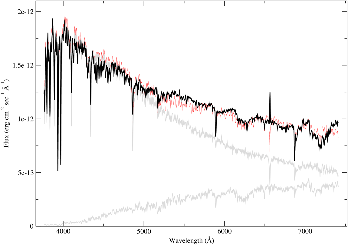
Figure 9: Observed low-resolution spectrum of V383 Sco (thick line) compared with the model (thin line) that is a superposition of F0 and M1 supergiant spectra (grey lines). The observed spectrum and the model are dereddened by $E_{\mathrm{B-V}}=0.5$.

A first inspection of the low-resolution spectrum (LRS) of V383 Sco revealed that it is dominated by a late A- or early F-type absorption spectrum. Only H$\alpha$ appears as a weak emission. In the red part of the spectrum, above $\lambda\sim 5500$ Å, traces of molecular bands seem to be present. It was obvious that the V383 Sco spectrum is a superposition of a relatively hot A–F spectrum and a cool M spectrum. In an attempt to better define both components’ spectra, we used the FITSPEC task, from the STSDAS.SYNPHOT package in IRAF, with three free variables — the renormalization of the two spectra and $E_{\mathrm{B-V}}$. The task searches for values of those variables that minimize the residuals between the templates and the observed spectrum. As templates we used the spectra from the Jacoby-Hunter-Christian spectrophotometric atlas (Jacoby et al.,, 1984) which have a resolution similar to that of our spectrum. The best model was obtained for a superposition of F0 I and M1 I spectra with a flux ratio $F_{\mathrm{F}}/F_{\mathrm{M}}=3.9$ reddened by $E_{\mathrm{B-V}}=0.5$. The observed spectrum of V383 Sco and the fitted model are compared in Fig. 9. The differences between the models for spectra in the ranges A9 I – F3 I and M1 I – M2 I (not every spectral subclass has a template in the atlas) are very small and the estimate of $E_{\mathrm{B-V}}$ varies from 0.4 to 0.6. Based on the LRS, we can infer that the spectra of the components visible in the V383 Sco spectrum are F0 I and M1 I with an accuracy of the order of one or two subclasses and that the reddening in the direction of the star is $E_{\mathrm{B-V}}=0.5\pm 0.1$.

3.5 High-resolution spectra

A careful examination of the HARPS spectra of V383 Sco obtained on 2009 October 14 and 16 did not show any noticeable night-to-night changes. Thus, we average the high-resolution spectra, obtaining a high-resolution spectrum (hereafter, HRS) with a higher S/N ratio. Comparing the V383 Sco spectrum with those from the UVES library of high-resolution spectra (Bagnulo et al.,, 2003) we found that it falls somewhere between the A9 I and F2 I spectral classes (Fig. 10). The spectrum of V383 Sco is very close to one of the spectra of $\varepsilon$ Aur from the ELODIE database (Moultaka et al.,, 2004), obtained outside the eclipse on 2003 November 1 (Fig. 10). Recently, Hoard et al., (2010) classified the spectrum of the F star in $\varepsilon$ Aur as F0 II–III? (post-AGB), and pointed out that it has the appearance of an F0 supergiant. Based on the HRS, we suggest an F0 I spectral class for V383 Sco as well.

The Balmer series lines appear similar to those in the spectrum of a Be star. H$\alpha$ is present as two emission components divided by an absorption (Fig. 11). The emission components are separated by about 70 km s^-1 and the blue component is slightly stronger than the red one. The absorption seems to be a blend of two components separated by about 10 km s^-1. In H$\beta$, in addition to the same emission and absorption components, the wings of a wide absorption profile are clearly visible (Fig. 11). The radial velocities measured on the H$\alpha$ and H$\beta$ emission wings are 89 km s^-1 and 92 km s^-1, respectively. They are practically identical with the velocity of the metallic absorptions (see Section 3.6). In the profiles of the higher series members, the wide absorption dominates. Traces of emission components in the core of the wide absorption are visible only in H$\gamma$ and H$\delta$.

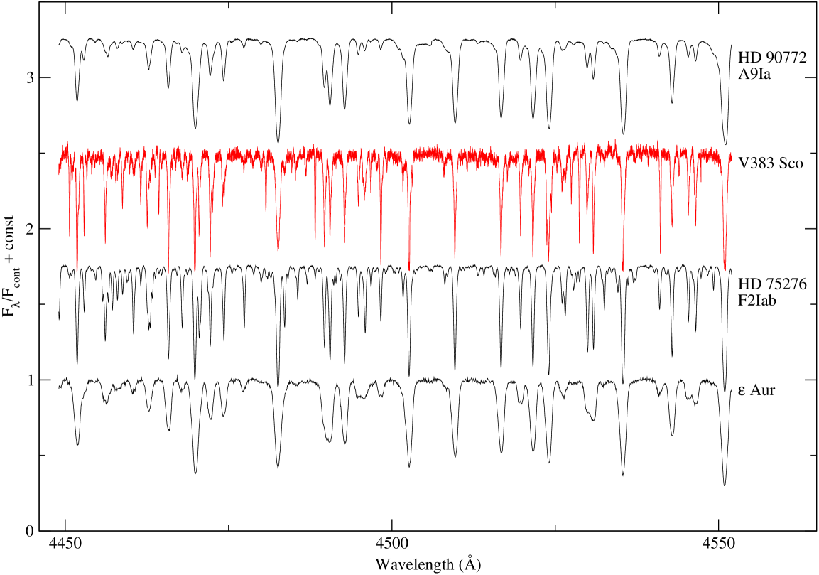
Figure 10: HARPS spectrum of V383 Sco in the region 4450–4550 Å compared with the spectra of HD 90772 and HD 75276 from the UVES library (Bagnulo et al.,, 2003) and $\varepsilon$ Aur from the ELODIE archive (Moultaka et al.,, 2004).

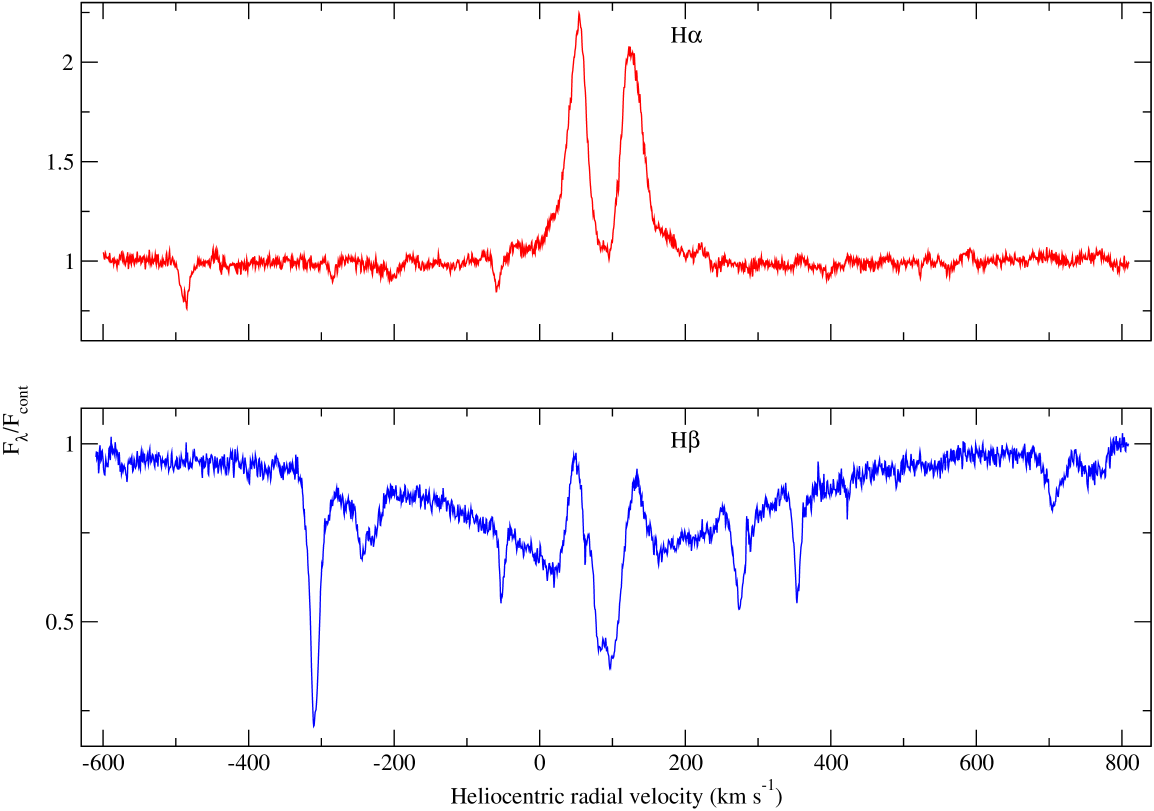
Figure 11: H$\alpha$ and H$\beta$ profiles in the HARPS spectrum of V383 Sco.

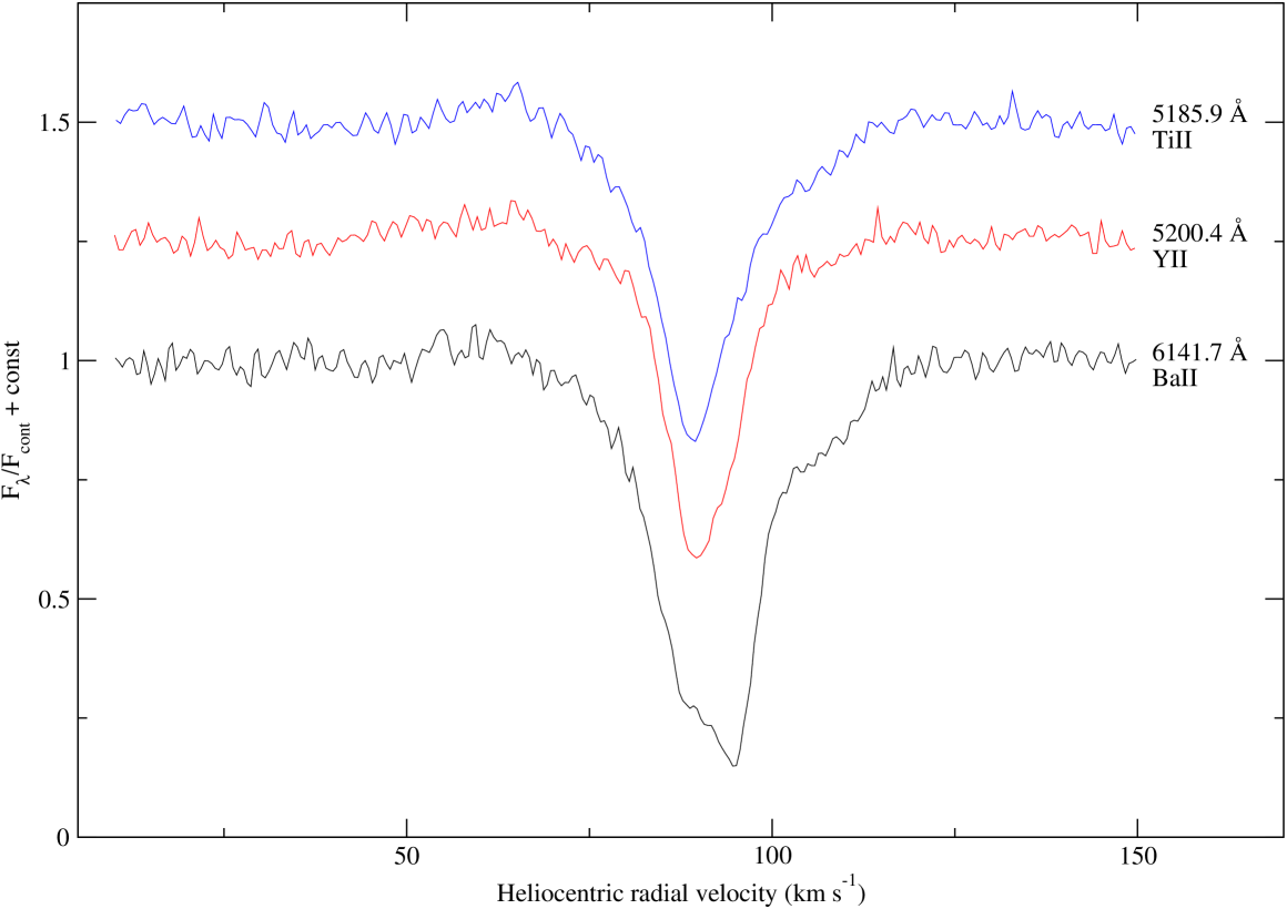
Figure 12: Profiles of Ti ii 5286 Å, Y ii 5200 Å, and Ba ii 6142 Å in the spectrum of V383 Sco in which weak emissions on the shortward edges and wide absorption wings are clearly visible.

The most common features in the spectrum of V383 Sco are sharp absorption lines of neutral and singly-ionised metals. Among the most conspicuous are the Ba ii absorptions. All the lines of multiplets 1 and 2 in our spectral region (4554 Å, 4934 Å, 5854 Å, 6142 Å, 6497 Å) are present and are among the strongest features. The Sr ii lines 4078 Å and 4216 Å are strong as well. In contrast, we were not able to identify the Li i line 6708 Å in our spectrum with S/N$\sim$35 in this region. The strongest metallic absorptions show asymmetric or split cores which indicate that they could be blends of two components (see for example the Ba ii 6142 Å line in Fig. 12 and the stellar Na i absorptions in Fig. 13). Some lines show weak, inverse P Cyg profiles with a faint blue emission component and wide absorption wings (Fig. 12). Such variety of structures shows that the spectrum of V383 Sco is very peculiar and more observational material is necessary for its better understanding.

To estimate the projected rotational velocity of the F star we used the method described by Carlberg et al., (2011). We divided the spectrum of V383 Sco in the region 4500–5500 Å into eight intervals, avoiding H$\beta$ and the interchip gap around 5320 Å. In each interval, the spectrum of V383 Sco was cross-correlated with a synthetic spectrum ($T_{\mathrm{eff}}=7500$ K, $\log g=1.5$, microturbulent velocity 1 km s^-1) from the POLLUX database (Palacios et al.,, 2010). To correct for the instrumental width, telluric lines were used. Because the macroturbulent velocity for luminosity class I, estimated from Fig. 17.10 in Gray, (2005), appeared to be higher than the total broadening, we used the formula for luminosity class II developed by Hekker & Meléndez, (2007). We found a projected rotational velocity $v\,\mathrm{sin}i=7.6\pm 0.5$ km s^-1 for the F star in V383 Sco. The reliability of this estimation is qualitatively supported by Fig. 10. It is obvious in the figure that the lines in the spectrum of V383 Sco are sharper than those in the spectrum of HD 75276. De Medeiros et al., (2002) estimate $v\,\mathrm{sin}i=9.8$ km s^-1 for HD 75276.

In addition to the emissions in the strongest Balmer lines and the very weak emission components in the inverse P Cyg profiles in the HARPS spectrum of V383 Sco, we also identified the [O i] 6300 Å and 6364 Å forbidden emissions (Fig. 14). The 6300 Å line is blended with two telluric lines, but is clearly visible while the 6364 Å line is very weak. Both [O i] forbidden emissions are shifted longward with a velocity of $\sim 90$ km s^-1 which equals the radial velocity of the absorption lines in the spectrum of V383 Sco (see Section 3.6). A Gaussian fit to the [O i] 6300 Å emission gives a FWHM of the order of $31$ km s^-1.

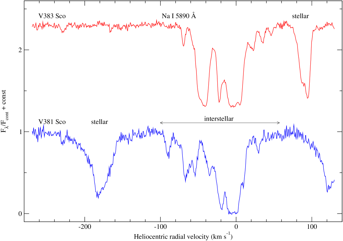
Figure 13: Comparison of the region around Na i 5890 Å in the HARPS spectra of V383 Sco (stellar absorption at around +90 km s^-1) and V381 Sco (stellar absorption at about -180 km s^-1).

3.6 Reddening and distance to V383 Sco and V381 Sco — two objects located near the Galactic centre

Like V383 Sco ($l=352\aas@@fstack{\circ}9723,\ b=06\aas@@fstack{\circ}0999$), V381 Sco ($V=12\aas@@fstack{m}3,\ l=354\aas@@fstack{\circ}2974,\ b=03\aas@@fstack{\circ}8119$) is a poorly-studied system. There are wide discrepancies in the spectral classification of this star in the literature. Its discoverer, Henrietta Swope, assigned it a spectral type F0 and an unknown luminosity class (Swope,, 1936), while Popper, (1948) classified it as an A5 Ia star. In Bowers & Kerr, (1978), V381 Sco is listed as an M5 Ia red supergiant. Comparing the spectrum of V381 Sco with the spectra from the UVES library of high-resolution spectra (Bagnulo et al.,, 2003) we found the best match with an A8 II spectrum.

In Fig. 13 we compare the region around the Na i D₂ 5890 Å line in the spectra of the two stars. It is evident that despite the proximity of the stars in the sky, the Na i interstellar line absorptions are notably different. In both spectra there are some components with similar radial velocities in the range from $-30$ to $20$ km s^-1, which most probably originate in the same interstellar clouds. Several absorptions with different radial velocities visible in the spectra indicate that additionally, there are different interstellar clouds in the direction to each star. By fitting Gaussians to the particular absorption components, we measured the total equivalent width of the interstellar Na i D₂ absorptions. Using the calibration of Munari & Zwitter, (1997), we estimated a reddening $E_{\mathrm{B-V}}=0.43$ for V383 Sco which agrees with the value obtained from the fitting of the LRS. For V381 Sco we obtained a reddening value $E_{\mathrm{B-V}}=0.39$. According to Munari & Zwitter, (1997), the accuracy of the reddening estimation based on the Na i equivalent width is higher for $E_{\mathrm{B-V}}\leq 0.4$. For multi-component profiles of Na i, as in our case, the accuracy is generally $\sim 0\aas@@fstack{m}15$. The resulting estimate of $E_{\mathrm{B-V}}$ is only a lower limit, since the Na i lines can be saturated. Hereafter, we use an average $E_{\mathrm{B-V}}=0.46\pm 0.15$ for V383 Sco.

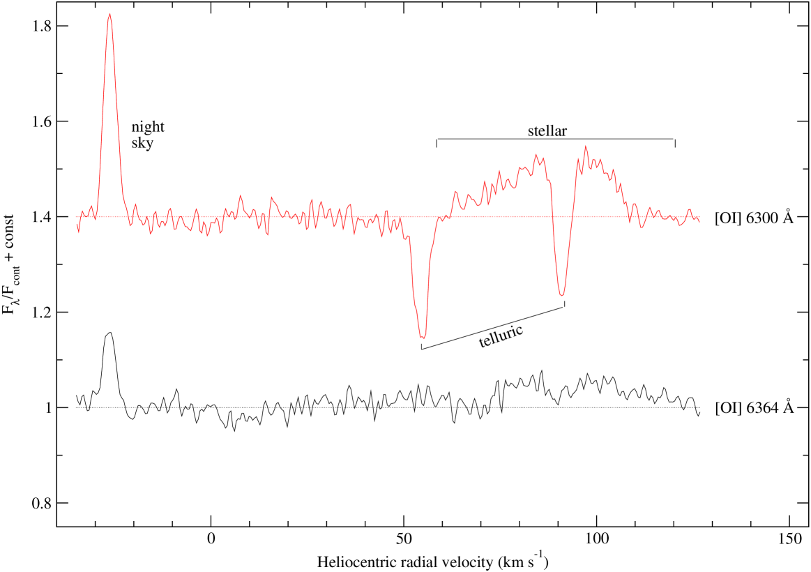
Figure 14: [O i] 6300 Å and 6364 Å forbidden emissions in the spectrum of V383 Sco.

Assuming an average out-of-eclipse brightness of V383 Sco $V=10\aas@@fstack{m}8$, a reddening $E_{\mathrm{B-V}}=0.46\pm 0.15$, and using $M_{\mathrm{V}}=5\aas@@fstack{m}1$ for an F0 Ib supergiant from Schmidt-Kaler, (1982), we derive a distance to the star of $7.8^{\mathrm{+1.9}}_{\mathrm{-1.5}}$ kpc. If we use the absolute magnitudes for F0 Ia or Iab supergiants (Schmidt-Kaler,, 1982), then the estimated distance is unrealistic and exceeds 15 kpc. Using $E_{\mathrm{B-V}}=0.39\pm 0.15$ (estimated above), an out-of-eclipse magnitude $V=12\aas@@fstack{m}3$, and $M_{\mathrm{V}}=-2\aas@@fstack{m}6$ for an A8 II bright giant (Schmidt-Kaler,, 1982), we estimate the distance to V381 Sco to be $5.5^{+1.3}_{-1.1}$ kpc.

When comparing the spectra of V383 Sco and V381 Sco we see an impressive difference in the radial velocities of the stellar absorption lines. This difference can be easily seen in the stellar Na i absorptions in Fig. 13. Using about 350 metallic absorption lines in the spectrum of V383 Sco, we measured an average heliocentric radial velocity $V_{\mathrm{h}}=89.8\pm 0.1$ km s^-1. Measuring about 190 absorption lines in the spectrum of V381 Sco, we obtained an average heliocentric velocity $V_{\mathrm{h}}=-178.8\pm 0.2$ km s^-1. The corresponding velocities relative to the local standard of rest (LSR) are $V_{\mathrm{lsr}}=98$ km s^-1 and $V_{\mathrm{lsr}}=-171$ km s^-1 for V383 Sco and V381 Sco, respectively.

The absolute velocities of both stars are high. They cannot be caused by orbital motion in such long-period systems. There is no evidence for their having a high proper motion in the literature. Most probably, these high velocities are connected with the kinematics of the regions close to the Galactic centre. V383 Sco and V381 Sco lie close to the Galactic centre and to the Galactic plane ($z\sim 0.8$ kpc and $z\sim 0.4$ kpc respectively). An examination of the Galactic-longitude–velocity diagrams of CO emission (Dame et al.,, 2001), H i (see Fig. 1 in Weiner & Sellwood,, 1999), Galactic planetary nebulae (Durand et al.,, 1998) and OH/IR and SiO-maser stars (Habing et al.,, 2006) shows that the observed velocities of V383 Sco and V381 Sco fall into regions close to the Galactic centre with very high velocities. The kinematics of the gas in these regions is inconsistent with purely circular motion (Dame et al.,, 2001; Weiner & Sellwood,, 1999, and references therein). Thus, we cannot use the standard Galactic rotation curve (e.g. Sofue et al.,, 2009) to estimate the kinematic distances of V383 Sco and V381 Sco.

Taking into consideration the distances to V383 Sco and V381 Sco estimated above, as well as their Galactic coordinates and the measured velocities relative to the LSR, both stars seem to belong to the bulge/bar structure in the inner part of the Milky Way (Weiner & Sellwood,, 1999; Habing et al.,, 2006; Vanhollebeke et al.,, 2009, and references therein). Moreover, the velocimetric model proposed by Vallée, (2008) suggests that the spatial kinematic characteristics of these stars are inconsistent with their location in any of the inner spiral arms of the Galaxy.

One way to roughly estimate the distance to V383 Sco and V381 Sco is to use the kinematic model developed by Weiner & Sellwood, (1999) for the inner part of our Galaxy. From the velocity contour plots in Fig. 8 in their paper we infer that V383 Sco is placed about 0.5 kpc behind the Galactic centre and that V381 Sco is placed about 1 kpc in front of it. For a distance to the Galactic centre $R_{\mathrm{0}}=8.0$ kpc (Sofue et al.,, 2009) the estimated distances to V383 Sco and V381 Sco are 8.5 kpc and 7 kpc, respectively. The main sources of errors in these estimates are the determination of the stars’ positions in Fig. 8 of Weiner & Sellwood, (1999) by sight and the uncertainty in the $R_{0}$ estimate (see Table 1 in Vanhollebeke et al.,, 2009). Thus, we estimate the combined random and systematic error of the kinematic distances as $\pm 1$ kpc. Thus, these distances are statistically consistent with the luminosity-based estimates indicated above.

To obtain the distance to V383 Sco by a third, independent method, we used the period–luminosity relation for pulsating Mira-type stars according to a formula given by Whitelock & Feast, (2000): $M_{\mathrm{K}}=-3.47\log{P}+\beta$ ($\beta=0.84\pm 0.14$). Using $P_{\mathrm{pul}}=198\aas@@fstack{d}8$ and dereddened infrared brightness $K_{0}=7\aas@@fstack{m}49$ we obtained a distance modulus $(K_{0}-M_{\mathrm{K}})=14.63\pm 0.20$ and a distance of $8.4\pm 0.8$ kpc. This value agrees closely with the previous two estimates ($7.8^{\mathrm{+1.9}}_{\mathrm{-1.5}}$ kpc from the $M_{\mathrm{V}}$ calibration and $8.5\pm 1$ kpc from the kinematic model of the Galactic centre). Considering these three estimates to be independent Gaussian distributions and taking a weighted mean (conservatively using 1.9 kpc as the standard deviation for the $M_{\mathrm{V}}$ estimate), we obtain $8.4\pm 0.6$ kpc as the distance to V383 Sco. Similarly, the weighted mean distance to V381 Sco from the reddening (conservatively using $5.5\pm 1.3$ kpc) and kinematic ($7\pm 1$ kpc) distances is $6.4\pm 0.8$ kpc.

3.7 Discussion of the model of V383 Sco

Our interest in V383 Sco arose from the suspicion that it could be a system similar to EE Cep and $\varepsilon$ Aur — unique long-period eclipsing binaries with a dusty debris disk as a component causing eclipses (Mikołajewski & Graczyk,, 1999). We considered the possible similarity between V383 Sco and two competing high- and low-mass models of $\varepsilon$ Aur (see e.g. Guinan & De Warf,, 2002). The analysis of the SED by Hoard et al., (2010) and conclusions drawn from interferometric observations of the disk movement relative to the F-type star by Kloppenborg et al., (2010) seem to validate the low-mass model of $\varepsilon$ Aur with a single B5V-type primary embedded in a dusty disk and a much less massive F-type post-AGB secondary. However, there still exist strong arguments in favour of the model with a high mass F-type supergiant and perhaps a binary system at the disk centre (see Chadima et al.,, 2011). We found that only the low-mass variant can be applicable to V383 Sco which explains the long-lasting eclipses ($\sim 11\%$ of the orbital period) that are observed. Nevertheless, one significant observational constraint strongly disagrees with the low-mass $\varepsilon$ Aur model. The depth of the V383 Sco eclipses shows a strong dependence on the mean wavelength of the photometric band, which is clearly visible in the $V-I$ colour index (Fig. 2). The colour changes during the eclipses exceed 2 $\aas@@fstack{m}$0, where the eclipse in the $I$ band is more than twice as shallow as it is in the $V$ band, which suggests that the eclipsing body has to contribute significantly to the total flux in the near-infrared. This case is not similar to the systems with a dark, eclipsing dusty debris disk like $\varepsilon$ Aur and EE Cep. Instead, the eclipsing object has to be a cool supergiant. A good alternative that satisfies this condition is the resemblance to the BL Tel system. In BL Tel the eclipses caused by an M-type supergiant with orbital period $P_{\mathrm{o}rb}=$778 $\aas@@fstack{d}$0 show a similar asymmetric shape to those of V383 Sco and have a similar duration of about 10$\%$ of the orbital phase (see van Genderen, 1986 and references therein, ). Pulsations with a period of 65$\aas@@fstack{d}$1 observed in BL Tel correspond to a hot component, a UU Her-type variable (van Genderen,, 1977) — a subtype of SRd-type variables. In the case of V383 Sco, however, the amplitude of the 200-day variations is higher for longer wavelengths, which has not been observed in any type of pulsating stars and is unclear given the brightness changes caused by pulsations. Thus we conclude that the pulsating component of the V383 Sco system cannot be a hot star, but rather a cool component dominating in the IR.

Another, more likely possibility is that V383 Sco is similar to HD 172481 which, according to Reyniers & Van Winckel, (2001), consists of an F-type post-AGB star and a cool M-type companion, probably AGB. Whitelock & Marang, (2001) showed that the cool component in this system is a Mira-type variable with a pulsation period of 312^d.

Several arguments can be considered in favour of the post-AGB nature of the F0 I component in V383 Sco: (i) the system’s location in the bulge/bar structure of our Galaxy; (ii) the high radial velocity; and (iii) the presence of dust that would explain the IR excess in the SED (Fig. 8). Additionally, the [O i] 6300 Å emission in the spectrum of V383 Sco may indicate the presence of a very low excitation nebula. If we assume that the wide and asymmetric profile of this forbidden line originates in an expanding nebula, then the observed outflow velocity will be of the order of 15 km s^-1, which is typical for post-AGB expanding envelopes. Nevertheless, the infrared excess observed in the SED is a little too low to be a post-AGB star.

However, much stronger arguments favour the hypothesis that there is a cool, pulsating M-type component in the V383 Sco system. Two arguments follow from the spectral energy distributions, on the basis of spectra and/or photometric data: (i) In Fig. 9 in the red part of the low-resolution spectrum there are traces of molecular absorption band features characteristic of an M-type supergiant. The spectrum in the visual domain can be fitted with a combination of an F0I and an M1I spectrum. (ii) There is an infrared excess visible in the SED (see Fig. 8). At first glance, one might suspect that the system includes a very cool non-stellar component as the companion of the F-type star that cause the eclipses. If we apply the black-body approximation to the SED in the near IR part, it may seem that the observed excess could not be produced by a cool star. However, as a consequence of efficient mass loss accompanied by dust creation, pulsating Miras or semiregular SR-type stars have SEDs with maxima strongly shifted to the near infrared with respect to a black body of the same temperature (see Lobel et al.,, 1999). Thus the observed SED of V383 Sco can be reproduced by a superposition of two stellar spectra — a hot supergiant of F0I-type and a cool M-type giant/supergiant. In Figure 8 we compared an SED of V383 Sco with the sum of the two spectra, individually rescaled to match the observed absolute flux levels, and a black body with a temperature of 500 K to explain the excess in the range up to 18 $\mu$m. The F0I-type spectrum is from the 1993 Kurucz Stellar Atmospheres Atlas (Kurucz,, 1993). The spectrum of the SRb-type star RX Boo (Fig. 8) was built using the VOSpec virtual observatory tool . According to the GCVS database RX Boo is an SRb-type star that varies with an amplitude of $\sim$2 $\aas@@fstack{m}$5 in the $V$-band and changes spectral type at least in the range M6.5e–M8IIIe with a typical period of $P_{\mathrm{pul}}=162$ $\aas@@fstack{d}$3. The presence of a cool star such as RX Boo is sufficient to reproduce the observed SED of the V383 Sco system.

There ara two more arguments for the presence of an M-type supergiant in the V383 Sco system, which provide additional evidence for pulsations of this component, come from the photometric behaviour. (iii) The eclipse depth strongly depends on the colour, i.e. on the mean wavelength of the photometric band, which shows that a cool and very bright object dominates in the near IR. (iv) The observed amplitude of pulsations is much smaller at shorter wavelengths. Using the out-of-eclipse light curves, we estimate amplitudes of the pulsation related variations as 0 $\aas@@fstack{m}$41 and 0 $\aas@@fstack{m}$21 for the $I$ and $V$ bands, respectively (see Table 7). Normally the amplitude of pulsations decreases towards longer wavelengths, but in this case it is the opposite. This can be explained by the amplitude of pulsations in short wavelengths being substantially “suppressed” by the presence of a much brighter (in the visible range) F-type supergiant. We are not sure how deep the eclipses really are because the minima were not covered during the eclipses. However, by extrapolating the changes near the mid-eclipse during the most recent epoch we estimate that the apparent magnitudes during the minimum should not be greater than about 11 $\aas@@fstack{m}$1 and 14 $\aas@@fstack{m}$3 for the $I$ and $V$ bands, respectively. If we estimate the mean magnitudes in the minima of pulsations as 9 $\aas@@fstack{m}$83 and 10 $\aas@@fstack{m}$86 for $I$ and $V$, and assume that eclipses are total, we can estimate that the flux ratios of both components $F_{\rm M}/F_{\rm F}$ change during the pulsation cycle in the range 0.444–1.107 in $I$ and 0.044–0.267 in $V$. The upper value 0.267 agrees closely with the upper value from the LRS in the visible domain obtained around the maximal phase of pulsations: $F_{\rm F}/F_{\rm M}=3.9\Rightarrow F_{\rm M}/F_{\rm F}=0.256$ (see Sec. 3.4). Hence, the amplitudes of pulsations of the cool M component could reach about $1$ $\aas@@fstack{m}$0 and $2$ $\aas@@fstack{m}$0 in the $I$ and $V$ bands, respectively, stronger in the shorter wavelengths as is expected for a pulsating star. In this case the cool component could be a semiregular, SR-type pulsating star. The estimated amplitude of pulsations strongly depends on the depths of eclipses. With increasing eclipse depth, the ratio $F_{\rm M}/F_{\rm F}$ will decrease and this is reflected by a higher amplitude of pulsations of the M-type component. Indeed, the observed SED suggests that the ratio of the components fluxes $F_{\rm M}/F_{\rm F}$ in the $I$ band could be a few times (roughly an order of magnitude) lower than estimated from the photometric data. The true amplitude of pulsations could in fact be much higher and the pulsating component could well turn out to be a Mira-type star. Very high amplitude pulsations could provide an explanation for the changes of eclipse contact moments observed during different cycles, which can result from the variations of the pulsating supergiant radius. It could also explain the observed local maxima, visible during eclipses (e.g. at $E=1$ and $E=8$) as a consequence of an increase in the cold component’s flux (caused by pulsations) together with a decrease of the hot component’s flux (caused by obscuration).

Table 7: Estimated minimum values of the eclipse depths ($M_{\rm midecl}^{\star}-\bar{M}_{\rm out}$) and the pulsation amplitudes $\delta$.

Band	$\delta$	$\delta_{\rm min}$	$\delta_{\rm max}$	$\bar{M}_{\rm out}$	$M_{\rm midecl}^{\star}$
$I$	0.41	+0.15	-0.26	9.68	11.1
$V$	0.21	+0.07	-0.14	10.79	14.3

• from extrapolation

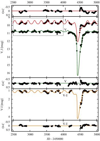
Figure 15: Synthetic $V$- and $I$-band light curve and $V-I$ colour index curves obtained by modelling, plotted with solid lines (green, red, and orange, respectively in the electronic version of this paper), in comparison with observational photometric data. Between the flux and colour curves, residuals are shown. The model assumes a temperature of the cool star $T_{\mathrm{cool}}$=2800 K. The expanded view of the out-of-eclipse $V$ and $I$ light curves (box with a dashed line) is shown in Fig. 16.

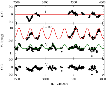
Figure 16: Expanded view of the synthetic fit to the out-of-eclipse $V$ and $I$ light curves and residuals.

We have prepared a model of the 2007/8 eclipse of V383 Sco taking into account the pulsations of the cool component using our own simple computer code. Our model is extremely simplified — the stars are considered as ideal spheres, limb darkening has been neglected, and stellar fluxes are approximated as black bodies. The changes in the radius of the M-type supergiant and in its brightness have been expressed with cosine functions. A more detailed description of the model assumptions and the parameters that have been derived are presented in the online Appendix A. As inputs to the model we assumed that the hot component has an effective temperature $T_{\mathrm{cool}}=7500$ K and its radius $R_{\mathrm{hot}}=58\,R_{\sun}$ was estimated using the Stefan-Boltzman law by adopting the luminosity $L_{\mathrm{hot}}$ extracted from the SED (see Table 6). The best solution was found for the M supergiant at effective temperature $T_{\mathrm{cool}}=2800$ K and with radius $\bar{R}_{\mathrm{cool}}=208\,R_{\sun}$, which is changing due to the pulsations by $\Delta R$ = $\pm$0.19$\bar{R}_{\mathrm{cool}}$. In our model the supergiant totally obscures the hot component during an eclipse minimum. The resulting amplitudes of the brightness changes in the cold supergiant — if it were observed as a solitary star — would be 3$\aas@@fstack{m}$66 and 1$\aas@@fstack{m}$75 in the $V$ and $I$ bands, respectively. The synthetic $V$- and $I$-band light curves and $V-I$ colour index curve are shown in Figure 15 and compared with photometric observational data. The eclipse is very deep, about 5$\aas@@fstack{m}$6 in $V$ and 2.5 in $I$ and needs to be confirmed by future observations, because the system has never been observed at the exact moment of minimum. It will be necessary to organize an observational campaign for the next eclipse in order to obtain data with a dense sufficiently time coverage. With the parameters of the system components derived from our model, we estimate that if a secondary eclipse occurs, it would be very shallow, i.e. a few 0$\aas@@fstack{m}$001 in the $V$ band and not deeper than about 0$\aas@@fstack{m}$02 in $I$. Given the strong changes in brightness caused by pulsations that are quite irregular in terms of amplitude it is rather certain that the secondary eclipse will be undetectable in the visible range. The situation is somewhat better in the near-infrared ($JHK$ bands), where we estimate that the eclipse depths should fall in the range 0$\aas@@fstack{m}$04–0$\aas@@fstack{m}$06, though this would still be very difficult to observe. Careful inspection of Figure 16 reveals an additional interesting feature in the synthetic light curves. To our surprise and satisfaction, our model has reproduced flattened pulsational minima in the synthetic $V$-band light curve, which we had noticed in the phased observational $V$-band light curve (see Fig. 6, top) without understanding the origin of this phenomenon. Now we know that this is the natural consequence of the fact that the pulsating star is a component of a system with an object which strongly dominates in a given photometric band. The changes which look roughly sinusoidal for a single pulsating star will have flattened minima when we put the pulsating star in a binary system together with a much brighter star. This result can constitute the additional, fifth (v) argument to support the proposed model of V383 Sco with a pulsating cool supergiant as the eclipsing component. The best results are obtained with a low temperature of the cool component, $T_{\mathrm{cool}}=2800$ K, which agrees very closely with the result for the M star based on the SED. The unreddened $V-I$ colour index close to the mid-eclipse is approximately 4$\aas@@fstack{m}$0, which is close to the index expected for a M7-8 star. We found earlier (Sect. 3.4, Fig. 9) that the M star was better described by an M1-type fit to the low-resolution spectrum. The difference between M1 and M7-8 is significant and corresponds to a temperature difference of about 700–800 K. On the other hand, the low-resolution spectrum was obtained at a pulsational maximum (on 31 Oct. 2009 – JD 2455136), according to the ephemeris from (Eq. 4) at a pulsation phase almost exactly equal to zero ($\sim$0.03). At that time, the star had reached the temperature close to the maximum possible value of the pulsation cycle. Thus, the results are consistent with our model, because during its pulsations, the cool star changes its spectral type, at least in the range from about M1 to about M7–8.

4 Conclusions

Using the ASAS-3 photometric data together with high (HARPS) and low (1.9 m telescope at SAAO) resolution spectra, we have revised our knowledge of the long-period eclipsing binary V383 Sco, for the first time since the 1930s. Contrary to our initial expectations, the system does not resemble the unique systems with dusty debris disks as eclipsing bodies, neither the famous, very long period eclipsing binary $\varepsilon$ Aur, nor EE Cep. Instead, we have found a number of arguments in favour of a new model in which V383 Sco could be similar to HD 172481 — a system with a post-AGB F0-type star and a cool, pulsating M-type supergiant. The most important difference between these systems lies in the orientation of the orbits which enables the observation of eclipses only in the case of V383 Sco. While the hot component in V383 Sco shows some features characteristic of post-AGB stars, the detected infrared excess is too small and we can say with certainty that it is a supergiant of spectral type approximately F0. However, in the case of the second component that causes the eclipses, we found strong evidence that it is a cool, pulsating M-type supergiant on the basis of the following arguments:
i) Traces of molecular absorption bands, characteristic of an M-type supergiant, are present in the red part of the low-resolution spectrum
ii) The observed SED can be reproduced by the superposition of two stellar spectra, a hot supergiant of F0I-type, and a cool M-type giant/supergiant
iii) the eclipse depth strongly depends on the photometric band — it decreases in the direction of increasing wavelength
iv) The pulsation amplitude is lower in the shorter wavelength band
v) The flattened “bottoms” of the pulsation minima observed in the $V$ band are consistent with a synthetic model of the eclipses.
In addition, the presence of the pulsating supergiant in the system could explain the changes in duration and shape of the eclipses.

The forbidden emission [O i] 6300 Å in the HRS indicates the presence of a very low excitation nebula around the V383 Sco system.

V383 Sco and a similar eclipsing binary V381 Sco (by chance located close to each other in the sky), have very high and oppositely directed radial velocities: $89.8$ km s^-1 vs $-178.8$ km s^-1. These are in agreement with the kinematics of the regions close to the Galactic centre. V383 Sco and V381 Sco lie close to the Galactic centre and to the Galactic plane ($z\sim 0.8$ kpc and $z\sim 0.4$ kpc, respectively). The distance to V383 Sco estimated using reddening, radial velocities, and the period-luminosity relation is 8.4 $\pm$0.6 kpc. The distance to V381 Sco estimated from the reddening and kinematic distances is $6.4\pm 0.8$ kpc.

The observational material collected so far is just sufficient to construct a rough model of the V383 Sco system, which reproduces the main features of observed photometric changes in the $V$ and $I$-band light curves. With our model we obtain very deep eclipses: about 5$\aas@@fstack{m}$6 in $V$ and 2$\aas@@fstack{m}$5 in $I$. This result requires confirmation by future observations, as the exact moment of minimum has never been observed.

The next eclipse should start in the middle of 2020. It is important to carry out an extensive photometric and spectroscopic campaign to observe it. In the meantime, systematic spectroscopic monitoring would be useful to obtain a spectroscopic orbit, with which it would became possible to obtain a more precise estimate of the basic parameters of the system’s components such as their masses and radii. Simultaneous photometric observations would be still valuable for the study of changes in the M-type supergiant radius as a function of the pulsational phase. Observational material obtained for this object over a decade time scale is still quite scant and any additional data should lead to very valuable and interesting results.

Appendix A Simple model of V383 Sco

To make the model of the 2007/8 eclipse of V383 Sco, which we describe briefly below, many simplifying assumptions were made. Stars were considered as spheres with radii $R_{\mathrm{hot}}$, $\bar{R}_{\mathrm{cool}}$ and effective temperatures of photosferes $T_{\mathrm{hot}}$, $T_{\mathrm{cool}}$ for the hot F-type and cool M-type components, respectively. Limb darkening was neglected and stellar fluxes were approximated as black bodies. We describe the main eclipse (of the hot component by the cool supergiant) by taking into account an impact parameter $D$ which measures the projected distance between the centres of stellar disks at the mid-eclipse point, as well as changes in the radius of the cool star in the range $\pm\Delta R$ from the mean value of the radius $\bar{R}_{\mathrm{cool}}$ as a result of the pulsations (Fig. 17). Pulsational changes in the radius and brightness of the cool component were described simply, similar to the approach used for modelling pulsations in Mira $\chi$ Cyg by Reid & Goldston, (2002). In our model we assume that the changes in magnitudes and radius of the cool star can be expressed with cosine functions

$$M_{\mathrm{cool}}=\bar{M}_{\mathrm{cool}}+\Delta M\cos{(\phi_{\mathrm{pul}})},$$ (5)

$$R_{\mathrm{cool}}=\bar{R}_{\mathrm{cool}}+\Delta R\cos{(\phi_{\mathrm{pul}}+\Delta\phi_{\mathrm{pul}})},$$ (6)

where $\Delta M$ is the semi-amplitude of brightness changes caused by pulsations (from the mean value), $\phi_{\mathrm{pul}}$ is a pulsation phase, and $\Delta\phi_{\mathrm{pul}}$ is a phase shift which expresses by how much the moment of maximum radius of the M star precedes the moment of maximum of its brightness. The period and zero moment of pulsation maxima were adopted from the ephemeris (Eq.4). Several parameters were treated as fixed, not subject to change in the process of solution. The effective temperature of the hot component $T_{\mathrm{hot}}$ was set to 7500 K and its radius $R_{\mathrm{hot}}=58R_{\sun}$ was estimated with the Stefan-Boltzmann law by adopting the luminosity $L_{\mathrm{hot}}$ extracted from the SED (see Table 6). The broad, atmospheric parts of the eclipse were included by introducing a light-absorbing envelope that changes the density distribution as a function of distance from its centre $r$ as $r^{-2}$. Its radius $R_{\mathrm{env}}$ was roughly estimated from the total duration of the atmospheric eclipse and fixed at 440 $R_{\sun}$. We assumed that the intensity of radiation $\mathbb{I}$, measured after passing through the envelope, changes from an initial value $\mathbb{I}_{0}$ according to

$$\mathbb{I}=\mathbb{I}_{0}\,e^{-\tau(r)},$$ (7)

where $\tau(r)$ is an optical depth calculated

$$\tau(r) = 2\int_{\mathrm{z}=0}^{\sqrt{R_{\mathrm{env}}^{2}-r^{2}}}\,\kappa\,\rho(r,z)\,dz$$ (8)

$$= 2\,C\,\kappa\,r^{-1}\arctan{\left(r^{-1}\,\sqrt{R_{\mathrm{env}}^{2}-r^{2}}\right)}.$$

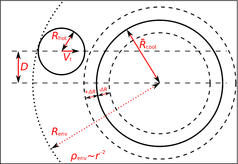
Figure 17: Schematic explanation for the geometric parameters of the model.

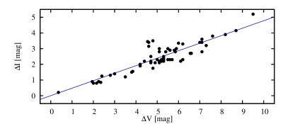
Figure 18: Dependence of the pulsation amplitude of Mira/Semi-Regular pulsating stars in the $V$ photometric band on the amplitude in the $I$ band obtained from AAVSO light curves.

The absorption coefficients $\kappa_{\mathrm{V}}$ and $\kappa_{\mathrm{I}}$ were chosen via visual comparison of synthetic curves with photometric observational data and were fixed at the values 0.03 and 0.015 for $V$ and $I$ bands, respectively, assuming that the integration constant $C$ is equal to 1. We carried out the solutions for several temperatures of the cool component $T_{\mathrm{cool}}$ in the range from 2600 K to 3500 K with a step of 100 K. For each $T_{\mathrm{cool}}$ value we calculated the star’s radius $\bar{R}_{\mathrm{cool}}$ from the Stefan-Boltzmann law using the luminosity extracted from the SED from the spectrum of RX Boo fitted in the place of the cool component (see Table 6). The adjustable, free parameters were: the moment of mid-eclipse defined as the time at which the centres of stellar disks are at the minimum separation $JD_{\mathrm{0}}$, the reciprocal tangential velocity of the stars $V_{\mathrm{t}}$, the semi-amplitude of brightness changes caused by pulsations $\Delta M_{\mathrm{V}}$, $\Delta M_{\mathrm{I}}$ for $V$ and $I$ bands, respectively, and three parameters described earlier: $D$, $\Delta R$, and $\Delta\phi_{\mathrm{pul}}$. To reduce the number of free parameters we combined the semi-amplitudes of $\Delta M_{\mathrm{V}}$, $\Delta M_{\mathrm{I}}$ using an empirical relationship $\Delta M_{\mathrm{I}}\approx 0.478\,\Delta M_{\mathrm{V}}$ that we found when analysing the AAVSO photometric data for Miras- and SR-type stars (see Fig. 18). The best solution, i.e. corresponding to the minimum value of the sum of square residuals, was obtained for $T_{\mathrm{cool}}=2800$ K and $\bar{R}_{\mathrm{cool}}=208\,R_{\sun}$. The complete set of resulting parameters of the model is shown in Table 8.

Table 8: Input (left) and output (right) parameters of the model of the 2007/8 eclipse of V383 Sco.

INPUT			OUTPUT
Parameter	Value	Unit	Parameter	Value	Unit
$T_{\mathrm{hot}}$	7500	K	$T_{\mathrm{cool}}$	2800	K
$R_{\mathrm{hot}}$	58	$R_{\sun}$	$\bar{R}_{\mathrm{cool}}$	208	$R_{\sun}$
$R_{\mathrm{env}}$	440	$R_{\sun}$	$\Delta R$	$\pm$0.19	$\bar{R}_{\mathrm{cool}}$
$\kappa_{\mathrm{V}}$	0.03	1	$D$	108	$R_{\sun}$
$\kappa_{\mathrm{I}}$	0.015	1	$\Delta M_{\mathrm{V}}$	1.83	mag
			$\Delta M_{\mathrm{I}}$	0.875	mag
			$JD_{\mathrm{0}}$	2454479	day
			$V_{\mathrm{t}}$	1.349	$R_{\sun}$ day-1
			$\Delta\phi_{\mathrm{pul}}$	0.24	1

Appendix B Online photometric data

Table 10: Photometric data obtained from the ASAS-3 survey in $V$ band. The column labelled “Grade” shows the quality flags, where A denotes the highest quality of measurements and D the lowest.

$HJD-2450000$	$V$	ErrV	Grade	$HJD-2450000$	$V$	ErrV	Grade	$HJD-2450000$	$V$	ErrV	Grade
1947.88374	10.794	0.038	A	3059.85594	10.891	0.034	A	4266.72275	10.926	0.048	A
1950.86934	10.776	0.042	B	3062.88171	10.873	0.098	D	4268.72660	10.965	0.047	A
1954.87335	10.778	0.039	A	3067.89681	10.850	0.033	A	4272.65519	11.012	0.030	A
1955.85720	10.808	0.033	A	3075.86116	10.779	0.034	A	4274.68990	11.022	0.031	A
1961.88650	10.781	0.037	A	3080.85228	10.820	0.036	A	4277.66524	11.004	0.029	A
1963.86687	10.789	0.033	A	3086.89861	10.763	0.033	A	4282.68026	10.999	0.038	A
1965.86244	10.790	0.032	A	3090.83658	10.798	0.039	A	4284.68381	11.024	0.032	A
1967.86500	10.794	0.036	A	3096.91284	10.789	0.033	A	4286.67763	11.072	0.040	A
1978.81197	10.743	0.043	A	3099.83336	10.827	0.036	C	4290.67641	10.996	0.031	A
1979.84605	10.685	0.041	A	3102.85879	10.831	0.038	A	4292.65072	10.997	0.030	A
1980.82505	10.723	0.043	A	3107.89134	10.828	0.035	A	4294.65876	11.038	0.038	A
1981.84012	10.714	0.040	A	3113.80802	10.817	0.032	A	4296.64837	11.055	0.034	A
1982.80377	10.713	0.043	A	3114.71911	10.796	0.040	A	4298.65374	11.031	0.032	A
1994.78866	10.809	0.045	B	3116.79617	10.806	0.034	A	4300.61757	11.015	0.042	A
1997.80247	10.775	0.048	B	3122.82749	10.817	0.030	C	4302.66254	11.059	0.030	A
2025.75974	10.857	0.038	A	3125.75038	10.707	0.037	A	4304.61034	11.053	0.029	A
2032.76086	10.839	0.036	A	3127.74793	10.681	0.043	A	4310.60157	11.067	0.033	A
2033.75875	10.845	0.037	A	3129.79093	10.673	0.052	B	4312.59860	11.049	0.038	A
2080.59240	10.825	0.051	D	3130.88156	10.632	0.037	A	4315.60113	11.077	0.029	A
2083.64911	10.840	0.043	A	3134.80681	10.613	0.033	A	4317.65819	11.066	0.030	A
2087.63899	10.874	0.048	B	3134.81947	10.601	0.033	A	4329.53502	11.147	0.038	A
2103.61244	10.821	0.042	A	3144.75345	10.690	0.033	A	4331.53698	11.076	0.028	A
2109.60174	10.861	0.037	A	3152.86228	10.725	0.035	A	4333.53333	11.140	0.032	A
2115.57163	10.786	0.037	A	3154.70184	10.718	0.032	A	4338.51434	11.133	0.030	A
2116.57664	10.815	0.037	A	3162.70343	10.723	0.032	A	4340.57579	11.176	0.033	A
2117.57550	10.792	0.039	A	3164.73369	10.732	0.033	A	4342.58047	11.172	0.033	A
2124.55146	10.778	0.043	A	3167.75173	10.733	0.031	A	4344.57746	11.205	0.035	A
2125.56730	10.773	0.042	A	3169.72032	10.767	0.032	A	4346.57994	11.239	0.033	A
2130.56789	10.721	0.037	A	3171.85324	10.795	0.055	B	4348.58159	11.206	0.032	A
2133.55142	10.696	0.040	A	3178.66149	10.813	0.037	A	4350.57676	11.231	0.035	A
2134.54494	10.683	0.040	A	3180.76054	10.868	0.037	A	4352.58899	11.300	0.030	A
2135.54601	10.678	0.039	A	3183.74281	10.815	0.034	A	4355.57806	11.267	0.033	A
2140.51371	10.639	0.047	B	3191.74947	10.867	0.040	A	4357.58803	11.319	0.033	A
2140.52774	10.640	0.043	A	3266.53629	10.796	0.029	A	4359.55213	11.276	0.032	A
2142.51725	10.644	0.039	A	3278.60864	10.809	0.040	A	4365.49796	11.282	0.031	A
2151.49387	10.622	0.043	A	3292.53450	10.941	0.037	A	4368.57314	11.309	0.035	A
2151.51481	10.661	0.045	A	3298.50418	10.785	0.032	A	4372.59864	11.345	0.038	A
2156.48797	10.661	0.034	A	3404.88403	10.832	0.040	A	4375.60334	11.429	0.032	A
2164.47852	10.774	0.036	A	3414.88178	10.847	0.036	A	4378.50501	11.420	0.036	A
2168.54968	10.788	0.038	A	3418.87955	10.854	0.056	D	4380.56009	11.418	0.035	A
2172.48929	10.823	0.035	A	3422.86890	10.816	0.043	A	4383.53295	11.538	0.029	A
2178.48638	10.873	0.038	A	3426.86242	10.784	0.040	A	4386.51811	11.697	0.030	A
2180.53133	10.864	0.037	A	3446.88537	10.785	0.033	A	4392.49714	11.891	0.035	A
2184.53135	10.818	0.047	B	3450.85023	10.782	0.037	A	4400.50462	12.333	0.038	A
2188.51177	10.840	0.035	A	3453.82351	10.762	0.034	A	4409.51408	13.217	0.036	A
2192.50133	10.845	0.035	A	3456.84081	10.805	0.038	A	4508.88491	13.357	0.038	A
2441.66561	10.811	0.034	A	3463.81654	10.815	0.040	A	4518.87474	12.488	0.037	A
2443.65941	10.807	0.026	A	3469.84212	10.734	0.038	A	4522.87709	12.563	0.031	A
2444.65222	10.813	0.029	A	3472.86391	10.762	0.035	A	4529.85835	12.504	0.031	A
2446.66627	10.813	0.029	A	3475.82595	10.797	0.047	A	4533.87840	12.534	0.037	A
2452.62571	10.853	0.040	A	3478.78756	10.747	0.041	A	4537.84370	12.662	0.032	A
2459.61282	10.823	0.046	A	3481.78940	10.807	0.042	A	4540.86788	12.460	0.038	A
2463.61786	10.780	0.028	A	3483.82058	10.790	0.037	A	4547.83524	12.400	0.035	A
2464.61902	10.795	0.029	A	3489.86652	10.797	0.039	A	4551.83969	12.399	0.041	A
2465.62043	10.770	0.029	A	3491.88992	10.790	0.049	B	4559.85123	12.105	0.030	A
2466.60753	10.775	0.028	A	3499.78427	10.758	0.048	A	4562.86230	12.096	0.034	A
2467.61244	10.793	0.034	A	3502.75037	10.786	0.042	A	4565.87866	11.901	0.032	A
2470.53720	10.775	0.031	A	3504.78985	10.784	0.041	A	4568.84687	11.909	0.039	A
2474.62250	10.750	0.034	A	3510.82468	10.750	0.032	A	4571.80941	11.698	0.032	A
2482.59589	10.820	0.038	A	3517.77501	10.684	0.040	A	4574.77250	11.621	0.033	A
2486.57132	10.817	0.045	B	3521.73467	10.762	0.042	A	4576.83365	11.570	0.039	A
2489.56035	10.835	0.037	A	3523.77132	10.770	0.056	D	4586.86275	11.342	0.036	A
2490.57401	10.841	0.037	A	3525.83400	10.765	0.046	B	4586.86848	11.311	0.032	A
2493.56026	10.820	0.040	A	3528.68716	10.759	0.041	A	4589.80061	11.282	0.033	A
2495.56736	10.841	0.033	A	3530.72938	10.732	0.040	A	4592.76977	11.270	0.033	A
2497.55787	10.835	0.031	A	3539.65622	10.650	0.052	D	4595.77096	11.207	0.032	A
2498.54597	10.826	0.033	A	3544.70032	10.688	0.047	D	4597.85833	11.194	0.031	A
2499.53951	10.832	0.027	A	3547.75284	10.714	0.039	A	4602.77582	11.205	0.034	A
2501.54772	10.816	0.159	D	3551.74481	10.763	0.049	B	4606.77977	11.262	0.040	A
2508.57056	10.829	0.032	A	3553.86272	10.720	0.059	D	4610.78142	11.173	0.033	A
2510.53066	10.854	0.036	A	3556.61734	10.768	0.035	A	4612.78279	11.175	0.053	B
2511.59233	10.849	0.037	A	3559.65093	10.739	0.049	D	4622.73751	11.175	0.033	A
2512.65139	10.869	0.048	A	3561.66521	10.819	0.040	A	4627.71547	11.166	0.033	A
2519.65366	10.807	0.033	A	3563.63391	10.798	0.038	A	4629.70080	11.244	0.032	A
2521.65567	10.793	0.033	A	3574.78547	10.823	0.036	A	4631.71467	11.226	0.032	A
2524.61338	10.771	0.043	B	3576.78662	10.833	0.038	A	4633.69397	11.213	0.037	A
2543.51237	10.623	0.036	A	3584.75114	10.811	0.045	D	4640.65753	11.151	0.034	A
2544.49166	10.619	0.035	A	3593.55661	10.793	0.034	A	4642.68813	11.155	0.030	A
2545.55285	10.639	0.034	A	3599.59462	10.805	0.032	A	4644.71063	11.135	0.033	A
2547.53527	10.612	0.034	A	3601.66452	10.742	0.053	B	4646.71972	11.132	0.041	A
2552.52426	10.634	0.044	B	3603.66385	10.814	0.037	A	4648.76300	11.126	0.036	A
2560.48978	10.658	0.033	A	3606.66320	10.872	0.041	A	4650.82420	11.068	0.036	A
2561.51828	10.679	0.037	A	3616.49767	10.837	0.039	A	4653.60971	11.124	0.030	A
2564.52232	10.692	0.035	A	3618.60179	10.876	0.043	A	4655.64585	11.067	0.031	A
2566.49718	10.689	0.036	A	3620.60528	10.882	0.046	D	4657.68244	11.105	0.039	A
2568.53853	10.718	0.036	A	3628.49132	10.884	0.036	A	4660.63377	11.058	0.048	A
2678.87312	10.825	0.036	A	3630.57205	10.822	0.037	A	4665.63048	11.051	0.034	A
2685.86873	10.888	0.033	A	3632.57919	10.889	0.037	A	4670.72256	11.035	0.053	B
2688.87290	10.861	0.039	A	3634.60725	10.818	0.037	A	4672.73512	11.041	0.032	A
2693.86357	10.886	0.034	A	3637.61923	10.838	0.036	A	4678.74256	10.958	0.058	D
2698.85680	10.849	0.037	A	3641.57576	10.806	0.034	A	4681.66501	10.919	0.036	A
2701.84353	10.839	0.033	A	3643.62026	10.803	0.034	A	4683.66433	10.854	0.040	A
2704.84566	10.836	0.033	A	3647.55667	10.828	0.030	A	4685.64790	10.896	0.038	A
2706.86653	10.808	0.033	A	3654.49371	10.820	0.044	A	4687.60767	10.875	0.035	C
2711.83090	10.847	0.030	A	3659.52089	10.828	0.037	A	4693.54540	10.885	0.034	A
2713.86742	10.835	0.032	A	3661.53924	10.882	0.040	A	4701.55681	10.923	0.032	A
2717.84758	10.840	0.035	A	3663.54306	10.859	0.038	A	4703.56097	10.931	0.037	A
2720.81780	10.831	0.037	A	3666.54497	10.840	0.040	A	4705.59719	10.898	0.038	A
2725.78682	10.810	0.034	A	3670.50303	10.809	0.036	A	4707.68375	10.941	0.042	A
2727.84169	10.821	0.034	A	3676.50738	10.824	0.040	A	4710.56786	10.897	0.048	A
2729.83267	10.796	0.036	A	3767.87772	10.843	0.043	A	4720.52758	10.854	0.036	A
2732.86927	10.748	0.034	A	3774.88655	10.818	0.044	A	4722.57958	10.850	0.041	A
2734.83991	10.760	0.032	A	3791.87572	10.897	0.043	A	4725.60196	10.869	0.044	A
2736.81316	10.756	0.031	A	3795.87709	10.900	0.037	A	4728.55975	10.872	0.039	A
2738.82916	10.760	0.033	A	3803.86526	10.858	0.048	A	4730.60237	10.881	0.042	B
2740.80750	10.767	0.038	A	3806.87455	10.793	0.040	A	4733.61441	10.901	0.038	A
2744.79595	10.773	0.051	B	3810.86534	10.813	0.043	A	4737.59596	10.926	0.031	A
2751.86773	10.768	0.035	A	3814.85063	10.791	0.045	A	4740.58241	10.954	0.031	A
2754.80976	10.775	0.033	A	3817.79346	11.113	0.045	A	4747.51394	10.886	0.046	B
2756.77009	10.763	0.031	A	3817.82384	10.782	0.043	A	4755.56689	10.922	0.039	A
2758.80878	10.789	0.029	A	3817.85291	10.835	0.040	A	4758.53982	10.915	0.039	A
2760.75837	10.825	0.034	A	3817.88154	10.945	0.043	A	4761.52917	10.895	0.038	A
2764.74750	10.807	0.033	A	3817.90940	10.795	0.042	A	4764.52606	10.885	0.037	A
2768.83207	10.883	0.035	A	3818.78028	10.816	0.043	A	4767.52218	10.871	0.041	A
2770.79462	10.835	0.042	A	3818.81001	10.798	0.048	D	4774.49989	10.901	0.043	B
2775.79778	10.870	0.036	A	3818.83776	10.840	0.046	A	4873.88154	10.899	0.096	D
2782.77636	10.866	0.047	B	3818.86603	10.787	0.054	B	4884.86344	10.890	0.043	A
2784.73145	10.847	0.030	A	3818.89487	10.817	0.041	A	4888.85412	10.844	0.060	D
2786.69223	10.823	0.034	A	3819.83248	10.806	0.047	A	4892.85329	10.871	0.048	A
2787.85465	10.932	0.039	A	3822.86444	10.843	0.039	A	4904.90499	10.908	0.056	D
2791.65946	10.836	0.035	A	3825.85961	10.778	0.045	A	4916.83957	10.879	0.045	A
2795.74352	10.816	0.034	A	3829.81893	10.790	0.037	A	4919.88115	10.824	0.049	B
2808.70976	10.829	0.031	A	3832.83783	10.785	0.043	A	4924.90464	10.796	0.056	D
2810.63295	10.812	0.031	A	3835.83326	10.867	0.039	A	4928.89062	10.813	0.054	B
2811.81572	10.830	0.035	A	3847.85540	10.886	0.047	A	4931.85646	10.816	0.054	B
2813.70912	10.810	0.034	A	3850.79804	10.911	0.047	D	4940.81812	10.797	0.050	B
2820.70452	10.832	0.029	A	3852.84525	10.906	0.044	A	4946.79831	10.859	0.049	A
2826.73553	10.836	0.028	A	3855.78777	10.864	0.056	D	4949.79831	10.840	0.050	B
2830.61263	10.763	0.041	A	3858.77707	10.844	0.045	A	4952.77460	10.835	0.045	A
2835.62683	10.810	0.030	A	3860.84328	10.819	0.035	A	4954.82780	10.803	0.045	A
2838.62847	10.819	0.029	A	3862.83173	10.814	0.036	A	4959.81795	10.814	0.057	D
2840.68315	10.802	0.031	A	3864.75915	10.772	0.047	D	4965.81098	10.813	0.059	D
2842.66518	10.780	0.094	D	3866.76219	10.834	0.041	A	4967.83882	10.826	0.047	A
2845.67292	10.810	0.030	A	3868.78516	10.789	0.043	A	4973.81523	10.862	0.054	D
2851.58670	10.791	0.027	A	3872.79988	10.803	0.041	A	4984.74961	10.855	0.054	B
2853.71459	10.811	0.030	A	3882.71417	10.851	0.038	A	4988.73132	10.868	0.053	B
2855.62088	10.858	0.033	A	3892.72766	10.912	0.036	A	4992.79084	10.808	0.064	D
2861.56826	10.856	0.030	A	3894.71976	10.902	0.031	A	5002.69736	10.862	0.049	A
2862.67814	10.841	0.034	A	3900.72629	10.959	0.039	A	5006.70044	10.927	0.052	B
2866.67894	10.854	0.034	A	3902.73348	10.952	0.036	A	5009.66873	10.899	0.057	D
2867.73639	10.867	0.034	A	3904.76183	10.964	0.040	A	5014.66445	10.927	0.045	A
2872.52558	10.884	0.029	A	3906.76419	10.913	0.040	A	5019.76806	10.889	0.059	D
2874.72286	10.896	0.036	A	3908.83021	10.918	0.040	A	5021.81148	10.934	0.053	B
2876.64020	10.894	0.035	A	4152.88631	11.043	0.036	A	5023.81240	10.899	0.045	A
2878.63041	10.880	0.038	A	4152.89398	10.999	0.032	A	5029.62698	10.887	0.048	A
2883.55984	10.879	0.031	A	4156.88158	10.990	0.045	A	5035.60730	10.924	0.059	D
2888.49522	10.890	0.031	A	4164.86027	11.018	0.045	A	5038.59759	10.942	0.051	B
2892.49597	10.823	0.037	A	4168.86280	10.984	0.035	A	5040.59756	10.908	0.064	D
2897.61694	10.863	0.037	A	4174.85056	10.896	0.031	A	5042.58871	10.893	0.051	B
2899.60138	10.888	0.045	A	4177.87410	10.862	0.035	A	5047.58812	10.883	0.053	B
2901.59960	10.819	0.072	D	4181.83864	10.920	0.048	A	5048.75604	10.831	0.047	A
2904.64002	10.831	0.044	A	4184.88518	10.965	0.055	B	5067.55502	10.835	0.046	A
2910.50320	10.796	0.034	A	4188.87881	10.914	0.037	A	5069.56605	10.858	0.061	D
2916.49019	10.798	0.041	A	4191.83391	10.870	0.032	A	5079.51252	10.865	0.060	D
2917.59014	10.785	0.034	A	4194.81112	10.868	0.034	A	5084.61629	10.867	0.048	A
2921.58927	10.767	0.038	A	4202.84995	10.953	0.035	A	5086.62941	10.904	0.056	D
2923.57980	10.780	0.040	A	4205.80904	10.898	0.033	A	5089.54390	10.889	0.053	B
2928.57731	10.704	0.035	A	4213.85393	10.850	0.034	A	5093.60049	10.963	0.052	B
2931.51275	10.708	0.034	A	4216.85165	10.865	0.035	A	5101.60119	10.906	0.062	D
2933.52211	10.673	0.035	A	4228.82531	10.873	0.030	A	5104.59367	10.885	0.049	A
2935.52339	10.698	0.037	A	4230.80979	10.903	0.034	A	5107.55495	10.854	0.055	B
2937.52244	10.695	0.036	A	4232.81292	10.914	0.032	A	5116.52201	10.726	0.054	B
2943.50283	10.668	0.037	A	4234.85070	10.868	0.033	A	5119.54271	10.731	0.079	D
2947.50711	10.678	0.039	A	4245.72014	10.896	0.048	A	5123.54453	10.748	0.055	B
2951.50800	10.681	0.038	A	4247.70513	10.929	0.030	A	5129.50166	10.733	0.058	D
3054.88419	10.845	0.032	A	4250.82986	10.908	0.033	A	5131.54720	10.771	0.056	D
3055.81717	10.846	0.042	A	4255.75447	10.932	0.035	A	5136.50328	10.794	0.065	D
3057.82422	10.855	0.041	A	4258.68006	10.928	0.031	A	5145.50549	10.754	0.060	D

Table 10: continued.

Table 13: Photometric data obtained from the ASAS-3 survey in $I$ band. The column labeled “Grade” shows the quality flags, where A denotes the highest quality of measurements and D the lowest.

$HJD-2450000$	$I$	ErrI	Grade	$HJD-2450000$	$I$	ErrI	Grade	$HJD-2450000$	$I$	ErrI	Grade
2404.67709	9.683	0.085	A	3529.72755	9.332	0.088	D	4532.85709	9.951	0.100	D
2405.73544	9.665	0.081	A	3530.72771	9.385	0.069	A	4535.83801	10.006	0.070	A
2406.74813	9.683	0.080	A	3537.69214	9.429	0.079	D	4550.85713	9.958	0.070	A
2416.80251	9.766	0.074	A	3544.67200	9.407	0.083	D	4556.79372	10.017	0.071	A
2679.86932	9.864	0.067	A	3550.67958	9.407	0.071	A	4560.83775	10.037	0.077	A
2683.86604	9.834	0.060	A	3559.78678	9.465	0.072	A	4562.84532	10.038	0.069	A
2689.86412	9.834	0.059	A	3563.65130	9.534	0.081	D	4564.81732	10.042	0.081	A
2693.86237	9.817	0.060	A	3641.49674	9.771	0.064	A	4566.80186	10.055	0.071	A
2701.86047	9.786	0.058	A	3643.51692	9.769	0.071	A	4568.80495	10.062	0.079	A
2707.84277	9.787	0.059	A	3646.53610	9.788	0.074	A	4570.79733	10.042	0.074	A
2713.83075	9.767	0.062	A	3654.49360	9.783	0.071	A	4574.78885	10.027	0.075	A
2720.81842	9.758	0.061	A	3656.53296	9.815	0.069	A	4576.78802	10.024	0.081	A
2725.78561	9.694	0.056	A	3658.57870	9.780	0.067	A	4583.85374	10.055	0.068	A
2734.90368	9.649	0.056	A	3661.50212	9.784	0.066	A	4588.76459	10.024	0.068	A
2739.81681	9.619	0.050	A	3663.51042	9.806	0.081	A	4590.75356	10.046	0.078	A
2741.82374	9.643	0.123	D	3676.49937	9.752	0.069	A	4592.74225	10.057	0.074	A
2747.82485	9.623	0.062	A	3681.50133	9.719	0.071	A	4594.74559	10.044	0.080	A
2755.91076	9.593	0.057	A	3766.88239	9.661	0.084	A	4595.82503	10.061	0.081	A
2759.83233	9.569	0.059	A	3772.88718	9.641	0.080	A	4597.74851	10.076	0.080	A
2761.77879	9.576	0.056	A	3775.88633	9.706	0.070	A	4599.72779	10.082	0.072	A
2763.78161	9.573	0.064	A	3778.87774	9.691	0.069	A	4601.72516	10.084	0.072	A
2765.78437	9.626	0.064	A	3781.86909	9.711	0.070	A	4603.71056	10.115	0.080	A
2767.74827	9.596	0.063	A	3814.84161	9.766	0.075	A	4610.78129	10.147	0.067	A
2770.75197	9.638	0.063	A	3819.82327	9.790	0.078	A	4612.70961	10.139	0.069	A
2775.79622	9.620	0.070	A	3822.85359	9.802	0.076	A	4616.76163	10.135	0.077	A
2782.77742	9.648	0.065	A	3825.81839	9.774	0.075	A	4618.74702	10.145	0.096	D
2826.66055	9.800	0.095	D	3828.85882	9.774	0.070	A	4623.67579	10.178	0.073	A
2844.75061	9.796	0.076	A	3831.79541	9.749	0.071	A	4627.66019	10.181	0.074	A
2851.58802	9.784	0.070	A	3833.81871	9.771	0.074	A	4628.78570	10.164	0.092	D
2861.56822	9.815	0.068	A	3837.81014	9.852	0.075	A	4631.72978	10.112	0.070	A
2862.67908	9.836	0.082	A	3852.85189	9.787	0.074	A	4632.86368	10.141	0.071	A
2866.59195	9.831	0.081	A	3856.83575	9.807	0.075	A	4637.78642	10.141	0.084	A
2867.70877	9.825	0.090	D	3858.83984	9.761	0.079	A	4639.71546	10.104	0.072	A
2871.70949	9.839	0.066	A	3862.74402	9.777	0.074	A	4640.85128	10.127	0.075	A
2874.65233	9.812	0.086	A	3864.74260	9.799	0.081	A	4645.72970	10.107	0.073	A
2878.63296	9.774	0.075	A	3866.73119	9.791	0.076	A	4650.61704	10.128	0.071	A
2880.68999	9.762	0.082	A	3872.80064	9.789	0.097	D	4651.78255	10.102	0.072	A
2883.53073	9.786	0.074	A	3900.72872	9.659	0.072	A	4660.60399	10.015	0.068	A
2888.49366	9.734	0.082	A	3902.65477	9.668	0.077	A	4665.63142	9.982	0.069	A
2892.49347	9.723	0.087	A	3905.73613	9.652	0.081	A	4666.78240	9.952	0.070	A
2893.60679	9.719	0.071	A	3913.74822	9.565	0.070	A	4670.56897	9.964	0.075	A
2897.58470	9.694	0.069	A	3919.82413	9.536	0.084	A	4675.73254	9.970	0.097	D
2899.57886	9.701	0.072	A	3921.81330	9.536	0.084	A	4684.60377	9.856	0.071	A
3402.88317	9.748	0.072	A	3933.66495	9.515	0.077	A	4693.52078	9.803	0.067	A
3409.88339	9.758	0.069	A	3935.67622	9.491	0.076	A	4694.64085	9.813	0.073	A
3413.88165	9.773	0.073	A	3937.67151	9.459	0.073	A	4697.71364	9.844	0.078	A
3417.87584	9.762	0.067	A	3940.60651	9.464	0.078	A	4701.63585	9.852	0.071	A
3421.87626	9.769	0.069	A	3944.60782	9.458	0.081	A	4720.52715	9.703	0.068	A
3424.87269	9.745	0.070	A	3946.60328	9.488	0.076	A	4739.52992	9.757	0.067	A
3427.85797	9.739	0.072	A	3950.60339	9.474	0.064	A	4747.49318	9.754	0.069	A
3430.87108	9.782	0.069	A	3957.60129	9.529	0.068	A	4753.57172	9.733	0.067	A
3443.87383	9.754	0.065	A	4177.83332	9.653	0.100	D	4766.52246	9.756	0.070	A
3446.85333	9.759	0.065	A	4180.82502	9.706	0.092	D	4768.52121	9.783	0.071	A
3456.83873	9.692	0.066	A	4182.89967	9.663	0.085	A	4774.49956	9.817	0.069	A
3463.81395	9.690	0.074	A	4184.85894	9.712	0.086	A	4778.50690	9.803	0.069	A
3465.84898	9.685	0.065	A	4190.83881	9.715	0.115	D	4862.87803	9.972	0.076	A
3467.87378	9.672	0.065	A	4192.82234	9.737	0.093	D	4866.88608	9.934	0.073	A
3473.83732	9.624	0.065	A	4194.82809	9.762	0.099	D	4878.86047	9.874	0.073	A
3475.87195	9.648	0.065	A	4202.81954	9.821	0.100	D	4884.85659	9.844	0.067	A
3477.80831	9.658	0.067	A	4204.83177	9.772	0.093	D	4891.85643	9.782	0.073	A
3479.79468	9.634	0.072	A	4207.83850	9.808	0.100	D	4897.87710	9.744	0.070	A
3481.79055	9.618	0.071	A	4213.78094	9.832	0.093	D	4901.85042	9.744	0.072	A
3483.78151	9.640	0.075	A	4216.78003	9.851	0.115	D	4906.85356	9.726	0.068	A
3489.86792	9.587	0.078	D	4228.82693	9.855	0.111	D	4911.80876	9.725	0.070	A
3491.79078	9.616	0.069	A	4230.73180	9.865	0.103	D	4913.87981	9.722	0.070	A
3495.79351	9.605	0.073	A	4232.74030	9.863	0.103	D	4917.82412	9.691	0.073	A
3497.82332	9.597	0.070	A	4234.74033	9.860	0.094	D	4920.82387	9.642	0.069	A
3500.80823	9.562	0.064	A	4238.76823	9.840	0.103	D	4924.86424	9.672	0.074	A
3504.76931	9.539	0.066	A	4240.72245	9.867	0.096	D	4926.83146	9.632	0.071	A
3508.78634	9.478	0.072	A	4243.73437	9.864	0.115	D	4929.77815	9.616	0.067	A
3510.83457	9.449	0.071	A	4245.69219	9.887	0.109	D	4931.81923	9.672	0.075	A
3517.77423	9.440	0.069	A	4246.76654	9.923	0.115	D	4933.81043	9.650	0.076	A
3521.68389	9.416	0.082	A	4250.73531	9.922	0.108	D	4939.79739	9.628	0.073	A
3522.94456	9.415	0.072	A	4494.87766	10.919	0.071	A	4943.79401	9.659	0.074	A
3525.70579	9.441	0.067	A	4502.88696	10.619	0.076	A	4947.80194	9.642	0.071	A
3527.70083	9.418	0.073	A	4506.87894	10.436	0.070	A	4951.76611	9.647	0.069	A
3528.74064	9.429	0.069	A	4510.86941	10.348	0.071	A	4953.76489	9.638	0.070	A
3529.67170	9.407	0.075	A	4513.86912	10.148	0.073	A	4955.75240	9.626	0.074	A
3529.70102	9.418	0.086	D	4516.86599	10.106	0.076	A	4959.81727	9.612	0.081	A
3529.70323	9.443	0.089	D	4519.85726	10.070	0.078	A	4965.80763	9.653	0.075	A
3529.70540	9.346	0.085	D	4522.86223	10.013	0.077	A	4986.75120	9.773	0.090	D
3529.72533	9.381	0.084	D	4529.84038	9.980	0.082	A

Table 13: continued.

Table 14: $V-I$ colour indices obtained from data of Tables LABEL:ASAS_V.dat and LABEL:ASAS_I.dat when both the $V$ and $I$ measurements on the same night were available.

$HJD-2450000$	$V-I$	$HJD-2450000$	$V-I$	$HJD-2450000$	$V-I$	$HJD-2450000$	$V-I$
2693.86297	1.069	3475.84895	1.149	3852.84857	1.119	4576.81084	1.546
2701.85200	1.053	3481.78998	1.189	3858.80846	1.083	4592.75601	1.213
2713.84909	1.068	3483.80105	1.150	3862.78788	1.037	4595.79800	1.146
2720.81811	1.073	3489.86722	1.210	3864.75088	0.973	4597.80342	1.118
2725.78622	1.116	3491.84035	1.174	3866.74669	1.043	4610.78136	1.026
2734.87180	1.111	3504.77958	1.245	3872.80026	1.014	4612.74620	1.036
2770.77330	1.197	3510.82963	1.301	3900.72751	1.300	4627.68783	0.985
2775.79700	1.250	3517.77462	1.244	3902.69413	1.284	4631.72223	1.114
2782.77689	1.218	3521.70928	1.346	4177.85371	1.209	4640.75441	1.024
2826.69804	1.036	3525.76990	1.324	4184.87206	1.253	4650.72062	0.940
2851.58736	1.007	3528.71390	1.330	4194.81961	1.106	4660.61888	1.043
2861.56824	1.041	3530.72855	1.347	4202.83475	1.132	4665.63095	1.069
2862.67861	1.005	3544.68616	1.281	4213.81744	1.018	4670.64577	1.071
2866.63545	1.023	3559.71886	1.274	4216.81584	1.014	4701.59633	1.071
2867.72258	1.042	3563.64261	1.264	4228.82612	1.018	4720.52737	1.151
2874.68760	1.084	3641.53625	1.035	4230.77080	1.038	4747.50356	1.132
2878.63169	1.106	3643.56859	1.034	4232.77661	1.051	4774.49973	1.084
2883.54529	1.093	3654.49366	1.037	4234.79552	1.008	4884.86002	1.046
2888.49444	1.156	3661.52068	1.098	4245.70617	1.009	4924.88444	1.124
2892.49472	1.100	3663.52674	1.053	4250.78259	0.986	4931.83785	1.144
2897.60082	1.169	3676.50338	1.072	4522.86966	2.550	4959.81761	1.202
2899.59012	1.187	3814.84612	1.025	4529.84937	2.524	4965.80931	1.160
3446.86935	1.026	3819.82788	1.016	4562.85381	2.058
3456.83977	1.113	3822.85902	1.041	4568.82591	1.847
3463.81525	1.125	3825.83900	1.004	4574.78068	1.594

Table 15: $V-I$ colour indices obtained from data of Tables LABEL:ASAS_V.dat and LABEL:ASAS_I.dat via interpolation in the cases when close measurements in $V$ and $I$ bands vere used while the simultaneous measurements on the same night were not available.

$HJD-2450000$	$V-I$	$HJD-2450000$	$V-I$	$HJD-2450000$	$V-I$	$HJD-2450000$	$V-I$
2681.86931	1.008	3421.87626	1.056	4205.80904	1.114	4767.52218	1.101
2686.86795	1.041	3422.86890	1.055	4508.88491	2.965	4873.88154	1.000
2707.84277	1.029	3424.87269	1.055	4518.87474	2.406	4891.85643	1.082
2739.81681	1.144	3426.86242	1.043	4533.87840	2.564	4892.85329	1.095
2740.80750	1.136	3471.35301	1.104	4535.83801	2.591	4899.86376	1.149
2741.82374	1.126	3478.78756	1.101	4550.85713	2.441	4904.90499	1.175
2744.79595	1.140	3499.78427	1.184	4551.83969	2.431	4916.83957	1.180
2747.82485	1.148	3500.80823	1.211	4556.79372	2.200	4917.82412	1.170
2753.33875	1.169	3550.67958	1.343	4559.85123	2.073	4919.88115	1.167
2755.91076	1.175	3767.87772	1.185	4565.87866	1.852	4928.89062	1.192
2757.78943	1.201	3772.88718	1.184	4586.86562	1.291	4940.81812	1.161
2759.83233	1.239	3774.88655	1.134	4588.76459	1.274	4943.79401	1.169
2760.75837	1.253	3829.81893	1.024	4589.80061	1.247	4946.79831	1.213
2762.78020	1.241	3831.79541	1.038	4602.77582	1.105	4947.80194	1.211
2764.74750	1.208	3832.83783	1.025	4603.71056	1.103	4949.79831	1.195
2766.76632	1.234	3833.81871	1.041	4622.73751	1.003	4951.76611	1.190
2844.75061	1.005	3835.83326	1.055	4633.69397	1.072	4952.77460	1.193
3404.88403	1.081	3837.81014	1.018	4645.72970	1.026	4953.76489	1.182
3411.88252	1.076	3905.73613	1.287	4675.73254	1.030	4954.82780	1.171
3414.88178	1.077	4181.83864	1.235	4684.60377	1.018	4986.75120	1.089
3417.87584	1.090	4190.83881	1.170	4739.52992	1.187
3418.87955	1.090	4191.83391	1.144	4766.52246	1.120