Interacting Fermions Picture for Dimer Models

Abstract

Recent numerical results on classical dimers with weak aligning interactions have been theoretically justified via a Coulomb Gas representation of the height random variable. Here we propose a completely different representation, the Interacting Fermions Picture, which avoids some difficulties of the Coulomb Gas approach and provides a better account of the numerical findings. Besides, we observe that Peierls’ argument explains the behavior of the system in the strong interaction case.

I Introduction

The lattice model of hard-core close-packed dimers is among the most fundamental in two-dimensional Statistical Mechanics. Not only it is exactly solvable in the narrow sense (the free energy and many correlations can be computed Kasteleyn (1963); Lieb (1967); Fisher and Stephenson (1963); Kenyon (1997); Dubédat (2011)) but it also provides, through equivalences, the exact solutions of several other models, including the nearest neighbor Ising model Kasteleyn (1963); Fisher (1966), and some vertex models at the so called free fermion point (Fan and Wu, 1970; Wu and Lin, 1975).

Recently, especially in connection with a problem of Quantum Statistical Mechanics, Rokhsar and Kivelson (1988), several authors have been studying the classical dimer model on a square lattice, modified by a weak aligning interaction. We will call it interacting dimer model (IDM). Since an exact solution of the IDM is not known, our knowledge of the properties of this system rests entirely on the numerical analysis of Alet et al. (2005, 2006); Trousselet et al. (2007); Otsuka (2009); and on their theoretical interpretation via the Coulomb Gas approach, (CGA).

The CGA Kadanoff (1978); den Nijs (1983); Nienhuis (1984) (see also Jacobsen (2009)) applies to every model for which one can define a height random variable; and it is based on the postulate that, in the scaling limit, height correlations are equal to charge correlations of the free boson field. This approach has been very successful in explaining long range correlations in very many models of two-dimensional lattice Statistical Mechanics. From a practical viewpoint, though, the conjectured scaling limit of the height correlation has been difficult to substantiate (the best result in this direction is Fröhlich and Spencer (1981)). This implies that, for example, in the case of the IDM, the CGA has not provided so far: a) an account of the staggered prefactors of dimer correlations; b) the dependence of the critical exponents in the coupling constant of the model.

This Article proposes an alternative method for studying the IDM, that we call Interacting Fermions Picture (IFP). The basic idea is not new in Physics. It has been a standard tool in condensed matter theory for studying the 1+1-dimensional quantum models (see (Solyom, 1979; Giamarchi, 2004)). In classical two-dimensional Statistical Mechanics, it was first employed in Spencer (2000) to demonstrate the universality of the nearest neighbor Ising model under small, “solvability breaking”, perturbations; subsequently it was used to study the weak-universal properties of the Eight-Vertex and the Ashkin-Teller models Giuliani and Mastropietro (2004); Benfatto et al. (2010). In relation to the IDM, fermion viewpoints have already been employed in Fendley et al. (2002); Papanikolaou et al. (2007); Yao and Kivelson (2012); however, the IFP proposed here, as well as the results that we derive, appear to be completely new. The method is made of two steps: i) the IDM is re-casted into a lattice fermion field with a self-interaction; ii) the scaling limit of the lattice field is showed to be the Thirring model, which is interacting as well, but which is also exactly solvable. The IFP solves the problems left open by the CGA because: a) it clarifies the origin of the staggering prefactors of the dimers correlations; b) it provides the relationship between the correlations critical exponents and the coupling constant as a series of Feynman graphs.

Before concluding, we also provide (by a different argument) a theoretical explanations of the numerical results in the strong interaction case.

II Definitions and Results

Consider a finite box $\Lambda$ of the infinite square lattice. A dimer configuration, $\omega$, is a collection of dimers covering the edges of $\Lambda$ with the constraint that every vertex of $\Lambda$ is covered by one, and only one, dimer. The partition function of the interacting dimers model (IDM) is

$$Z_{\lambda}(\Lambda)=\sum_{\omega}\exp\Big{\{}\lambda\sum_{d,d^{\prime}\in\omega}v(d,d^{\prime})\Big{\}}$$ (1)

where: $\lambda$ is the dimers coupling constant; $v(d,d^{\prime})$ is a two body dimer interaction; the first sum is over all the dimer configurations; the second sum is over any pair of dimers in the configuration $\omega$. In Alet et al. (2006) $\lambda v(d,d^{\prime})$ is a special, nearest neighbor, aligning interaction. In this work we only assume that: $v(d,d^{\prime})$ is zero unless $d$ and $d^{\prime}$ are both horizontal or both vertical; that it is invariant under $\pi/2$-rotations and under lattice translations; and that $|v(d,d^{\prime})|$ has exponential decay in the distance between $d$ and $d^{\prime}$. The “non-interacting”, exactly solvable, dimer model is the case $\lambda=0$ Kasteleyn (1963); Lieb (1967); Fisher and Stephenson (1963); Kenyon (1997); Dubédat (2011).

Our main result is the evaluation of correlation critical exponents of local bulk observables, for small $|\lambda|$. A natural observable to consider is the dimer occupancy $\nu_{d}(\omega)$, which is equal to 1 if the dimer $d$ is present in $\omega$, and zero otherwise. Consider the horizontal dimers $d=\{0,{\bf e}_{0}\}$ and $d^{\prime}=\{{\bf x},{\bf x}+{\bf e}_{0}\}$, for ${\bf e}_{0}=(1,0)$ and ${\bf x}=(x_{0},x_{1})$. The IFP provides the large-$|{\bf x}|$ formula

$${\langle}\nu_{d}\nu_{d^{\prime}}{\rangle}-{\langle}\nu_{d}{\rangle}{\langle}\nu_{d^{\prime}}{\rangle} \sim(-1)^{x_{0}+x_{1}}c\frac{x_{0}^{2}-x_{1}^{2}}{(x_{0}^{2}+x_{1}^{2})^{2}}$$

$$+(-1)^{x_{0}}c_{-}\frac{1}{(x_{0}^{2}+x_{1}^{2})^{\kappa_{-}}}\;,$$ (2)

for a $\lambda,v$-dependent critical exponent $\kappa_{-}=1+O(\lambda)$ and staggering prefactors $(-1)^{x_{0}+x_{1}}$ and $(-1)^{x_{0}}$. For $\lambda=0$ this result coincides with the exact solution: see (7.12) and (7.20) of Fisher and Stephenson (1963); and it agrees with the numerical simulations for small positive $\lambda$: see (51) and (52) of Alet et al. (2006)

The critical exponent $\kappa_{-}$ is non-universal, because it does depend on $\lambda$ and $v(d,d^{\prime})$. What is expected to be universal, instead, is the relationship among critical exponents of different observables. It is instructive to study a second observable, then. The authors of Alet et al. (2006) considered the monomer correlation; however, being it equivalent to a non-local fermion correlation, the derivation of the scaling limit in the IFP is, at the present time, not more transparent than in the CGA. We consider instead a different observable, the diagonal dimer. It consists in a pair of monomers in positions $\{{\bf x},{\bf x}+{\bf e}\}$, where ${\bf e}=(1,1)$; see Fig.1. Since such a dimer is not allowed in the hard-core, close-packed configurations $\omega$, we define its “correlation” as it is done for the monomer observable, i.e. in terms of lattice defects:

$${\langle}\nu_{d}{\rangle}=\lim_{\Lambda\to\infty}\frac{Z_{\lambda}(\Lambda-d)}{Z_{\lambda}(\Lambda)}\quad{\langle}\nu_{d}\nu_{d^{\prime}}{\rangle}=\lim_{\Lambda\to\infty}\frac{Z_{\lambda}(\Lambda-(d\cup d^{\prime}))}{Z_{\lambda}(\Lambda)}\;.$$

For $d=\{0,{\bf e}\}$ and $d^{\prime}=\{{\bf x},{\bf x}+{\bf e}\}$, the IFP gives the large-$|{\bf x}|$ formula

$${\langle}\nu_{d}\nu_{d^{\prime}}{\rangle}-{\langle}\nu_{d}{\rangle}{\langle}\nu_{d^{\prime}}{\rangle} \sim c_{+}\frac{(-1)^{x_{0}+x_{1}}-1}{(x_{0}^{2}+x_{1}^{2})^{\kappa_{+}}}\;,$$ (3)

for a new $\lambda,v$-dependent critical exponent $\kappa_{+}=1+O(\lambda)$ and for a staggering prefactor $(-1)^{x_{0}+x_{1}}-1$. The universal formula that relates $\kappa_{+}$ to $\kappa_{-}$ is peculiar of the models with central charge $c=1$ and was originally discovered (in a different model) by Kadanoff Kadanoff (1977):

$$\kappa_{+}\cdot\kappa_{-}=1\;.$$ (4)

In the next sections we will derive our main results: (II), (3) and (4). As by-product, we will obtain a Feynman graphs representation of the expansion of $\kappa_{\pm}$ in powers of $\lambda$. For example, at first order (for $\hat{v}$ the Fourier transform of the interaction $v$ –in Alet et al. (2006) $\hat{v}({\bf k})=\cos k_{0}+\cos k_{1}$)

$$\kappa_{-}=1+\frac{8}{\pi}\left[\hat{v}(\pi,\pi)-\hat{v}(0,\pi)\right]\lambda+O(\lambda^{2})\;;$$ (5)

hence, according to the sign of $\left[\hat{v}(\pi,\pi)-\hat{v}(0,\pi)\right]\lambda$ either the former or the latter term in (II) is dominant at large distances. Note that the CGA was successfully used to justify the appearance of critical exponents $\kappa_{\pm}$ which satisfy (4) (see, for example, pt.1 and pt.5 on page 7 of Papanikolaou et al. (2007)). However, the CGA does not provide the staggering prefactors of (II) and (3); nor does it provide any relationship between $\kappa_{\pm}$ and $\lambda$ such as (5).

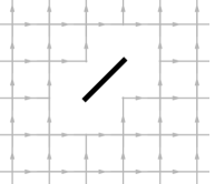
Figure 1: Example of a diagonal dimer. Its presence in the graph generates a new face of clockwise oddness $-1$: thus, as opposed to the case of the monomer defect Fisher and Stephenson (1963), the fermion representation of the diagonal dimer $\{{\bf x},{\bf x}+{\bf e}\}$ remains local and is $(-1)^{x_{1}+1}i\psi_{{\bf x}}\psi_{{\bf x}+{\bf e}}$.

III Interacting Fermions Picture

When $\lambda=0$ the dimer model is equivalent to a lattice fermion field without interaction. Namely

$$Z_{0}(\Lambda)=\int\!D\psi\;\exp\Big{\{}-\frac{1}{2}\sum_{{\bf x},{\bf y}}K_{{\bf x},{\bf y}}\psi_{\bf x}\psi_{\bf y}\Big{\}}$$ (6)

where: $\{\psi_{\bf x}:{\bf x}\in\Lambda\}$ are Grassmann variables and $D\psi$ indicates the integration w.r.t. all of them; $K_{{\bf x},{\bf y}}$ is the Kasteleyn matrix that can be chosen to be such that

$$\sum_{\bf y}K_{{\bf x},{\bf y}}\psi_{\bf y}=\sum_{\sigma=\pm 1}\sigma(\psi_{{\bf x}+\sigma{\bf e}_{0}}+i\psi_{{\bf x}+\sigma{\bf e}_{1}})$$

with ${\bf e}_{0}=(1,0)$ and ${\bf e}_{1}=(0,1)$. (6) is the partition function of a free Majorana fermion field, i.e. a Grassmann-valued Gaussian field with moment generator

$${\langle}e^{\sum_{\bf x}\psi_{\bf x}\eta_{\bf x}}{\rangle}_{0}=e^{-\frac{1}{2}\sum_{{\bf x},{\bf y}}S({\bf x}-{\bf y})\eta_{\bf x}\eta_{\bf y}}$$

where: the $\eta_{\bf x}$’s are other Grassmann variables; $S$, the covariance, is the inverse Kasteleyn matrix

$$S({\bf x})={\langle}\psi_{\bf x}\psi_{0}{\rangle}_{0}=\frac{1}{2}\int_{-\pi}^{\pi}\!\frac{dp_{0}}{2\pi}\int_{-\pi}^{\pi}\!\frac{dp_{1}}{2\pi}\;\frac{e^{ip_{0}x_{0}+ip_{1}x_{1}}}{i\sin p_{0}-\sin p_{1}}\;.$$

The Fourier transform of $S$ is singular at four Fermi momenta: ${\bf p}_{+,0}=(0,0)$, ${\bf p}_{+,1}=(\pi,\pi)$, ${\bf p}_{-,0}=(0,\pi)$ and ${\bf p}_{-,1}=(\pi,0)$. Therefore, in view of the scaling limit, it is convenient to decompose

$$\psi_{\bf x}=\sum_{\omega=\pm\atop s=0,1}i^{s}e^{i{\bf p}_{\omega,s}{\bf x}}\psi_{{\bf x},\omega,s}$$

where $\psi_{{\bf x},\omega,s}$ are four independent Majorana fields with large-$|{\bf x}|$ covariances

$${\langle}\psi_{{\bf x},\omega,s}\psi_{0,\omega,s}{\rangle}_{0}\; \sim\;\frac{1}{2}\int_{-\infty}^{\infty}\!\frac{dp_{0}}{2\pi}\int_{-\infty}^{\infty}\!\frac{dp_{1}}{2\pi}\;\frac{e^{ip_{0}x_{0}+ip_{1}x_{1}}}{ip_{0}-\omega p_{1}}$$

$$=\frac{1}{4\pi}\frac{1}{x_{0}+i\omega x_{1}}\;.$$ (7)

This decomposition already appeared in Fendley et al. (2002) for studying the free case, which is exactly solvable. Instead here we are preparing for the application to the interacting case and thus we also introduce Dirac spinors $\psi^{+}_{\bf x}=(\psi^{+}_{{\bf x},+},\psi^{+}_{{\bf x},-})$ and $\psi_{\bf x}=(\psi_{{\bf x},+},\psi_{{\bf x},-})^{T}$ for

$$\psi^{+}_{{\bf x},\omega}=\frac{\psi_{{\bf x},\omega,0}+i\psi_{{\bf x},\omega,1}}{\sqrt{2}}\quad\psi_{{\bf x},\omega}=\frac{\psi_{{\bf x},\omega,0}-i\psi_{{\bf x},\omega,1}}{\sqrt{2}}\;,$$ (8)

with translational invariant covariances

$${\langle}\psi_{{\bf x},\omega} \psi_{0,\omega^{\prime}}{\rangle}_{0}=0,\qquad{\langle}\psi^{+}_{{\bf x},\omega}\psi^{+}_{0,\omega^{\prime}}{\rangle}_{0}=0\;,$$

$${\langle}\psi^{+}_{{\bf x},\omega}\psi_{0,\omega^{\prime}}{\rangle}_{0}\;\sim\;\frac{\delta_{\omega,\omega^{\prime}}}{4\pi}\frac{1}{x_{0}+i\omega x_{1}}\;.$$ (9)

If we now let $\lambda\neq 0$, by power series expansion in $\lambda$ one can verify that (1) becomes

$$Z_{\lambda}(\Lambda)=\int\!D\psi\;\exp\Big{\{}-\frac{1}{2}\sum_{{\bf x},{\bf y}}K_{{\bf x},{\bf y}}\psi_{\bf x}\psi_{\bf y}+V(\lambda v,\psi)\Big{\}}\;,$$ (10)

where $V(\lambda v,\psi)$ is a sum of even monomials in the $\psi$’s of order bigger than two. It is not difficult to see that the dimer correlation in the l.h.s. of (II) becomes, in terms of Dirac fermions (8) and up to terms with faster decays

$${\langle}\psi_{0}\psi_{{\bf e}_{0}}\psi_{{\bf x}}\psi_{{\bf x}+{\bf e}_{0}}{\rangle}-{\langle}\psi_{0}\psi_{{\bf e}_{0}}{\rangle}{\langle}\psi_{{\bf x}}\psi_{{\bf x}+{\bf e}_{0}}{\rangle}$$

$$\sim 4(-1)^{x_{0}+x_{1}}\sum_{\omega}{\langle}\psi^{+}_{0,\omega}\psi_{0,\omega};\psi^{+}_{{\bf x},\omega}\psi_{{\bf x},\omega}{\rangle}^{T}$$

$$+4(-1)^{x_{0}}\sum_{\omega}{\langle}\psi_{0,\omega}^{+}\psi_{0,-\omega};\psi_{{\bf x},-\omega}^{+}\psi_{{\bf x},\omega}{\rangle}^{T}\;,$$ (11)

where the label $T$ indicates a truncated correlation. In the same way, the diagonal dimer correlation in the l.h.s. of (3) becomes

$$-(-1)^{x_{1}}\left[{\langle}\psi_{0}\psi_{{\bf e}}\psi_{{\bf x}}\psi_{{\bf x}+{\bf e}}{\rangle}-{\langle}\psi_{0}\psi_{{\bf e}}{\rangle}{\langle}\psi_{{\bf x}}\psi_{{\bf x}+{\bf e}}{\rangle}\right]$$

$$\sim-8\left[(-1)^{x_{0}+x_{1}}-1\right]{\langle}\psi^{+}_{0,+}\psi^{+}_{0,-};\psi_{{\bf x},-}\psi_{{\bf x},+}{\rangle}^{T}\;.$$ (12)

In the next section, by a Renormalization Group argument, we will explain why, in the evaluation of the large distance decay of the correlations, it is correct to replace the interacting fermion field (10) with the massless Thirring model. Assuming for the moment this crucial fact, we only need to borrow the exact solutions for the Thirring model correlations Johnson (1961); Klaiber (1964); Hagen (1967) (see also Falco (2012)):

$${\langle}\psi^{\dagger}_{\omega}(0)\psi_{\omega}(0);\psi^{\dagger}_{\omega}({\bf x})\psi_{\omega}({\bf x}){\rangle}^{T} =c\frac{x_{0}^{2}-x_{1}^{2}}{(x_{0}^{2}+x_{1}^{2})^{2}}$$

$${\langle}\psi^{\dagger}_{+}(0)\psi^{\dagger}_{-}(0);\psi_{-}({\bf x})\psi_{+}({\bf x}){\rangle}^{T} =\frac{c_{+}}{(x_{0}^{2}+x_{1}^{2})^{\kappa_{+}}}$$

$${\langle}\psi_{\omega}^{\dagger}(0)\psi_{-\omega}(0);\psi_{-\omega}^{\dagger}({\bf x})\psi_{\omega}({\bf x}){\rangle}^{T} =\frac{c_{-}}{(x_{0}^{2}+x_{1}^{2})^{\kappa_{-}}}$$ (13)

where the critical exponents $\kappa_{\pm}$ are

$$\kappa_{+}=\frac{1+\frac{\lambda_{T}}{4\pi}}{1-\frac{\lambda_{T}}{4\pi}}\qquad\kappa_{-}=\frac{1-\frac{\lambda_{T}}{4\pi}}{1+\frac{\lambda_{T}}{4\pi}}$$

and $\lambda_{T}$ is a parameter of the Thirring model: at first order $\lambda_{T}=-16\left[\hat{v}(\pi,\pi)-\hat{v}(0,\pi)\right]\lambda+O(\lambda^{2})$ (see next section). The derivation of (II), (3), (4) is complete.

IV RG Analysis

We follow Wilson’s RG scheme in the version due to Gallavotti Gallavotti (1985). Integrating out the large momentum scales, one obtains an effective interaction

$$\sum_{n}\sum_{\omega_{1},\ldots,\omega_{n}\atop s_{1},\ldots,s_{2n}}\frac{i^{s_{1}+\cdots s_{2n}}}{(2\pi)^{4n-1}}\int d{\bf k}_{1}\cdots d{\bf k}_{2n}\;{\widehat{\psi}}_{{\bf k}_{1},\omega_{1},s_{1}}\cdots{\widehat{\psi}}_{{\bf k}_{2n},\omega_{2n},s_{2n}}$$

$$\cdot\delta\Big{(}\sum_{j=1}^{2n}{\bf k}_{j}+\sum_{j=1}^{2n}{\bf p}_{\omega_{j},s_{j}}\Big{)}{\widehat{w}}_{2n}({\bf k}_{2}+{\bf p}_{\omega_{2},s_{2}},\ldots,{\bf k}_{2n}+{\bf p}_{\omega_{2n},s_{2n}})\;,$$

where ${\widehat{w}}_{2n}$’s are series of Feynman graphs. Some symmetries are of crucial importance. For $R(k_{0},k_{1})=(k_{1},-k_{0})$, $\vartheta(k_{0},k_{1})=(k_{1},k_{0})$ and $\tau(k_{0},k_{1})=(k_{0},k_{1}+\pi)$, we find

$${\widehat{w}}_{2m}(\tau{\bf k}_{2},\ldots,\tau{\bf k}_{2m})=(-i)^{m}{\widehat{w}}_{2m}(\vartheta{\bf k}_{2},\ldots,\vartheta{\bf k}_{2m})$$

$${\widehat{w}}_{2m}(R{\bf k}_{2},\ldots,R{\bf k}_{2m})=(-i)^{m}{\widehat{w}}_{2m}({\bf k}_{2},\ldots,{\bf k}_{2m})$$

$${\widehat{w}}_{2m}({\bf k}_{2},\ldots,{\bf k}_{2m})^{*}=i^{m}{\widehat{w}}_{2m}(\vartheta{\bf k}_{2},\ldots,\vartheta{\bf k}_{2m})\;.$$ (14)

From power counting, there are two possible local, marginal terms: a quartic term, that requires the renormalization of the coupling constant $\lambda$; a quadratic term, responsible for a field renormalization. By (IV) they are:

$$24{\widehat{w}}_{4}({\bf p}_{+,1},{\bf p}_{-,0},{\bf p}_{-,1})\sum_{{\bf x}}\psi_{{\bf x},+}^{+}\psi_{{\bf x},+}^{-}\psi_{{\bf x},-}^{+}\psi_{{\bf x},-}^{-}$$ (15)

and

$$2\left[-i\frac{\partial{\widehat{w}}_{2}}{\partial k_{0}}({\bf p}_{+,0})-\frac{\partial{\widehat{w}}_{2}}{\partial k_{1}}({\bf p}_{+,0})\right]\sum_{{\bf x},\omega}\psi_{{\bf x},\omega}^{+}\partial_{\omega}\psi_{{\bf x},\omega}^{-}\;,$$ (16)

where $\partial_{\omega}$ is the Fourier transform of $ik_{0}-\omega k_{1}$. Again by (IV), the prefactors in (15) and (16) are real. Instead, there are no local, relevant terms: the only possible one, a quadratic term without derivatives, i.e. a mass term, cannot be generated by conservation of total momentum. These facts imply that (10), with parameter $\lambda$, equals the massless Thirring model, with parameter $\lambda_{T}$, up to terms which are irrelevant and thus cannot modify (4) (although they do contribute to the relationship between $\lambda$ and $\lambda_{T}$ as series of Feynman graphs).

V Strong Interaction

In the opposite case of strong dimer interaction, i.e. $|\lambda|\gg 1$, the numerical findings of Alet et al. (2006) indicate the existence of four different “columnar” phases. Also this outcome can be theoretically explained: not by the IFP this time, but rather by the classical Peierls’ argument. However, as opposed to the weak interaction case, the outcome does depend on the choice of $v(d,d^{\prime})$: for definiteness, we discuss here the choice in Alet et al. (2006), which assigns an energy $-\lambda<0$ per each plaquette displaying one of the two dimer arrangements in Fig.2. Decorate a dimer configuration with wiggly lines as indicated in Fig.2: a plaquette is “good” if it contains 2 wiggly lines; otherwise, the plaquette is “bad”. Note that: a) dimer configurations on nearest neighbor good plaquettes must correspond to the same columnar ground state; b) the probability of a bad plaquettes occurrence is dumped, at least, by a factor $e^{-\frac{\lambda}{4}}$ per plaquette. Therefore one can apply the Peierls’ argument to the “contours” of bad plaquettes (see Heilmann and Lieb (1979); Fröhlich et al. (1980) or the review Biskup (2009)) and show that, for $\lambda$ positive and large, the number of different phases coincides with the number of ground states.

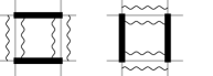
Figure 2: Draw four wiggly lines for each plaquette containing two facing dimers. An equivalent, but completely local way of evaluating the total energy of a dimer configuration is then by assigning an energy of $-\frac{\lambda}{4}$ per wiggly line.

VI Conclusion

In the case of weak short ranged interactions, we have showed that the IFP provides a detailed account of the numerical findings of Alet et al. (2006) –plus some new predictions. This method should also work, with possibly different outcomes, for triangular and hexagonal lattices; and for two or more interacting copies of dimer models. Besides, the IFP should be applicable to the Six-Vertex model, which is equivalent to dimers on a square lattice with a staggered interaction. Including the results on Ashkin-Teller, Eight-Vertex and XYZ quantum chain Benfatto et al. (2010) the IFP seems quite an effective way for dealing with two dimensional lattice critical models with central charge $c=1$. It might be possible that the IFP be applicable to $c<1$ models (for example via ideas in den Nijs (1983)).

In the case of strong aligning interactions, we have explained the numerical findings of Alet et al. (2006) by Peierls’ argument.

VII Acknowledgments

During the elaboration of the ideas and the the preparation of the work I benefited of several discussions with T. Spencer, M. Biskup and F. Bonetto.

References

- Kasteleyn (1963) P. Kasteleyn, J. Math. Phys. 4, 287 (1963).
- Lieb (1967) E. Lieb, J. Math. Phys. 8, 2339 (1967).
- Fisher and Stephenson (1963) M. Fisher and J. Stephenson, Phys. Rev. 132, 1411 (1963).
- Kenyon (1997) R. Kenyon, Ann. Inst. Henri Poincar Probab. Stat 33, 591 (1997).
- Dubédat (2011) J. Dubédat, arXiv:1110.2808 (2011).
- Fisher (1966) M. Fisher, J. Math. Phys. 7, 1776 (1966).
- Fan and Wu (1970) C. Fan and F. Wu, Phys. Rev. B 2, 723 (1970).
- Wu and Lin (1975) F. Wu and K. Lin, Phys. Rev. B 12, 419 (1975).
- Rokhsar and Kivelson (1988) D. Rokhsar and S. Kivelson, Phys. Rev. Lett. 61, 2376 (1988).
- Alet et al. (2005) F. Alet, J. Jacobsen, G. Misguich, V. Pasquier, F. Mila, and M. Troyer, Phys. Rev. Lett. 94, 235702 (2005).
- Alet et al. (2006) F. Alet, Y. Ikhlef, J. Jacobsen, G. Misguich, and V. Pasquier, Phys. Rev. E 74 (2006).
- Trousselet et al. (2007) F. Trousselet, P. Pujol, F. Alet, and D. Poilblanc, Phys. Rev. E 76, 041125 (2007).
- Otsuka (2009) H. Otsuka, Phys. Rev. E 80, 011140 (2009).
- Kadanoff (1978) L. Kadanoff, J. Phys. A 11, 1399 (1978).
- den Nijs (1983) M. den Nijs, Phys. Rev. B 27, 1674 (1983).
- Nienhuis (1984) B. Nienhuis, J. Stat. Phys. 34, 731 (1984).
- Jacobsen (2009) J. Jacobsen, in Polygons, Polyominoes and Polycubes, Lect. Notes Phys., Vol. 775 (2009) pp. 347–424.
- Fröhlich and Spencer (1981) J. Fröhlich and T. Spencer, Phys. Rev. Lett. 46, 1006 (1981).
- Solyom (1979) J. Solyom, Adv. in Phys. 28, 201 (1979).
- Giamarchi (2004) T. Giamarchi, Quantum physics in one dimension (Oxford University Press, USA, 2004).
- Spencer (2000) T. Spencer, J. Phys. A 279, 250 (2000), see also: H. Pinson and T. Spencer, Tech. Rep. (2000).
- Giuliani and Mastropietro (2004) A. Giuliani and V. Mastropietro, Phys. Rev. Lett. 93, 190603 (2004).
- Benfatto et al. (2010) G. Benfatto, P. Falco, and V. Mastropietro, Phys. Rev. Lett. 104, 75701 (2010).
- Fendley et al. (2002) P. Fendley, R. Moessner, and S. Sondhi, Phys. Rev. B 66, 214513 (2002).
- Yao and Kivelson (2012) H. Yao and S. Kivelson, Phys. Rev. Lett. 108, 247206 (2012).
- Kadanoff (1977) L. Kadanoff, Phys. Rev. Lett. 39, 903 (1977).
- Papanikolaou et al. (2007) S. Papanikolaou, E. Luijten, and E. Fradkin, Phys. Rev. B 76, 134514 (2007).
- Johnson (1961) K. Johnson, N. Cimento , 773 (1961).
- Klaiber (1964) B. Klaiber, Helv. Phys. Acta 37, 554 (1964).
- Hagen (1967) C. Hagen, N. Cimento B 51, 169 (1967).
- Falco (2012) P. Falco, arXiv:1208.6568 (2012).
- Gallavotti (1985) G. Gallavotti, Rev. Mod. Phys. 57, 471 (1985).
- Heilmann and Lieb (1979) O. J. Heilmann and E. H. Lieb, J. Stat. Phys. 20, 679 (1979).
- Fröhlich et al. (1980) J. Fröhlich, R. Israel, E. Lieb, and B. Simon, J. Stat. Phys. 22, 297 (1980).
- Biskup (2009) M. Biskup, Methods of Contemporary Mathematical Statistical Physics, Lect. Notes Math., Vol. 1970 (2009).