Ion-cyclotron Resonance with Streaming Bi-Maxwellian Distribution

Abstract

We investigate the effect of bulk velocity of the solar wind on the propagation characteristics of ion-cyclotron waves (ICWs). Our model is based on the kinetic theory. We solve the Vlasov equation for O VI ions and obtain the dispersion relation of ICWs. Refractive index of the medium for a streaming bi-Maxwellian velocity distribution proved to be higher than that of the bi-Maxwellian velocity distribution. The bulk velocity of the solar polar coronal holes’ plasma increases the value of the refractive index by a factor of 1.5 (3) when the residual contribution is included (neglected). The ratio of the refractive index of interplume lanes to the plume lanes at the coronal base is also higher than we found for the bi-Maxwellian velocity distribution, i.e. $k_{\rm interplume}/k_{\rm plume}=2.5$.

1 Introduction

The UVCS/SOHO observations of plasma properties in the polar coronal holes (PCH) revealed the existence of preferential ion heating with $T_{i}\gg T_{p}>T_{e}$ (Kohl et al., 1997a; 1998). Ion to proton kinetic temperature ratios are significantly higher than the ion to proton mass ratios, i.e. $T_{i}/T_{p}>m_{i}/m_{p}$ (Kohl et al. 1999). The UVCS measurements on PCH also provided clear signatures of temperature anisotropies, with the temperature perpendicular to the magnetic field being much larger than the temperature parallel to the field. The temperature anisotropy, for example, is found to be $T_{\perp}/T_{\parallel}\approx 10-100$ for O VI ions (Kohl et al., 1997b; 1998; Cranmer et al. 1999). These observations led to widespread interest in theoretical models of ion-cyclotron resonance (ICR), because this mechanism naturally produces preferential heating and temperature anisotropies (e.g. Dusenbery and Hollweg, 1981; Cranmer, 2001; Isenberg and Vasquez, 2009).

The ICR mechanism is a classical wave-particle interaction between the left-hand polarized ion-cyclotron/Alfv$\acute{\rm e}$n waves and the positive ions gyrating around the background magnetic field lines. Resonance occurs when the Doppler-shifted wave frequency and the ion cyclotron frequency are equal. When the resonance condition is met, the electric field oscillations of the wave are no longer “felt” by the ion. Therefore, the ion sees a constant electric field and can efficiently absorb energy from the wave depending on the relative phase between its own velocity vector and the electric field vector of the wave. The resulting effect of this process is to increase the perpendicular velocity of the ion (Isenberg and Vasquez, 2009; Cranmer 2009). Ions with higher perpendicular energy diffuse into wider Larmor orbits. The preferential perpendicular heating indicated by UVCS measurements naturally leads to a preferential acceleration since the ions having greater perpendicular velocities experience a higher mirror force, $F_{\rm mf}(R)=-\mu\nabla B=-[(1/2)m_{\rm i}v^{2}_{\bot}/B(R)]\nabla B$, in the radially decreasing magnetic field of the coronal hole.

In a series of papers by Hollweg (1999a, b, c) the authors investigated the resonant interactions with ion-cyclotron waves in coronal holes in detail. Besides, Hollweg and Markovskii (2002) offered a physical discussion of how the cyclotron resonances behave when the waves propagate obliquely to the magnetic field. Vocks and Marsch (2002) described a kinetic model which is based on wave-particle interactions. Their model successfully explains the preferential heating of heavy ions and the temperature anisotropies. Cranmer (2000) investigated the dissipation of ion-cyclotron resonant waves by taking more than 2000 ion species into account and showed the effective damping ability of the minor ions.

There are also a number of theoretical models which are based on fluid or magnetohydrodynamic approaches to the coronal heating and the solar wind acceleration (e.g. Tu and Marsch, 1997; Suzuki and Inutsuka, 2006; Matsumoto and Suzuki, 2012). The suggested fluid models can successfully produce the required energy flux density to heat the coronal holes without resonant interactions. However, the kinetic approach has an advantage of distinguishing the plasma particles in a more definitive way in accordance with the collisionless nature of PCH (Cranmer, 2009). A kinetic description is required in order to account fully for the observed microscopic details of the solar wind plasma (Marsch, 1991). Since the ICR process successfully explains the details revealed by the observations, i.e. the presence of temperature anisotropy of minor ion species and preferential heating, it has been proposed as the most favourable heating mechanism of the solar corona.

Over the last few years, there has been an enormous increase in the number of observations on ubiquitous waves in the solar corona. Tomczyk et al. (2007) detected MHD waves by using Coronal Multi-Channel Polarimeter (CoMP). Their estimate of the energy carried by the spatially resolved waves indicates that the waves are too weak to heat the solar corona; however they also proposed that the unresolved MHD waves can carry enough energy to heat the corona. Recently, McIntosh et al. (2011) measured the amplitudes, periods and phase speeds of outward-propagating Alfvénic motions in the transition region and the corona. They reported that the observed waves are energetic enough to accelerate the fast solar wind and heat the quiet corona. Besides, the observations of Hahn et al. (2012) provide a new evidence of wave damping at unexpectedly low heights in a polar coronal hole (PCH). They estimate that the dissipated energy may account for a large fraction (up to about 70%) of that required to heat the coronal hole and accelerate the fast solar wind.

In Doğan & Pekünlü (2012, hereafter Paper I) we studied the effect of the plume and interplume lanes (PIPL) of PCHs on the interaction between the O VI ions and the ion-cyclotron waves (ICWs). In Paper I as well as in the present one, the gradients of number density and temperature along and perpendicular to the magnetic field lines were considered. It was shown in Paper I that the resonance process in the interplume lanes is much more effective than in the plumes. Nevertheless, we should mention that more efficient dissipation may not necessarily lead to a higher wind flow. It is discussed by some authors that a stronger heating rate is required to produce the denser wind flows in the plume regions where the bulk speed is observed to be slower (see e.g. Wang, 1994; Pinto et al. 2009).

The present investigation is the extension of Paper I wherein we assumed that O VI ions have a bi-Maxwellian velocity distribution function in PCHs. In this study, we assume that the streaming bi-Maxwellian velocity distribution function for O VI ions would be physically more realistic than that of bi-Maxwellian, since the former will take into consideration the bulk velocity of the solar wind. The paper is structured as follows: In section 2, we briefly summarize the plasma properties of the PCHs and obtain the dispersion relation of the ICWs solving the Vlasov equation for O VI ions. We also compare the new results with those found in Paper I. We present our conclusions in Section 3.

2 Model

2.1 Plasma properties of PCH

Properties of the PCH plasma were explained in Paper I in greater detail (see section 2 of Paper I and references therein). Here, we only summarize the radial dependences of effective temperature, number density, the PCH magnetic field and the bulk velocity of O VI ions, respectively. By using the empirical model of Cranmer et al. (1999), Banerjee et al. (2000) derived a best-fit function for the O VI line width which is valid in the range 1.5-3.5 $\rm R_{\odot}$. When we convert their Eq. (3) into the effective temperature, we get the radial dependence of $T_{\rm eff}$ as below:

$$T_{\rm{eff}}(R)=4.02\times 10^{7}R^{2}+1.25\times 10^{7}R-9.76\times 10^{7}\,\,\,\rm K.$$ (1)

where R is the dimensionless radial distance, i.e., R=r/$\rm R_{\odot}$. By using the polarized white light and line ratio measurements in northern PCH, Esser et al. (1999) derived an analytical expression for the electron number density:

$$N_{\rm{e}}(R)=2.494\times 10^{6}R^{-3.76}+1.034\times 10^{7}R^{-9.64}+3.711\times 10^{8}R^{-16.86}\,\,\,\rm cm^{-3}.$$ (2)

Radial dependence of PCH magnetic field is given by Hollweg (1999a) as below:

$$B=1.5(f_{\rm max}-1)R^{-3.5}+1.5R^{-2}\,\,\rm Gauss$$ (3)

where $f_{\rm max}=9$. The radial dependence of O VI cyclotron frequency ($\omega_{\rm c}=q_{\rm i}B/m_{\rm i}c$) will be calculated by using Eq. (3).

Verdini et al. (2012) present a solar wind speed profile in the radial direction. By using their Fig. 1, we express the radial dependence of the wind speed with the equation given below,

$$\emph{u}=5R^{3}-45R^{2}+140R+150\,\,\rm kms^{-1}.$$ (4)

This relation is valid in the distance range 1.5-3.5 R. We should mention that the solar wind speed profile strongly depends on the magnetic field profile assumed in the wind model of Verdini et al. (2012). The magnetic field profiles of Verdini et al. (2012) and Hollweg (1999a) overlap quite a lot with appropriate values of free parameters. Nevertheless, our calculation may include an imprecision resulting from the possible inconsistency of two profiles. An interested reader may refer to Pinto et al. (2009) and Grappin et al. (2010) for alternative profiles.

We also consider the PIPL structure of PCH, the physical parameters of which display gradients along and perpendicular direction to the external magnetic field. Wilhelm et al. (1998) report that the effective temperature of O VI ions in the interplume lanes are about 30% higher than that of plumes. By using this observational result Devlen $\&$ Pekünlü (2010) formulate the temperature structure of PCH in two dimensions as below:

$$T_{\rm{eff}}(R,x)=T_{\rm{eff}}(R)+0.3T_{\rm{eff}}(R)\sin^{2}(\frac{2\pi}{\lambda}x)$$ (5)

where x is the direction perpendicular to R and $\lambda$ is the expansion rate of the widths of PIPL in PCH in arcseconds, i.e., $\lambda=92^{\prime\prime}.16R$. The factor 0.3 comes from the temperature difference between the plume and interplume lane. The number densities of electrons in plumes appear to be 10% higher than that of interplume lanes (Kohl et al., 1997a). When we consider this difference, we can express the number density of O VI ions in (R,x) plane as below:

$$N_{\rm{i}}(R,x)=fN_{\rm{p}}^{\rm{PL}}(R)[1-0.1\sin^{2}(2\pi x/\lambda)]\,\,\,\rm cm^{-3}$$ (6)

where f is the mean value of O VI number density ($1.52\times 10^{-6}N_{\rm p}$) as given by Cranmer et al. (2008). The factor 0.1 comes from the difference of the number densities between plumes and interplumes. We will use these observational results to solve the Vlasov equation in the next subsection.

2.2 Solution of the Vlasov Equation

It is appropriate to use Vlasov equation to describe the collisionless plasma like coronal holes in time intervals shorter than the interspecies collision time. In this method, the first-order perturbations to the velocity distribution function is calculated in coordinates that follow the unperturbed trajectory of the particles. Knowledge of the perturbed velocity in terms of the first-order electric field allows us to calculate the current density and the dielectric tensor. Substitution of dielectric tensor into wave equation gives the dispersion relation for the ICWs (Stix, 1992). We follow the same procedure as we did in Paper I and adopt the space time variation of the perturbed quantities as $\exp[i(\emph{{k}}\cdot\emph{{r}}-\omega t)]$. Wave equation is given (e.g. Stix, 1962, 1992) as below,

$$\textbf{k}\times\left(\textbf{k}\times\textbf{E}\right)+\frac{\omega^{2}}{c^{2}}\kappa\cdot\textbf{E}=0$$ (7)

where $\kappa$ is the dielectric tensor and conventionally is derived from the Vlasov equation. We again assume that both the Lorentz force, $q[\textbf{E}+\frac{1}{c}(\textbf{v}\times\textbf{B}_{0})]$ and the pressure gradient force, $-\nabla p$ act upon O VI ions, where symbols throughout this paper are the same as in Paper I and have their usual meanings. With these assumptions, the quasi-linearized Vlasov equation is written as,

$$\begin{array}[]{l}\frac{{\it d}\,{\it f}_{1}}{{\it d}\,{\it t}}=\frac{\partial\,{\it f}_{1}}{\partial\,{\it t}}+\textbf{v}\cdot\frac{\partial\,{\it f}_{1}}{\partial\,\textbf{R}}+\frac{{\it q}_{\rm i}}{{\it m}_{\rm i}}\left(\textbf{E}_{1}+\frac{1}{c}(\textbf{v}\times\textbf{B}_{0})\right)\cdot\frac{\partial\,{\it f}_{1}}{\partial\,\textbf{v}}=\bigg{[}-\frac{{\it q}_{\rm i}}{{\it m}_{\rm i}}\left(\textbf{E}_{1}+\frac{1}{c}(\textbf{v}\times\textbf{B}_{1})\right)\\ \\ +\frac{{\it k}_{\rm B}}{n_{0}m_{\rm i}}\left(T_{\rm eff}^{\rm\xi}\frac{\partial n_{\rm 0}}{\partial\textbf{R}}+T_{\rm eff}^{\rm\xi}\frac{\partial n_{0}}{\partial\textbf{x}}+n_{0}\frac{\partial T_{\rm eff}^{\rm\xi}}{\partial\textbf{R}}+n_{0}\frac{\partial T_{\rm eff}^{\rm\xi}}{\partial\textbf{x}}\right)\bigg{]}\cdot\frac{\partial\,{\it f}_{0}}{\partial\textbf{v}}.\end{array}$$ (8)

where $f_{0}$ and $f_{1}$ are the unperturbed and perturbed parts of the velocity distribution function and $\textbf{E}_{1}$ and $\textbf{B}_{1}$ are the wave electric and magnetic fields, respectively. The time derivative is taken along the unperturbed trajectories in phase - space of O VI ions. Schmidt (1979) gives Left Circularly Polarized (LCP) wave interacting with the perturbed velocity function of ions as,

$$\begin{array}[]{l}{f_{\rm L}=}{-\frac{q_{\rm i}}{m_{\rm i}}\left[\left(1-\frac{v_{\parallel}k}{\omega}\right)\frac{\partial\,f_{0}}{\partial\,v_{\bot}}+\frac{k\,v_{\bot}}{\omega}\frac{\partial\,f_{0}}{\partial\,v_{\parallel}}\right]E_{\rm x}\exp\,\left(i\theta_{0}\right)\frac{1-\exp\phi}{i(k\,v_{\parallel}-\omega+\omega_{c})}+\nabla p_{1}}\end{array}$$ (9)

where $\nabla p_{1}$ is

$$\nabla p_{1}=\frac{{\it k}_{\rm B}}{n_{0}m_{\rm i}}\left(T_{\rm eff}^{\xi}\frac{\partial n_{0}}{\partial\textbf{R}}+T_{\rm eff}^{\xi}\frac{\partial n_{0}}{\partial\textbf{x}}+n_{0}\frac{\partial T_{\rm eff}^{\xi}}{\partial\textbf{R}}+n_{0}\frac{\partial T_{\rm eff}^{\xi}}{\partial\textbf{x}}\right)$$ (10)

$f_{1}$ produces a current, x and y components of which are given in Paper I. Using these currents one can derive the plasma dielectric tensor for LCP wave as:

$$\begin{array}[]{l}{\kappa_{L}=1+4\pi\frac{J_{\rm x}/E_{\rm x}}{i\,\omega\ }=}{1-\frac{4\pi^{2}\,q_{\rm i}^{2}}{im_{\rm i}\ \omega^{2}}\int_{-\infty}^{+\infty}d\,v_{\parallel}\int_{0}^{\infty}\frac{\left(\omega-k\,v_{\parallel}\right)\,\left(\partial\,f_{0}/\partial\,v_{\bot}\right)+k\,v_{\bot}\left(\partial\,f_{0}/\partial\,v_{\parallel}\right)}{k\,v_{\parallel}-\omega+\omega_{c}}(1-\exp\phi)v_{\bot}^{2}\,d\,v_{\bot}}\\ \\ +{\frac{4\pi^{2}q_{i}}{\omega E_{\rm x}}(t-t_{0})\int_{0}^{\infty}\nabla p_{1}v_{\bot}^{2}\,dv_{\bot}\,dv_{\parallel}}.\end{array}$$ (11)

We will obtain the dispersion relation for LCP wave by substituting Eq. (11) into $\kappa_{L}=n^{2}=c^{2}k^{2}/\omega^{2}$ where n is the refractive index of the medium for ICWs.

Observations revealed that PCHs’ collisionless and streaming plasma displays temperature anisotropies. Bearing these observational facts in mind, we proceed our investigation with a streaming bi-Maxwellian velocity distribution function for O VI ions,

$$f_{0}=n_{\rm i}\,\alpha_{\bot}^{2}\alpha_{\parallel}\,\pi^{-3/2}\exp\left[-\left(\alpha_{\bot}^{2}v_{\bot}^{2}+\alpha_{\parallel}^{2}(v_{\parallel}-u)^{2}\right)\right]$$ (12)

where u represents the overall bulk velocity of the PCH plasma and $\alpha_{\bot}=(2k_{\rm B}T_{\bot}/m_{i})^{-1/2}$ and $\alpha_{\parallel}=(2k_{\rm B}T_{\parallel}/m_{i})^{-1/2}$ are the inverse of the most probable speeds in the perpendicular and parallel direction to the external magnetic field, respectively. The velocity derivatives of $f_{0}$ which will be substituted in Eq. (11) are obtained from Eq. (12) and finally the contribution of the principle integral to the dispersion relation of LCP wave is found as below,

$$\begin{array}[]{l}{k^{2}\,\left(c^{2}-\frac{\omega^{2}}{k^{2}}\right)-\frac{i\omega_{p}^{2}\,\omega}{\left(\omega-\omega_{c}\right)}-\frac{i\omega_{p}^{2}\,ku}{\,\left(\omega-\omega_{c}\right)}\left[\frac{T_{\bot}}{T_{//}}\left(\frac{ku}{(\omega-\omega_{c})}+2\right)-\frac{\omega}{(\omega-\omega_{c})}-1\right]}\\ {}\\ {-\frac{i\omega_{p}^{2}k^{2}\left(1+2\alpha_{//}^{2}u^{2}\right)}{2\alpha_{//}^{2}\left(\omega-\omega_{c}\right)^{2}}\left(\frac{\omega\,}{\left(\omega-\omega_{c}\right)}-\frac{T_{\bot}}{T_{//}}+1\right)+\frac{\pi^{2}\omega{\it q}_{i}\,L}{{\it E}_{\rm x}v_{A}}\nabla p_{1}^{\rm r}=0}\end{array}$$ (13)

where $\omega_{p}=(4\pi n_{OVI}q_{i}^{2}/m_{i})^{1/2}$ is the plasma frequency for the O VI ions and $\nabla p_{1}^{r}$ is the term designating rather lengthy pressure gradient in its reduced form:

$$\nabla p_{1}^{\rm r}=\frac{{\it k}_{\rm B}}{m_{\rm i}}\left[{\left(T_{\rm eff}^{\xi}\frac{\partial n_{0}}{\partial R}+n_{0}\frac{\partial T_{\rm eff}^{\xi}}{\partial R}\right)\left(\frac{T_{\bot}}{T_{\parallel}}\right)^{1/2}}+2\left(T_{\rm eff}^{\xi}\frac{\partial n_{0}}{\partial x}+n_{0}\frac{\partial T_{\rm eff}^{\xi}}{\partial x}\right)\right].$$ (14)

The residual contribution is found as,

$$\Re=\frac{2\sqrt{\pi}\omega_{p}^{2}}{k}\,\alpha_{//}\left[\omega_{c}+(\omega-\omega_{c}-uk)\frac{T_{\bot}}{T_{//}}\right]\exp\left[-\alpha_{//}^{2}\left(\frac{\omega-\omega_{c}}{k}-u\right)^{2}\right].$$ (15)

The dispersion relation is the combination of the principle and the residual contribution given in Eqs (13) and (15) respectively:

$$\begin{array}[]{l}{k^{2}\,\left(c^{2}-\frac{\omega^{2}}{k^{2}}\right)-\frac{i\omega_{p}^{2}\,}{\left(\omega-\omega_{c}\right)}\left[\omega+ku\frac{T_{\bot}}{T_{//}}+ku\Psi+\frac{k^{2}\left(1+2\alpha_{//}^{2}u^{2}\right)}{2\alpha_{//}^{2}\left(\omega-\omega_{c}\right)}\Pi\right]}\\ {}\\ +\frac{\pi^{2}\omega{\it q}_{i}\,L}{{\it E}_{\rm x}v_{A}}\nabla p_{1}^{\rm r}{-\frac{2\sqrt{\pi}\omega_{p}^{2}}{k}\,\alpha_{//}\Phi\exp\left[-\alpha_{//}^{2}\left(\frac{\omega-\omega_{c}}{k}-u\right)^{2}\right]=0}\end{array}$$ (16)

where $\Psi$, $\Pi$ and $\Phi$ are

$$\begin{array}[]{l}{\Psi=\left[\frac{2T_{\bot}}{T_{//}}-\frac{\omega}{(\omega-\omega_{c})}-1\right]}\\ \\ {\Pi=\left[\frac{\omega\,}{\left(\omega-\omega_{c}\right)}-\frac{T_{\bot}}{T_{//}}+1\right]}\\ \\ {\Phi=\left[\omega_{c}(\omega-\omega_{c})^{2}+\frac{T_{\bot}}{T_{//}}\left(\omega^{3}-3\omega^{2}\omega_{c}+3\omega\omega_{c}^{2}-\omega_{c}^{3}\right)\right]}.\end{array}$$ (17)

If we expand the exponential factor appearing in the last term of the Eq. (16) into Taylor series, we get the Dispersion Relation I (DR I) as below,

$$\begin{array}[]{l}{k^{5}\left[c^{2}-\frac{i\omega_{p}^{2}u^{2}}{(\omega-\omega_{c})^{2}}\frac{T_{\bot}}{T_{\parallel}}-\frac{i\omega_{p}^{2}\left(1+2\alpha_{//}^{2}u^{2}\right)}{2\alpha_{//}^{2}\left(\omega-\omega_{c}\right)^{2}}\Pi\right]-k^{4}\frac{{\it i}\omega_{p}^{2}\,u}{\,\left(\omega-\omega_{c}\right)}\Psi}\\ {}\\ {-k^{3}\left[\omega^{2}+\frac{{\it i}\omega_{p}^{2}\,\omega}{\left(\omega-\omega_{c}\right)}-\frac{\pi^{2}\omega{\it q}_{{\it i}}\,L}{{\it E}_{{\rm x}}v_{A}}\nabla p_{1}^{\rm r}+2\sqrt{\pi}\omega_{p}^{2}\,\alpha_{//}^{3}u\frac{T_{\bot}}{T_{\parallel}}\right]}\\ {}\\ {-2\sqrt{\pi}\omega_{p}^{2}\,\alpha_{//}k^{2}\left[\omega_{c}+\omega_{c}\alpha_{//}^{2}u^{2}+\left(\omega-\omega_{c}\right)\frac{T_{\bot}}{T_{\parallel}}\left(1-3\alpha_{//}^{2}u^{2}\right)\right]}\\ {}\\ {+{\it 2}\sqrt{\pi}\omega_{p}^{2}\,\alpha_{{}_{//}}{\it k}\left[3u\alpha_{//}^{2}\frac{T_{\bot}}{T_{\parallel}}\left(\omega-\omega_{c}\right)-2u\omega_{c}\alpha_{//}^{2}\left(\omega+\omega_{c}\right)\right]}{{\it+2}\sqrt{\pi}\omega_{p}^{2}\,\alpha_{{}_{//}}^{3}{\Phi}=0}\end{array}$$ (18)

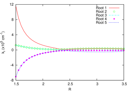
Figure 1: All five roots of the fifth order DRI given by Eq. (18). The graph is for ICWs with a frequency 2500 $\rm rads^{-1}$.

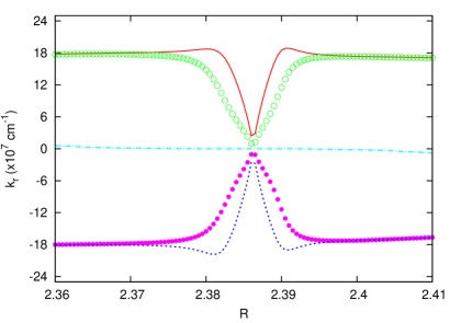
Figure 2: Fig. 1 is zoomed in the reflection region. Root 3 shows reflection at R=2.385. The same symbols are used with Fig. 1.

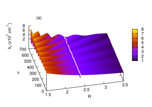
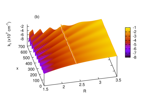
Figure 3: Two roots of DR II. (a) First root of DRII. This root represents the backward propagating mode, (b) Second root of DR II. This root represents the forward propagating mode. Both roots reveal resonance at R=2.38. The higher values of $k_{r}$ in interplume lanes point to more effective resonance process. The graphs are for ICWs with a frequency 2500 $\rm rads^{-1}$.

The real parts of all five roots of DR I (Eq. 18) are presented in Fig. 1 in the radial distance range 1.5 R-3.5 R. According to Shevchenko’s criterion (2007), that is, $Imk^{2}=2k_{r}k_{i}\gtrless 0$ where the upper (lower) sign is for the backward (forward) wave, roots 1, 2, 3 and 5 represent the backward propagating modes and root 4 is the forward propagating mode. It is shown in Fig. 1 that all roots with a frequency of 2500 rads^-1 merge at about 2.38 R similar to the Fig. 2 of Paper I. This location is the site where ion cyclotron resonance and cut-offs take place in a small range of distance. Here we should remind the reader that the field function of the wave is assumed of the form, $exp[i(\textbf{k}\cdot\textbf{r}-\omega t)]=exp[i(\textbf{k}_{r}\cdot\textbf{r}-\omega t)]exp(-\textbf{k}_{i}\cdot\textbf{r})$. Therefore, the situation where $k_{r}\rightarrow\infty$ corresponds to the refractive index going to infinity and implies a resonance. The situation where $k_{r}=0$ implies a cutoff and corresponds to a wave reflection. If the solution of the dispersion relation yields $k_{i}>0$ then the wave damps in the r-direction. Differing from our previous results, the real part of the wavenumber of the third mode becomes zero, corresponding to a reflection at R=2.385. In going through cutoff, a transition is made from a region of propagation to a region of evanescence. This result is consistent with the positive values of the imaginary part of this root after reflection. The amplitude of the mode shows a decay through the radial distance indicating that the medium is not an idealized reflector. No matter how small the decrease in wave amplitude is, the dissipated wave energy is transferred to the O VI ions (Melrose & McPhedron, 1991).

The other difference from previous results is the value of the wavenumbers. The wavenumbers are found to be, on average, 1.5 times higher than those found in Paper I. The inclusion of the bulk velocity of the PCHs’ plasma increases the value of the refractive index of the medium. In other words, the phase velocity of the ICWs are found to be slower when the bulk velocity is taken into consideration.

The reflection region where the refractive index is equal to zero for root 3 is zoomed in Fig. 2. This wave attenuates spatially after reflection. Fig. 2 also shows the modulational behaviour of the root 1, 2, 4 and 5 in the same reflection region. These modes approach zero at R=2.385, however they do not show reflection. We should also mention that the inclusion of the gradients in the x-direction through the PIPL structure does not alter the solution of DR I. The refractive index is found to be a function of radial distance (R) only. We will show the effect of PIPL structure on the refractive index in the solution of DR II.

The highest value of the residual contribution is found to be $10^{-12}$ and this value is negligibly small compared to the values of the rest of the terms which range between $10^{6}$ - $10^{13}$ in the Eq. (16). If we neglect the residual contribution in the dispersion relation given by Eq. (16) then Eq. (18) is reduced to DR II given below:

$${\it k}^{2}\left[{\it c}^{2}-\frac{\it i\omega_{p}^{2}u^{2}}{(\omega-\omega_{c})^{2}}\frac{{\it T}_{\bot}}{{\it T}_{{\it\parallel}}}-\frac{i\omega_{p}^{2}\left(1+2\alpha_{//}^{2}u^{2}\right)}{2\alpha_{//}^{2}\left(\omega-\omega_{c}\right)^{2}}\Pi\right]-\frac{{\it i}\omega_{p}^{2}\,{\it ku}}{\,\left(\omega-\omega_{c}\right)}\Psi-\frac{{\it i}\omega_{p}^{2}\,\omega}{\left(\omega-\omega_{c}\right)}-\omega^{2}+\frac{\pi^{2}\omega{\it q}_{{\rm i}}\,L}{{\it E}_{{\rm x}}v_{A}}\nabla p_{1}^{\rm r}=0$$ (19)

The graphical solution of DR II is given in Fig. 3. As we mentioned above, this solution reveals an infinity in the refractive index indicating that a resonance occurs at R =2.38. The refractive index is, on average, 3 times higher than those found in Paper I. Including the bulk velocity of the solar wind clearly increases the value of the refractive index. This result again implies that the phase velocity of the ICWs becomes slower when the bulk velocity is taken into consideration. Besides, the effect of the PIPL structure is clearly seen in Figs. 3a-b. The real part of the wavenumbers reveal a change both in R and x-direction. The crests correspond to the interplume lanes and the troughs to the plume lanes. The refractive index in the interplume lanes are found to be about 2.5 times higher than the ones in the plumes at the coronal base. We may anticipate that the refractive index of the interplume lanes is readily going to infinity indicating that the resonance process in the interplume lanes is more effective than in the plumes.

3 Conclusions

In this paper, the effect of the PIPL structure of PCH is re-discussed with the assumption of streaming bi-Maxwellian velocity distribution which is expected to be more realistic for the PCH plasma. The wavenumbers of ICWs for a streaming bi-Maxwellian velocity distribution is found to be 1.5-3 times higher than that of the bi-Maxwellian velocity distribution. Since the wave frequency we assumed, i.e. 2500 $\rm rads^{-1}$, is the same in both investigation, the higher wavenumber implies that the phase velocity of the ICWs becomes slower when the bulk velocity is taken into consideration. Wave spectrum in PCHs determines the net acceleration to be acquired by the O VI ions having a streaming bi-Maxwellian velocity distribution.

The refractive index is 2.5 times higher in interplume lanes than the one in plume lanes. This ratio is slightly higher than we found for the bi-Maxwellian distribution assumption. Higher refractive index may imply that the resonance process is more effective in interplume regions. However, it is yet to be discussed whether a stronger heating is needed in order to produce faster flows of the interplume lanes (see Pinto et al. 2009). If more efficient resonance process means a higher wind speed, than our result is consistent with the observations which reveal that the source of the fast solar wind is interplume lanes.

Let us suppose that an O VI ion resonates with a wave of a certain frequency, gains energy and escapes from the potential well of the wave. If there is a wave with a higher frequency in the surrounding, O VI ions come into resonance with it too and acquire more energy. In order stochastic acceleration to come about there should be a wide band of waves in PCHs. McIntosh et al. (2011) measured the phase speeds, amplitudes and periods of the transverse waves both in the quiet corona and PCHs. As to whether they also determined the frequency band of the waves is unknown to the authors of the present investigation.

In ICR process energy of the waves are transferred to the perpendicular degree of freedom of the O VI ions in their helical trajectories around magnetic field lines. Those particles the velocity of which are equal to the phase velocity ($v=\omega/k$) are readily trapped in the potential wells of the waves. Particles with velocities slightly higher than the phase velocity of the wave attempt to escape from the potential well of the wave, fail in this attempt fall back and set in a oscillatory motion in the potential well. These kind of particles, because of their initial velocity were higher than the phase velocity of the wave, becomes slower and on the average give up part of their energy to the wave and cause the amplitude of the wave grow. On the other hand, the O VI ions with velocities slower than the phase velocity of the wave acquire acceleration, gain energy at the expense of the wave energy.

If the streaming bi-Maxwellian velocity distribution function has a negative slope then the number of particles causing the wave damping is greater than the number of particles causing the wave growth. In this case, the net effect of the ICR process is the transfer of energy from ICWs to O VI ions.

References

- Banerjee et al. (2000) Banerjee, D., Teriaca, L., Doyle, J. G. et al. 2000, SoPh, 194, 43
- Cranmer et al. (1999) Cranmer, S. R., Field, G. B., & Kohl, J. L. 1999, ApJ, 518, 937
- Cranmer (2000) Cranmer, S. R. 2000, ApJ, 532, 1197
- Cranmer (2001) Cranmer, S. R. 2001, JGR, 106, 24937
- Cranmer et al. (2008) Cranmer, S. R., Panasyuk, A. V., & Kohl, J. L. 2008, ApJ, 678, 1480
- Cranmer (2009) Cranmer, S. R. 2009, Living Reviews in Solar Physics, 6, 3
- Devlen & Pekünlü (2010) Devlen, E., & Pekünlü, E. R. 2010, AN, 331, 716
- Doğan & Pekünlü (2012) Doğan, S., & Pekünlü, E. R. 2012, NewA, 17, 316
- Dusenbery & Hollweg (1981) Dusenbery, P. B., & Hollweg, J. V. 1981, JGR, 86, 153
- Grappin et al. (2010) Grappin, R., Leorat, J., Leygnac, S.,& Pinto, R. 2010, AIPC, 1216, 24
- Esser et al. (1999) Esser, R., Fineschi, S., Dobrzycka, D. et al. 1999, ApJ, 510, L63
- Hahn et al. (2012) Hahn, M., Landi, E., & Savin, D. W. 2012, ApJ, 753, 36
- Isenberg & Vasquez (2009) Isenberg, P. A., & Vasquez, B. J. 2009, ApJ, 696, 591
- Hollweg (1999) Hollweg, J. V. 1999a, JGR, 104, 505
- Hollweg (1999) Hollweg, J. V. 1999b, JGR, 104, 24781
- Hollweg (1999) Hollweg, J. V. 1999c, JGR, 104, 24793
- Hollweg & Markovskii (2002) Hollweg, J. V., & Markovskii, S. A. 2002, JGR, 107, 1080
- Kohl et al. (1997) Kohl, J. H., Noci, G., Antonucci, E., et al. 1997a, Advances in Space Research, 20, 3
- Kohl et al. (1997) Kohl, J. L., Noci, G., Antonucci, E., et al. 1997b, SoPh, 175, 613
- Kohl et al. (1998) Kohl, J. L., Noci, G., Antonucci, E., et al. 1998, ApJ, 501, L127
- Kohl et al. (1999) Kohl, J. L., Esser, R., Cranmer, S. R., et al. 1999, ApJ, 510, L59
- Marsch (1991) Marsch, E. 1991, Physics of the Inner Heliosphere 21, Springer, Newyork
- Matsumoto & Suzuki (2012) Matsumoto, T., & Suzuki, T. K. 2012, ApJ, 749, 8
- Melrose & McPhedran (1991) Melrose, D. B., & McPhedran, R. C. 1991, Electromagnetic Processes in Dispersive Media, Cambridge, UK: Cambridge University Press
- McIntosh et al. (2011) McIntosh, S. W., de Pontieu, B., Carlsson, M., Hansteen, V., Boerner, P., & Goossens, M. 2011, Nature, 475, 477
- Pinto et al. (2009) Pinto, R., Grappin, R., Wang, Y.-M., & Leorat, J. 2009, A&A, 497, 537
- Schmidt et al. (1979) Schmidt, G., 1979, Physics of High Temperature Plasmas, 2nd. ed., Academic Press, New York
- Shevchenko (2007) Shevchenko, V.V. 2007, Physics - Uspekhi 50 (3) 287-292
- Stix (1962) Stix, T.H. 1962, The Theory of Plasma Waves, McGraw - Hill Book Co., New York
- Stix (1992) Stix, T. H. 1992, Waves in Plasmas, Springer
- Suzuki & Inutsuka (2006) Suzuki, T. K., & Inutsuka, S.-i. 2006, JGR, 111, 6101
- Tomczyk et al. (2007) Tomczyk, S., McIntosh, S. W., Keil, S. L. et al. 2007, Science, 317, 1192
- Tu & Marsch (1997) Tu, C.-Y., & Marsch, E. 1997, SoPh, 171, 363
- Wang (1994) Wang, Y.-M. 1994, ApJ, 435, L153
- Wilhelm et al. (1998) Wilhelm, K., Marsch, E., Dwivedi, B. N. et al. 1998, ApJ, 500, 1023
- Verdini et al. (2012) Verdini, A., Grappin, R., Pinto, R., & Velli, M. 2012, ApJL, 750, L33
- Vocks & Marsch (2002) Vocks, C., & Marsch, E. 2002, ApJ, 568, 1030